



Abstract
Cross-level interaction effects lay at the heart of multilevel contingency and interactionism theories. Also, practitioners are particularly interested in such effects because they provide information on the contextual conditions and processes under which interventions focused on individuals (e.g., selection, leadership training, performance appraisal, and management) result in more or less positive outcomes. We derive a new intraclass correlation, ρβ, to assess the degree of lower-level outcome variance that is attributed to higher-level differences in slope coefficients. We provide analytical and empirical evidence that ρβ is an index of variance that differs from the traditional intraclass correlation ρα and use data from recently published articles to illustrate that ρα assesses differences across collectives and higher-level processes (e.g., teams, leadership styles, reward systems) but ignores the variance attributed to differences in lower-level relationships (e.g., individual level job satisfaction and individual level performance). Because ρα and ρβ provide information on two different sources of variability in the data structure (i.e., differences in means and differences in relationships, respectively), our results suggest that researchers contemplating the use of multilevel modeling, as well those who suspect nonindependence in their data structure, should expand the decision criteria for using multilevel approaches to include both types of intraclass correlations. To facilitate this process, we offer an illustrative data set and the icc beta R package for computing ρβ in single- and multiple-predictor situations and make them available through the Comprehensive R Archive Network (i.e., CRAN).
Researchers in organizational behavior, human resource management, entrepreneurship, strategy, and many other fields now explicitly recognize that lower-level entities are usually nested within higher-level collectives. For example, employees are nested within jobs (e.g., Taylor, Li, Shi, & Borman, 2008) and teams (e.g., Kim, Bhave, & Glomb, 2013), establishments within companies (e.g., Takeuchi, Chen, & Lepak, 2009), and firms within industries (e.g., Short, Ketchen, Bennett, & du Toit, 2006). Similarly, a nested data structure exists in studies involving longitudinal or repeated measures designs in which the lower level refers to observations and the higher level to the units (e.g., entrepreneurs, teams, firms) about which data have been collected over time (e.g., Uy, Foo, & Aguinis, 2010).
Covariation between higher-level variables and lower-level outcomes leads to errors of prediction if a researcher uses statistical approaches such as ordinary least squares (OLS) regression, which are not designed to model data structures that include dependence due to clustering (Aguinis, Gottfredson, & Culpepper, 2013; Heck, Thomas, & Tabata, 2010; Hox, 2010; Raudenbush & Bryk, 2002; Snijders & Bosker, 2012). In other words, dependence is “not adequately represented by the probability model of multiple linear regression analysis” (Snijders & Bosker, 2012, p. 3) and “the effect is generally not negligible” (Hox, 2010, p. 5).
Multilevel modeling, also referred to as hierarchical linear modeling (HLM) (Raudenbush & Bryk, 2002), mixed-effect models (Cao & Ramsay, 2010), random coefficient modeling (Longford, 1993), and covariance components models (e.g., Searle, Casella, & McCulloch, 1992), allows researchers to explicitly incorporate and model bias in standard errors and statistical tests resulting from the dependence of observations that occurs in nested data structures (Kenny, Korchmaros, & Bolger, 2003). Moreover, multilevel modeling allows researchers to assess three types of relationships (Mathieu, Aguinis, Culpepper, & Chen, 2012). First, it allows for tests of lower-level direct effects: whether a lower-level predictor X (i.e., Level 1 or L1 predictor) has an effect on a lower-level outcome variable Y (i.e., L1 outcome). For example, there may be an interest in assessing whether individual job satisfaction predicts individual job performance. Second, it allows for tests of cross-level direct effects: whether a higher-level predictor W (i.e., Level 2 or L2 predictor) is related to a L1 outcome variable Y. For example, a researcher may want to test whether team cohesion (an L2 variable) predicts individual job performance (an L1 outcome). Third, it allows for tests of cross-level interaction effects: whether the nature and/or strength of the relationship between two lower-level variables (e.g., L1 predictor X and L1 outcome Y) change as a function of a higher-level variable W. For example, a researcher may be interested in testing the hypothesis that the relationship between individual job satisfaction and individual performance may vary as a function of (i.e., is moderated by) the degree of team cohesion such that the relationship will be stronger for highly cohesive compared to less cohesive teams.
One of the three types of effects mentioned previously, cross-level interactions, is at the heart of modern-day contingency theories, person-environment fit models, and any theory that considers outcomes to be a result of combined influences emanating from different levels of analysis (Mathieu et al., 2012). In addition to their specific role in those theoretical models, cross-level interaction effects are important in general because they are indicative of the presence of moderator variables. Specifically, the extent to which we understand the presence of cross-level interactions is an indication of theoretical progress because such relationships inform us of the conditions under which relationships change in nature, strength, or both. Cross-level interaction effects are particularly useful for practice because they provide information on the situations when a given intervention may result in more or less positive outcomes. For example, practitioners are particularly interested in knowing whether pre-employment tests, leadership training and development programs, performance management and appraisal processes, and compensation systems are equally as effective in terms of improving individual performance across different types of jobs and occupations, units of a firm (e.g., branches of a bank), and geographic locations (e.g., subsidiaries in different countries).
There is a fundamental question that all substantive researchers face prior to embarking in the search for cross-level interaction effects. Moreover, this fundamental question has remained unchanged since the very inception of multilevel modeling (e.g., Burstein, Linn, & Capell, 1978; Robinson, 1950) and, simply put, is: What is the degree of variability of a lower-level relationship across higher-order units? This has been and continues to be a critical question because its answer will dictate whether one should proceed with a formal test of cross-level moderator hypotheses. Stated differently, variability in the relationship between two variables across higher-level units is a precondition for the presence of moderator variables that could possibly account for this variability.
The goal of our article is to offer an expanded and more comprehensive approach to answering the question of whether there is sufficient variability in a lower-level relationship across higher-level units to warrant the search for cross-level interaction effects. The remainder of our article is organized as follows. First, we describe how researchers typically assess variability across higher-level collectives or contexts and clarify that this usual procedure is not informative regarding the possible presence of cross-level interaction effects. Second, we offer a general variance decomposition of L2 variability in lower-level scores. This section includes a description of the multilevel model, the typical procedure for assessing the presence of variability based on the intraclass correlation (ICC) ρα, and the derivation of a new index of variability in lower-level relationships across higher levels of analysis, which we label intraclass correlation ρβ. Third, we describe a Monte Carlo study complementing analytical material in the previous section to provide evidence that ρα and ρβ are indexes of orthogonal sources of variance. Fourth, we use data from recently published articles to illustrate the need for our recommended expanded procedure that includes ρβ—and also demonstrate how decisions regarding the use of multilevel modeling improve as a consequence. Fifth, we compare and show the superiority of our newly proposed ρβ to other indicators of variability that, although available in the statistical and methodological literature, are not usually implemented by organizational science researchers. For example, we describe that these indicators rely on significance testing procedures that require a large number of L2 units that is not frequently observed in management and organizational studies research (Mathieu et al., 2012). Sixth, we offer an illustrative data set and the R function icc_beta for computing ρβ in single- and multiple-predictor situations and also make this package available through the Comprehensive R Archive Network (CRAN; http://cran.us.r-project.org). Finally, we close with recommendations regarding the expanded decision-making procedure for examining cross-level interaction effects and the possible presence of nonindependence in future empirical research, even if the particular research design and hypotheses do not include multilevel considerations explicitly.
Assessing Cross-Level Dependence and Variability
As is the case in all empirical research, theory considerations dictate the appropriateness of a particular data-analytic approach. Specifically regarding the possibility of using multilevel modeling in general and testing hypotheses about cross-level interactions in particular, there may be theory-based considerations that lead a researcher to suspect that dependence may be present in the data (i.e., variability based on a higher-level context or process). Moreover, as noted by Kenny and Judd (1996), “observations may be dependent, for instance, because they share some common feature, come from some common source, are affected by social interaction, or are arranged spatially or sequentially in time” (p. 138). Stated differently, the resulting data structure may include dependence of observations due to shared experiences even if there is no formal hierarchical structure such as individuals formally belonging to different teams.
Given theory-based considerations, there is a need to assess empirically the extent to which these shared experiences and context and, more generally, the clustering of entities within collectives have actually led to dependence. To do so, the consistent recommendation in the multilevel modeling literature is to assess the degree of dependence by computing the intraclass correlation ρα, which assesses the proportion of between-group variance relative to total variance in an outcome variable and can be interpreted as the correlation between two randomly selected members of the same group. This same recommendation is offered in many of the most influential and established textbooks addressing multilevel modeling (e.g., Heck et al., 2010; Hox, 2010; Raudenbush & Bryk, 2002; Snijders & Bosker, 2012). As summarized by Heck et al. (2010), The first step in a multilevel analysis is partitioning the variance in an outcome variable into its within- and between-group components. If it turns out that there is little or no variation (perhaps less than 5%) in outcomes between groups, there would be no compelling need for conducting a multilevel analysis. (p. 6)
General Variance Decomposition of Level 2 Variability in
Scores
Multilevel Model With a Single Predictor
The relationship between a predictor and a criterion at the lower level of a multilevel study is (Enders & Tofighi, 2007; Raudenbush & Bryk, 2002):

where

where the intercept

where the intercept
The usual assumption is that regression coefficients are distributed jointly as random normal variables (Hox, 2010; Raudenbush & Bryk, 2002),

That is,

General Multilevel Model
In matrix notation, the multilevel model with more than one predictor is the following (Hox, 2010; Raudenbush & Bryk, 2002):

where
Expanding on Equation 6, the typical multilevel model assumes that



where

where
In the next section, we derive ρβ using the general variance decomposition of
Analytical Evidence of Differences between
and
As shown in the Appendix, the sample variance

where the between-group variance is

To compute ρα, we first estimate the following random-intercepts model, which is equivalent to a one-way random effects analysis of variance (Aguinis et al., 2013; Hox, 2010; Snijders & Bosker, 2012):

where, as noted earlier,

where
Equation 10 shows that ρα is orthogonal to within-group deviations from the mean,

where tr indicates a matrix trace (i.e., the sum of the elements along the diagonal).
In short, ρα is a function of between-group variability in intercepts and slopes as quantified by

where
The following derivations show that a portion of slope variability across groups also contributes to variability in
Consider

where

There are several important observations regarding Equation 18. First, partitioning variance in
In order to find an estimator for ρβ, we first must identify the expected value of the within-group variance,

where, as shown in Equation 9,

One observation from Equation 20 is that the first row and column of
Monte Carlo Empirical Evidence of Differences Between ρα and ρβ
We conducted a Monte Carlo simulation as a follow-up to the analytical results. We implemented 1,000 replications with number of groups

In addition, we considered two scenarios for

That is,

which reflects a circumstance where 20% of the variability in
Also, we examined the effect of different values of

The three scenarios for

where
Table 1 reports values for
Monte Carlo Simulation Results: Average

Note:
For scenario 1 for
The second
Results regarding scenario 2 for
In the third and final
In short, Monte Carlo simulation results confirmed the analytical evidence presented earlier: ρα and ρβ are orthogonal and capture two different sources of between-group criterion variance. In addition, ρα includes variance attributed to slopes only when groups differ in average predictor values.
Implications for Substantive Research: Different Conclusions Based on the Use of ρα Versus ρβ
Mathieu et al. (2012, Table 1) reported summary statistics for a set of articles addressing cross-level interaction effects. Mathieu et al. reported data for Studies 1 and 2 (based on Chen, Kirkman, Kanfer, Allen, & Rosen, 2007), Study 3 (based on Hofmann, Morgeson, & Gerras, 2003), Studies 4 and 5 (based on Liao & Rupp, 2005), and Studies 6 and 7 (based on Mathieu, Ahearne, & Taylor, 2007). We used those data from Mathieu et al. to compare and contrast the magnitude of ρβ to the traditional ICC ρα.
Table 2 includes ρβ values, which we calculated for each study. Across the seven studies, ρβ ranged from 0.00 to 0.111. Stated differently, group slope differences accounted for a range of 0.00% to 11.1% of the variance in the outcome variables, and the average variance attributed to between-group differences in slopes was 3.5%.
Illustration of Differences Between Traditional (i.e.,
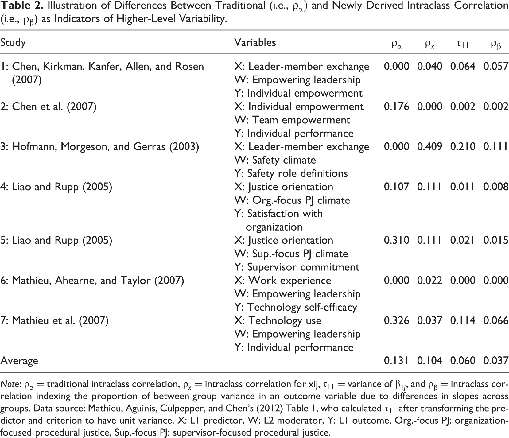
Note:
Table 2 also shows that for 2 of the 7 studies, the variance attributed to slope differences was larger than the variance associated with differences in outcome variable means as assessed by the traditional ICC (i.e.,
An additional consideration regarding results in Table 2 concerns the magnitude of ρβ. Specifically, many of the values may seem to be small—perhaps leading to the conclusion that the search for cross-level interaction effects may be futile. However, this conclusion is not warranted for the following reasons. First, LeBreton and Senter (2008) argued that ICC values of about .05 represent a small to medium effect and “values as small as .05 may provide prima facie evidence of a group effect” (p. 838). Reinforcing this recommendation, evidence made available recently demonstrates that the effect size guidelines reported by Cohen (1988) are overestimates of the types of effects usually reported in management and organizational studies research (Bosco, Aguinis, Singh, Field, & Pierce, in press). Second, ICC values should be considered within specific contexts because small observed effects may result from inauspicious designs, studies that involve phenomena leading to obscure consequences, and studies that challenge fundamental assumptions (Cortina & Landis, 2009). Third, there are numerous methodological and statistical artifacts that decrease observed effect sizes compared to their true population counterparts, and this is particularly true for interaction effects (Aguinis, 2004; Aguinis, Beaty, Boik, & Pierce, 2005; Aguinis & Stone-Romero, 1997). Accordingly, it is likely that in many cases, and due to methodological and statistical artifacts, observed variability in slopes as indicated by ρβ is actually larger in the population than has been estimated. Fourth, in some cases, small effect sizes may be practically significant (Aguinis et al., 2010). Thus, when the phenomena of interest has important implications for theory or practice, even small values for ρβ may be considered as an indication for the need to assess particular cross-level interaction hypotheses.
Comparison of ρβ With Existing Tests and Statistics
Although the recommendation in most textbooks on multilevel modeling is to rely on the traditional intraclass correlation ρα and management and organizational studies researchers seem to follow this recommendation, there are tests and indices described in the statistical and methodological literature that researchers might employ for understanding the nature of group slope differences (LaHuis, Hartman, Hakoyama, & Clark, 2014). However, ρβ offers a unique value-added contribution as an index for how group variability in slopes translates to differences in the outcome variable
Likelihood Ratio Tests of Non-Zero
Researchers could employ LRTs to statistically evaluate whether group slopes differ. Specifically, LRTs are defined as the difference between –2 log-likelihood values (–2LL) for a full and reduced model. For the current context, –2LLnull represents a random intercepts model with nonrandom slopes whereas –2LLfull allows group slopes to differ. LRTs use deviance as a test statistic where deviance = 2LLfull – 2LLnull, which is asymptotically distributed as a χ2 random variable (Aguinis et al., 2013).
It is possible to test the significance of adding a random slope to an existing random intercept model with a chi-square distribution with 2 degrees of freedom (i.e.,
An additional drawback is that the LRT test does not involve a meaningful effect size to assess the extent to which group slopes differ. Namely, LRTs serve as an omnibus test for the presence or absence of group slope differences and only provide researchers with guidance as to whether group slopes might differ in the population. In contrast, ρβ quantifies the amount of group differences in
We illustrate some of the aforementioned limitations regarding the use of null hypothesis significance testing to assess the presence of variability of slopes with data made available by Hofmann, Griffin, and Gavin (2000). We refer to this particular illustration because their chapter and data set are used by many instructors teaching multilevel modeling. In particular, a reanalysis of the Hofmann et al. data suggests a statistically significant slope variance with p < 10-6 for mood whereas
Finally, results included in Table 1 pertaining to LRT also offer additional insights regarding this test in relationship with ρβ. Specifically, Table 1 includes results based on a comparison of a full model with random intercepts and slopes to a model with only random intercepts. Statistical power for the LRT (i.e.,
Statistics Describing Group Slope Differences
There are additional strategies for interpreting the size and nature of group slope differences. These include confidence intervals and reliability coefficients for group slopes.
First, the variance of slopes could be used to gauge the degree of group slope differences in the population. Specifically,
Confidence intervals involving
As an additional approach, Raudenbush and Bryk (2002) described equations for estimating the reliability of group slopes as an index for the extent to which groups differ in

where J is the number of groups and
Referring back to Table 1, results offer additional insights regarding the reliability of slopes as an index of slope variability in relationship with ρβ. For example, Table 1 shows that the average slope reliability was approximately 0.1 in the absence of slope differences (i.e.,
Illustrative Data Set for Computing ρβ
We created a data set to illustrate the computation of ρβ. The data include the following simulated variables: “1,” which is a column of 1s, “X1” (L1 predictor), “X2” (L2 predictor), and “Y” (criterion). The R code we used for all calculations is included as a vignette in the documentation for the icc_beta R package, which can be freely downloaded through the CRAN. We make this code and data available so that they can be used for calculating ρβ for substantive as well as instructional purposes. Note that the code can be used in situations including any number of predictors. The data were simulated using the same code as for the simulation with the population model defined as:


Implementation of the R code using the illustrative data set leads to the following results and conclusions (note that we used a random-intercepts model to calculate ρα). First,
Discussion
There is an increased awareness regarding the need to understand the nature of cross-level interaction effects—the extent to which relationships at a lower-level of analysis (e.g., two individual-level variables) vary across higher-level units (e.g., groups, units, firms). This need is central for making progress in modern-day contingency theories, person-environment fit models, and any theory that considers outcomes to be a result of combined influences emanating from different levels of analysis. In addition, a better understanding of cross-level interaction effects offers information that practitioners can use in planning and implementing interventions in specific contexts because such knowledge allows them to anticipate the relative effectiveness of such interventions given certain contextual (i.e., higher-level) factors. Thus, knowledge about cross-level interaction effects allows practitioners to enhance the effectiveness of interventions. Because of these reasons, there has been an exponential growth in the literature on multilevel modeling (Aguinis, Pierce, Bosco, & Muslin, 2009; Mathieu et al., 2012), which is a data-analytic approach that considers and models data dependence and such cross-level interaction effects explicitly.
In spite of the increased diversity and complexity in the methodological literature, there is a common challenge that permeates all types of multilevel modeling: the need to understand the degree of variability of a lower-level relationship across higher-order units, processes, or contexts. Although theory-based considerations initially dictate whether multilevel modeling may be the preferred data-analytic approach, the consistent recommendation in the methodological literature is that researchers first compute the intraclass correlation, ρα, as a criterion in deciding whether to use multilevel modeling (e.g., Aguinis et al., 2013). Not surprisingly, researchers use this criterion for deciding whether the use of multilevel modeling is appropriate. If the intraclass correlation is not sufficiently high, then multilevel modeling is not considered necessary and there is also not sufficient justification for assessing cross-level interaction effect hypotheses. Inversely, multilevel modeling is the preferred approach if the intraclass correlation ρα is sufficiently high. The reason for this recommendation, which is offered in most major textbooks on multilevel modeling, is that the intraclass correlation ρα assesses the proportion of between-group variance relative to total variance in an outcome variable, and therefore, it signals the presence of nonindependence in the data structure.
Our article showed analytically and via simulation that the current conceptualization and estimation of the intraclass correlation captures across-group variability due to intercept differences and only a portion of variability attributed to slope differences. Thus, the intraclass correlation ρα is, using psychometric terminology, a deficient index of dependence. In other words, across-group variability may also exist due to slope differences across groups, but this is not reflected in the intraclass correlation as currently conceptualized and calculated. In contrast, the newly derived intraclass correlation ρβ is an index of proportion of variance in criterion scores due to group differences, but the source of this variability is group difference in slopes.
We used data reported in several articles addressing substantive theories and research domains to illustrate that using the traditional intraclass correlation ρα as an index of group differences ignores the variance attributed to group slope differences and reduces the total reported variance attributed to group differences. In some cases, using ρα as the sole criterion for understanding the degree of across-group variability may lead researchers to miss an opportunity to study cross-level interaction effects that, as noted by Mathieu et al. (2012), “lay at the heart of modern-day contingency theories, person-environment fit models, and any theory that considers outcomes to be a result of combined influences emanating from different levels of analysis” (p. 952).
There is an additional use for ρβ that has implications for future theory development. Because ρβ is expressed in standardized metric, its value is not dependent on the particular scales used in a particular study. Accordingly, similar to a Pearson’s correlation coefficient, ρβ can be used in meta-analytic reviews, and such research can open up new lines of investigation. For example, assume that a meta-analysis of the literature on the relationship between job satisfaction and task performance results in a larger mean value for ρβ compared to the estimate based on the relationship between job satisfaction and organizational citizenship behavior (OCB). This result implies that there is greater cross-level heterogeneity for the satisfaction–task performance relationship compared to the satisfaction-OCB relationship. Accordingly, this result indicates that it would be more fruitful to conduct primary-level research investigating cross-level moderating effects of the satisfaction–task performance compared to the satisfaction-OCB relationship. Alternatively, conducting meta-analyses based on ρβ values can also result in information that would be useful in terms of deciding to not search for cross-level interaction effects in certain domains. Given the proliferation of management and organizational studies theories and the need to engage in theory pruning (Leavitt, Mitchell, & Peterson, 2010), using ρβ as an index of where one should not search for cross-level interaction effects could be just as useful, or even more useful, than using it as an index of areas where such effects are more likely to be found.
In terms of yet additional uses of ρβ, our discussion thus far focused on research designs in which units are nested within collectives such as individuals within groups, groups within firms, or firms within industries. However, ρβ can also be computed within the context of longitudinal designs where repeated measurements are collected for units (e.g., individuals, firms) and time as well as time-varying predictors are included in the model. In terms of a multilevel model conceptualization, the lower level refers to observations and the higher level to the units (e.g., entrepreneurs, teams, firms) about which data have been collected over time. Referring back to Equation 10, in these types of designs, within-unit variability is captured by
Conclusion
ρα and ρβ index different sources of variance in
Footnotes
Appendix
Acknowledgment
We thank James LeBreton and two Organizational Research Methods anonymous reviewers for providing us with highly constructive and useful feedback that allowed us to improve our manuscript substantially. Also, we thank Kyle Bradley and Harry Joo for their assistance testing the icc_beta R package described in our article.
Authors’ Note
Both authors contributed equally to this research.
Declaration of Conflicting Interests
The author(s) declared no potential conflicts of interest with respect to the research, authorship, and/or publication of this article.
Funding
The author(s) received no financial support for the research, authorship, and/or publication of this article.