Integrating Moderation and Mediation

Latent Variable Interactions

While most of the published moderated mediation research to date used regression analysis to evaluate the hypothesized paths, we extend the analyses to incorporate SEM capabilities. Unlike regression models, SEM accounts for measurement error in the observed variables. Ignoring measurement errors can lead to biased parameter estimates (paths) between the variables. This issue becomes even more severe for interaction terms (Dimitruk, Schermelleh-Engel, Kelava, & Moosbrügger, 2007; Moosbrügger, Schermelleh-Engel, Kelava, & Klein, 2009) or with any estimator produced from a product term such as testing the indirect effect within mediation models (Preacher et al., 2007). However, the use of latent variables to create interaction terms within SEM creates particular challenges in this regard as outlined in the review of the five approaches to specifying latent variable interactions by Cortina, Chen, and Dunlap (2001).

When Cortina et al. (2001) was published over a decade ago, the primary difference between their reviewed approaches was how many of the observed variables from the X latent predictor variable were multiplied with the observed variables from the Z latent moderator variable to operationalize the latent interaction effect on the Y latent outcome variable. Kenny and Judd (1984), for example, stated that all pairwise product terms between the observed X and Z variables be created, whereas Jöreskog and Yang (1996) stated that only one product term between one X and one Z observed variable was required. Yet in another example, Algina and Moulder (2001) used mean centering of the indicator variables to calculate the product terms and further simplified the Jöreskog and Yang (1996) approach. Regardless of the approach, the biggest challenge associated with product terms is that they are inherently nonnormal (Cortina et al., 2001; Moosbrügger et al., 2009). Yet, estimation procedures such as maximum likelihood (ML) estimation (the primary estimation procedure in SEM) assume multivariate normality. While Cortina et al. recognized the research suggesting that ML is fairly robust in the presence of some nonnormality, they succinctly noted that “this work notwithstanding, there have been suggestions that ML will produce incorrect standard errors when the multivariate normality assumption is violated (Bollen, 1989)” (p. 326). This is due to the fact that the observed indicators of the predictor variables (the Xs) and the error/disturbance terms of the latent variables (ζ) are no longer uncorrelated and the error/disturbance terms are not normally distributed—basic assumptions within any SEM application. Besides inappropriate standard errors, other issues include having over- or underestimated values for the parameter estimates representing the main and interaction effects on the Y latent outcome variable. Excellent reviews on these and other issues (e.g., inappropriate goodness-of-fit tests, imposing multiple constraints to properly identify estimates of the product terms, etc.) using a product approach to specifying latent interaction terms and ML estimation are provided by Bollen (1989, starting p. 403), Klein and Moosbrügger (2000, starting p. 457), and Schumacker and Lomax (2000, starting p. 338).

In recognition of these issues, a number of alternative procedures for specifying latent interaction terms were developed. The earliest technique to emerge was the asymptotic distribution free estimation procedures (ADF). ADF procedures were developed as an alternative to ML estimation of the product models and included, for example, weighted least squares (WLS; Browne, 1982), mean adjusted weighted least squares (WLSM; B. Muthén, 1993), mean and variance adjusted weighted least squares (WLSMV; B. Muthén, 1993), and weighted least square with elliptical estimator (Bollen, 1989). The main advantage of ADF estimators was also one of their primary disadvantages. The advantage was in minimal assumptions about the distribution of the observed variables including the product terms among them (Bollen, 1989). However, the latter also meant that ADF estimation did not exploit the specific unique distributional properties of those variables and as such lowered the efficiency and power to estimate the parameters in which these variables are used, particularly in the presence of small sample sizes (Klein & Moosbrügger, 2000). Sample size requirements for ADF estimation are much larger than ML to achieve consistent convergence of the models (Bollen, 1989). Additionally, because these procedures are asymptotic distribution free, the computational requirements are larger than those for ML (Bollen, 1989). For example, with just 10 observed variables, WLS requires the inversion of a 55 × 55 matrix (Bollen, 1989), and the matrix grows exponentially larger with the addition of each observed variable. Even with today’s high-powered computers, it may not be feasible to estimate a model with even a moderate number of observed variables.

In light of these computational inefficiencies, the unconstrained (Marsh, Wen, & Hau, 2004, 2006) and residual centering approaches (Little, Bouvaird, & Widaman, 2006) were introduced. The unconstrained approach (Marsh et al., 2004, 2006) simplifies the approach by omitting the constraints after mean centering the indicator variables (i.e., allowing the factor loadings and error components of interaction terms to be freely estimated). The residual centering approach (Little et al., 2006) uses a two-step procedure where the indicator product terms are regressed on the X and Z variables to generate residuals, and these residuals are used as indicators of the latent interaction term in accordance with the unconstrained approach. While these approaches show promise, their ability to mitigate the nonnormality issues need further testing, and the approaches have yet to be refined enough to the point where they can be easily adopted by researchers.

Despite the excellent review provided by Cortina et al. (2001; see also Algina & Moulder, 2001), the article appeared to have little impact on researchers’ actual practices for testing interaction effects using a latent variable approach for the next decade. The vast majority of organizational science researchers throughout the first decade of the 2000s and now into the second one appear to have skipped the latent variable approach and relied primarily on a regression-based approach. Even though SEM software was readily available, the proper specification of latent interactions required using aspects of the software that was beyond the typical user’s knowledge such as identifying and properly specifying the extra constraints needed to model the parameters around the product terms and latent interaction variable. Further, there were other issues such as its computational complexity, large sample size requirements, and lack of convergence that distanced researchers even further from applying a latent variable approach to specifying interaction effects. Not surprisingly, among the 75 articles since 2008 that used a combination of moderation and mediation, all except 6 articles used regression or ANOVA based tools for testing the moderation effect, and even among those 6, only 2 used some form of latent variable interaction.

At about the same time as the Cortina et al. (2001) publication, Klein and Moosbrügger (2000) published an article on a latent variable approach to specifying interaction effects that mitigated many of the issues presented earlier and that they had been developing since the mid-1990s. Like many such new approaches, though, it was not “consumable” at that point in time because the software tools had not yet been developed to make it widely available. Further, it needed to undergo the requisite scrutiny by experts to evaluate its viability. Klein and Moosbrügger (2000) presented the LMS approach, which utilizes maximum likelihood (ML) procedures based on expectation maximization (EM) developed specifically to exploit the specific unique distributional properties of the variables in the interaction (Klein & Muthén, 2007).

Unlike other approaches, “LMS uses the raw data of indicator variables directly for estimation, and does not require the forming of any products of indicator variables” between the predictor, X, and moderator, Z, latent variables to create the latent interaction variable (Klein & Moosbrügger, 2000, p. 467). As explained succinctly in Kelava et al. (2011), LMS is a distribution analytic approach. With one major exception, the distribution analytic approach makes the same assumptions about most of the properties of the latent exogenous (predictor) and endogenous (outcome) variables (e.g., ξ and δ, ε and ζ are multivariate normally distributed with means equal to 0) as the product indicator SEM approaches reviewed by Cortina et al. (2001). The exception is an important distinguishing factor, however, between them and the LMS procedure. Specifically, based on Kenny and Judd (1984) and others, it has been demonstrated that if a significant interaction or other nonlinear term is truly present and impacting the latent endogenous (outcome) variable, η, as hypothesized, then η and its observed manifest variables (the y’s) will be nonnormally distributed (Kelava et al., 2011; Mooijaart & Satoora, 2012) in the presence of those nonlinear effects. The typical SEM approaches (product indicator) assume that η and its observed variables are normally distributed, and this is why the use of product indicator approaches to evaluate models with interactions and other nonlinear terms remains problematic (see Mooijart & Satoora, 2012, p. 65).

In contrast, the distribution analytic approaches, such as LMS, account for the nonlinearity in estimating the parameters of the model. LMS is based on the research demonstrating that much more information than just the means and covariances need to be brought into the analyses when testing for interaction effects in the models (Kelava et al., 2011; Mooijart & Satoora, 2012). To do so, LMS relies on two core statistical techniques: (a) the notion of a mixture distribution such that a nonnormal distribution may be represented by mixtures of normal distributions with different means and variances and (b) the notion of conditional distribution, which is a distribution of a variable holding one or more variables constant. As stated by Kelava et al. (2011):

To illustrate these ideas, consider the distribution of the height of adults in the United States which is nonnormal. Males have a distribution that is approximately normal (μ = 69:41, σ = 4:48 inches) and females have a distribution that is approximately normal (μ = 63:86, σ = 4:39 inches; McDowell, Fryar, Ogden, & Flegal, 2008) as well. In other words, there are two conditional normal distributions, one for gender = male and one for gender = female. Combining these two conditional distributions into one distribution represents the nonnormal distribution in the entire population. Statisticians often use this idea and combine several normal distributions to represent complex nonnormal distributions. The challenge is to find a conditioning variable like gender in the preceding example that identifies the mean and variance of the specific conditional normal distributions to be combined.

The LMS procedure builds on these two central ideas. First, although overall interaction (ξ₁ξ₂) and quadratic (ξ₁ ², ξ₂ ²) effects are nonlinear, the conditional effects are linear when a variable is controlled that causes the nonlinearity. Second, the multivariate distribution of the observed indicator variables (x₁; x₂;:::; x_q; y₁; y₂;:::; y_p) can be approximated by a weighted combination of conditionally normal distributions. For both parts, the challenge is in finding the proper variable on which to condition. (p. 473)

Here the term ξ₁ξ₂ symbolizes the interaction between two latent variables. Instead of computing product terms from the observed variables of each latent variable, LMS identifies an appropriate conditioning vector to capture the nonlinearity of moderation effects. In other words, LMS does not require creation of indicator interaction terms nor does it require the researcher to specify a conditioning variable. Instead, based on the joint vector of indicators associated with the interacting predictor latent variables, LMS procedures identifies a vector of conditioning variables using a matrix operation called Cholesky decomposition (Kelava et al., 2011). To achieve this representation, the vector of predictor variables is eventually decomposed into two vectors representing the linear and nonlinear (z1) components within both the structural and the measurement model. This z1 vector of nonlinear components is used for conditioning whereby the joint distribution of the original predictor and outcome variables is multivariate normal (Klein & Moosbrügger, 2000). The multivariate distribution of X and Y variables can be represented as a mixture distribution in which the z1 vector is used to determine the means, variances, and covariances of the set of normal distributions used in the mixture. As LMS takes into account nonnormality of interaction by representing the nonnormal distribution as a mixture of conditionally normal distributions, there is no need to specify any product terms among the indicator variables for X and Z.

Based on the z1 vector, the multivariate normal distributions of predictor and outcome variables are summed and weighted using a numeric approximation procedure (Hermite-Gaussian quadrature). To reiterate, as the nonnormality of the distribution is approximated as a mixture of conditionally normal distributions, we do not need to specify any indicator product terms. LMS uses the expectation maximization algorithm to calculate maximum likelihood estimates and standard errors for each of the parameters. LMS uses the complete raw data to calculate the parameters. Moreover, the approach generates robust estimates of the standard errors using the Fisher information matrix based on ML procedures. Thus, another advantage to LMS besides not having to specify product terms among indicators is that it provides ML estimators, and as such, “they are consistent, asymptotically unbiased, asymptotically efficient, and asymptotically normally distributed” (Klein & Moosbrügger, 2000, p. 467).

Since its introduction, the performance of the LMS approach has been evaluated in comparative studies with other approaches to specifying latent interaction terms. In one of the earliest studies, Klein and Moosbrügger (2000) compared LMS to the product indicator approach to specifying the latent interaction using WLS and normal ML estimation procedures. Along all evaluation criteria, the LMS approach was the stronger one. Similar comparative outcomes were reported by Marsh et al. (2004); Schermelleh-Engel, Werner, Klein, and Moosbrügger (2010); and Jackman, Leite, and Cochrane (2011). Jackman et al. (2011) also found that the LMS approach possessed greater power in detecting latent interaction effects. Given the favorable evaluations, the LMS approach to specifying latent interaction effects was built into the Mplus software package (L. K. Muthén & Muthén, 1998-2012) under the estimation procedure called MLR (maximum likelihood robust errors). The syntax to specify the interaction term is intuitive, typically requiring one line. Most importantly, because it does not require the user to specify product terms among the X and Z indicator variables, there is also no need to write the multitude of user-specified constraints needed to identify all of the components underlying the interaction.

Interaction effects, which by definition are nonnormal, may require larger sample sizes. In general, the sample size required to detect effects with sufficient power may depend on many factors including complexity of the model, distributions of the variables, as well as effect sizes and missing data. Based on the approach outlined in L. K. Muthén and Muthén (2002), here we provide example code of estimating sample size using Monte Carlo simulation in the context of LMS process accompanied by an Excel sheet implementing the key formulas based on L. K. Muthén and Muthén .

While relatively easy to implement, the LMS approach is not a panacea to all the challenges associated with latent variable interactions. While the LMS approach is robust to nonnormality of outcome variables, like all maximum likelihood approaches, it relies on the assumption of normality of predictor variables (Schermelleh-Engel et al., 2010). Therefore, like other nonlinear SEM approaches, the effectiveness of the approach diminishes when the sample size is small (<100), the reliability of measurements is poor (<.65), and when the predictor variables are severely nonnormal (Harring, Weiss, & Hsu, 2012). While testing certain complex moderated mediation models, when the mediator variable (M) is already influenced by an interaction of two predictor variables, M may not be normally distributed, and this can become an issue in calculating interactions involving M. As the models combining mediation and moderation get increasingly complex (e.g., multistage multi-mediator models), it is unknown at this stage how effective the LMS approach may be given that it has not been evaluated under those conditions.

LMS relies on numerical integration and raw data, allowing it to compute the conditioning vectors from the data. However, this feature also makes it a computationally intensive process. As the model gets more and more complex, the computational burden increases and may exceed the computation capacity of even the most powerful computers. Complex models may take long periods of time to come to a final solution. It has been the authors’ personal experience that when the two latent variables in the interaction term have a large number of indicators, the capacity of even our most powerful computer to derive a final solution is exceeded.

Given the computational intensity of complex moderated mediation models, researchers may start with a simpler, less complex model with a smaller number of latent variables and interactions and add to it in small steps. Additionally, it may be possible to start by estimating model parts and use those results to specify appropriate starting values for the full model. Another option would be to use parceling to reduce the number of indicators per latent variable. Before the researcher makes the choice of using parceling, our recommendation is to start with a full model using all observed variables. It is often the case, however, that a warning is received that the number of required integration points exceeds the capacity of the computer. While less frequent, the syntax will execute, but the full model may be computationally too intensive to derive a solution even when the computer is permitted to run for hours. Thus, the researcher may need to create parcels among the observed variables. Parceling is an important methodological consideration, and appropriate care must be taken to create parcels. As Little and coauthors (Little, Cunningham, Shahar, & Widaman, 2002; Little, Rehmtulla, Gibson, & Schoemann, 2013) point out, researchers need to take into account several factors, including scale type and dimensionality of the construct, to use parceling effectively. As Little et al. (2013) suggest, there are several advantages to using parceling, and while parceling can be an efficient tool, its effectiveness is dependent on the use it is put to. In the case of computational intensity of large models, the parceling may allow a researcher to test relationships that otherwise would be computationally impossible to test with the current computers. However, appropriateness of parceling in each case will depend on several factors, including dimensionality of the scale, the approach to parceling, and scale type.

It has been our experience, however, that these limitations are a function of model complexity and that under most “normal” circumstances, the LMS procedure performs as expected as and better than any other approach to specifying latent interaction terms to date. The syntax for its specification is very simple, and unlike the product-based approaches does not require the specification of any extra constraints to properly identify the parameters. It also allows the researchers to use SEM to incorporate measurement error in models that combine moderation and mediation. The following demonstrations utilize the LMS approach within the Mplus software package. Given current interest in tests of moderated mediation, the demonstration illustrates six different moderated-mediation models but from a SEM perspective.

Models and Data

We present six different models, which simultaneously combine moderation and mediation. Figures 2a through 2d illustrate the models according to Hayes’s (2013) format on the left side and according to Edwards and Lambert’s (2007) format on the right side. There are no equivalents to Hayes’s Models 21 and 11 in the Edwards and Lambert (2007) format. To demonstrate each model, we used the Edwards and Lambert (2007) fictitious example whereby feedback (predictor variable) influenced commitment (outcome variable) through job satisfaction (the mediator variable) and family centrality (continuous moderator variable) or gender (binary moderator). The first model, Hayes Model 7, illustrated in Figure 2a, is also the “First Stage Moderation model” in the Edwards and Lambert (2007) article. The second model, Hayes Model 8, shown in Figure 2b, is the model combining “Direct and First Stage Moderation effects” in Edwards and Lambert’s terminology. The third model is Hayes Model 14 (Figure 2c), which is also the “Second Stage Moderation model” in Edwards and Lambert’s terminology. The fourth model, Figure 2d, is Model 58 in Hayes’s terminology, and it corresponds to Edwards and Lambert’s “First and Second Stage Moderation model.” Model 21 (Figure 2e) from Hayes (2013) is similar to Edwards and Lambert’s “First and Second Stage Moderation model.” However, in Model 21, the first and the second path are moderated by different variables. Finally, we also demonstrate a more complex Hayes Model 11 (Figure 2f), whereby the first stage effect is moderated by two moderators. There is no equivalent to Models 11 and 21 in Edwards and Lambert’s terminology, though the equations can be extended to these models.

OPEN IN VIEWER

Figure 2.

a-f: Six illustrated models.

We tested the models using simulated data developed from the data set provided by Edwards and Lambert (2007). The original data included responses from 1,307 respondents who were surveyed on work and family issues. A full description of the variables is provided in their article. In general, though, feedback was measured with five items, satisfaction was measured with three items, commitment was measured with eight items, and family centrality was measured with six items, and all were on a 7-point response scale (1 = strongly disagree, 7 = strongly agree). Gender was coded as 0 = men and 1 = women. To create the current database, Monte Carlo simulation was used to generate 10 databases with 1,307 observations each. Given that this was a demonstration, we created a data set with three items for each scale in order to reduce model complexity. We picked one database with values most similar to the original data set.

Given that much of the following is illustrating how to conduct the analyses with more focus on syntax than the actual outcomes, only the analyses of Hayes Model 7 (First stage moderation), and Hayes Model 11 are illustrated in the following sections. We limited it to these two models simply because there is a great deal of repetition from one model to the next. The analyses of all of the remaining models except 11 are sufficiently similar to Model 7 that the reader should be able to understand the differences in syntax by examining the syntax files for those other models. Model 11, though, is sufficiently different because it encompasses a three-way latent variable interaction. Therefore, it warrants separate attention. All the sample data and code are accessible at https://drive.google.com/#folders/0BypX-E-3GQYxSVBBQ1JpX29WbUE.

The latent variable interactions were defined using the XWITH statement in Mplus syntax. The XWITH option in Mplus needs to be used with TYPE=RANDOM and ALGORITHM=INTEGRATION to define latent variable interactions. XWITH option is not limited to only latent variable interactions and can also be used to define interactions between latent and observed variables, both binary and continuous. XWITH is paired with the symbol | to define the interaction variables. We then calculate the indirect and total effect based on equations from Edwards and Lambert (2007) using model constraint statements in Mplus. Since all the effects are calculated using the MLR estimator (the LMS estimation) in Mplus, the standard errors are known to be robust.

Analysis of Hayes Model 7—First Stage Moderation Model

As seen in Figure 2a, this model specifies that feedback (X) influences commitment (Y) via an indirect effect through satisfaction (M), and centrality moderates the relationships between feedback and satisfaction. This model is akin to Model 7 in Hayes (2013) and the First Stage Moderation model in Edwards and Lambert (2007).

To specify latent variable interactions, we need to use the following Mplus commands before specifying the measurement and path models. Per the explanation in the introduction, underlying the LMS approach is a numerical integration process, and these lines of syntax are the ones that evoke it.

ANALYSIS:

TYPE = RANDOM;

ALGORITHM = INTEGRATION;

As with all SEM models, the first step is to define the latent variables using a measurement model. This required the four lines of code in the following, where the provided names for the latent variables (e.g., fbk, sat, etc.) are to the left of the “by” command and the corresponding observed variables underlying each latent variable is to the right. The letter following the exclamation mark is a reminder as to which variables were the X, M, Y, and W.

fbk BY feed1-feed3; ! X

sat BY sat1-sat3; ! M

com BY commit1-commit3; ! Y

cen BY cent1-cent3; ! W

Specifying the actual latent variable interaction between feedback and centrality in the model is completed using the XWITH command.

fbkccenc | fbk XWITH cen;

The term fbkcenc is the label the user gives to the latent interaction variable. The pike key (|) is the Mplus command denoting that the latent interaction is defined by the terms to the right of it. Specifically, that the latent variable fbk is to be crossed with (XWITH) the other latent variable cen, both of which were defined in the measurement model.

Again, as with all SEM models, the next step is to test the proposed path model. For the main effects, the structural path model was estimated by regressing satisfaction (M) on feedback (X) and centrality (W) and commitment (Y) on feedback (X) and satisfaction (M).

sat ON fbk;

sat ON cen;

com ON sat;

com ON fbk;

Testing the effect of the latent interaction term is also simply done with an “ON” statement. Specifically, the following line of syntax was used:

sat ON fbkccenc (axw5);

Assuming the reader is looking at the actual syntax file while following this text, you will notice two other major characteristics about the file. First, many of the lines of syntax are followed by parenthetical markers such as the (axw5) in the previous line. Recall that we mapped the models onto the equations presented by Edwards and Lambert (2007). The axw5 is the latent interaction effect per Equation 5 from Edwards and Lambert (2007). In this manner, the user can go to their article and see what value belongs to the many functions underlying their equations. Following an estimated parameter with parentheses in Mplus assigns the obtained value to that marker.

The aforementioned is important because of the second major characteristic of the syntax files. Namely, using the MODEL CONSTRAINTS feature of Mplus permits the user to create new terms and values. As can be seen in the syntax, we used the constraints for two primary purposes. The first was to execute the Edwards and Lambert (2007) equations and test the differences between low and high values of the moderator. In the case of Model 7, this was the difference in First Stage Moderation at the low and high values of the moderator. The second purpose was to calculate the predicted values at the low and high values of the moderator so that we could plot the interaction. Table 3 shows results for all the calculated effects. A few example lines of syntax from the main syntax file illustrating each of these two purposes are presented in Table 4, and the plots for Model 7 are illustrated in Figure 3.

OPEN IN VIEWER

Table 2.

Fit Indices and Unstandardized Coefficients for All Models.

	Model 7		Model 8		Model 14		Model 58		Model 21		Model 11
	Baseline	Interaction	Baseline	Interaction	Baseline	Interaction	Baseline	Interaction	Baseline	Interaction	SEM Baseline	Interaction
χ2	40.21		39.308		169.62		39.308		51.324		52.09
df	49.00		48		49		48		60		60
p	0.81		0.81				0.81		0.7800		0.75
Log likelihood	–23,527.43	–23,522.98	–23,526.98	23,522.48	–23,587.64	–23,596.84	–23,527.00	–23,522.26	–23,525.71	–23,520.31	–23,526.10	–23,518.57
Scaling correction		0.99		0.994		1.01		1.05		1.11		0.98
Estimated pathsa	41	43	42	41	41	43	42	45	41	45	42	48
Comparative Fit Index	1.00				0.983		1.00		1.00		1.00
Tucker-Lewis Index	1.00				0.977		1.00		1.00		1.00
Root mean square error of approximation	0.00		0.00		0.042		0.00		0.00		0.00
Standardized root mean square residual	0.01		0.01		0.05		0.01		0.015		0.02
Akaike Information Criterion	47,136.87	47,131.97	47,137.97	47,134.97	47,257.27	47,279.67	47,137.97	47,134.53	46,995.35	47,130.61	47,136.19	47,279.67
Bayesian Information Criterion	47349.06	47354.51	47355.34	47367.86	47469.47	47502.216	47355.34	47367.42	47212.71	47363.51	47,353.56	47,502.22
X→ M	0.99**	0.99**	0.99**	0.99**	1.02**	1.03**	0.99**	0.72	0.99**	0.78	0.99**	1.00**
W→M	0.52***	0.51**	0.52**	0.50**			0.52**	0.50**	0.52**	0.50**	0.53**	0.56**
XW→M		–0.20**		–0.20**				–0.20**		–0.20**	–0.10	–0.1
X→Y	0.36**	0.36**	0.37**	0.37**	0.37**	0.37**	0.37**	0.38**	0.35**	0.35**		–0.16*
M→Y	0.61**	0.61**	0.59**	0.59**	0.59**	0.57**	0.60**	0.56**	0.61**	0.60**		–0.10
W→Y			0.05	0.05			0.05	0.03				–0.20
XW→Y				0.01
MW→Y								–0.02				–0.17
V→Y					0.05	0.05			0.01	0.14	0.36**	0.36**
MV→Y						–0.03				0.07	0.61**	0.61**

Note: N = 1,307. All the coefficients are unstandardized.

^aThe term estimated paths refers to number of free parameters in the output. Including the option TECH1 on the output line also gives more detailed information on the number of parameters estimated.

**p < .01.

OPEN IN VIEWER

Table 3.

Direct, Indirect, Total Effects for the Models.

	First Stage	Second Stage	Direct	Indirect	Total
Model 7 (First Stage moderation)
Low centrality	1.13**			0.68**	1.04**
High centrality	0.85**			0.52**	0.88**
Difference	0.27**			0.17**	0.17**
Model 8 (direct effects and First Stage Moderation)
Low centrality	1.03**		0.37**	0.67**	1.03**
High centrality	0.85**		0.39**	0.50**	0.89**
Difference	0.27**		–0.02	0.16**	0.14
Model 14 (Second Stage Moderation)
Low centrality		0.60**		0.62**	0.99**
High centrality		0.55**		0.57**	0.95**
Difference	0.00	0.04		0.05	0.05
Model 21 (First and Second Stage Moderation)
Low centrality	1.12**			0.67**	1.02**
High centrality	0.85**			0.75**	0.86**
Difference	0.27**			–0.08	0.16** (M) and 0.18** (W)
Men		0.60**		0.51	1.10**
Women		0.67**		0.57	0.92**
Difference		–0.07		–0.06	–0.08 (L) and –0.06 (H)
Model 58
Low centrality	1.12**	0.60**		0.68**	1.05**
High centrality	0.85**	0.58**		0.49**	0.87**
Difference	0.27**	0.03		0.19*	0.19*
Model 11
Low centrality
Men	1.12**			0.68**	1.48**
Women	1.18**			0.71**	1.54**
High centrality
Men	0.91**			0.55**	1.27**
Women	0.68**			0.41**	1.04**
Difference
Men	0.22*			0.13*	0.22*
Women	0.49*			0.30**	0.49**

Note: N = 1,307. All the coefficients are unstandardized.

*p < .05. **p < .01.

OPEN IN VIEWER

Table 4.

Model Constraint Command Examples for Calculating Effects and Plotting Points.

	First Stage	Plotting Values
Model 7	hiFirst = (ax5 + (axw5*hiw));	HFprimL = Hi1stInt + (HiFirst*fdbkone); HFprimH = Hi1stInt + (HiFirst*fdbksev);
	loFirst = (ax5 + (axw5*Low));	LFprimL = lo1stInt + (LoFirst*fdbkone); LFprimH = lo1stInt + (LoFirst*fdbksev);
	FirstDiff = lofirst - hifirst;
Model 11	lo1First = (ax5 +(axz5*loZ)+ (axw5*low) + (awz5*low*loz));	L1FprimL = lo1Int + (Lo1First*fdbkone); L1FprimH = lo1Int + (Lo1First*fdbksev);
	hi1First = (ax5 +(axz5*loZ)+ (axw5*hiw) + (awz5*hiw*loz));	H1FprimL = Hi1Int + (Hi1First*fdbkone); H1FprimH = Hi1Int + (Hi1First*fdbksev)
	lo2First = (ax5 +(axz5*hiZ)+ (axw5*low) + (awz5*low*hiz));	L2FprimL = lo2Int + (Lo2First*fdbkone); L2FprimH = lo2Int + (Lo2First*fdbksev);
	hi2First = (ax5 +(axz5*hiZ)+ (axw5*hiw) + (awz5*hiw*hiz));	H2FprimL = Hi2Int + (Hi2First*fdbkone); H2FprimH = Hi2Int + (Hi2First*fdbksev);

OPEN IN VIEWER

Figure 3.

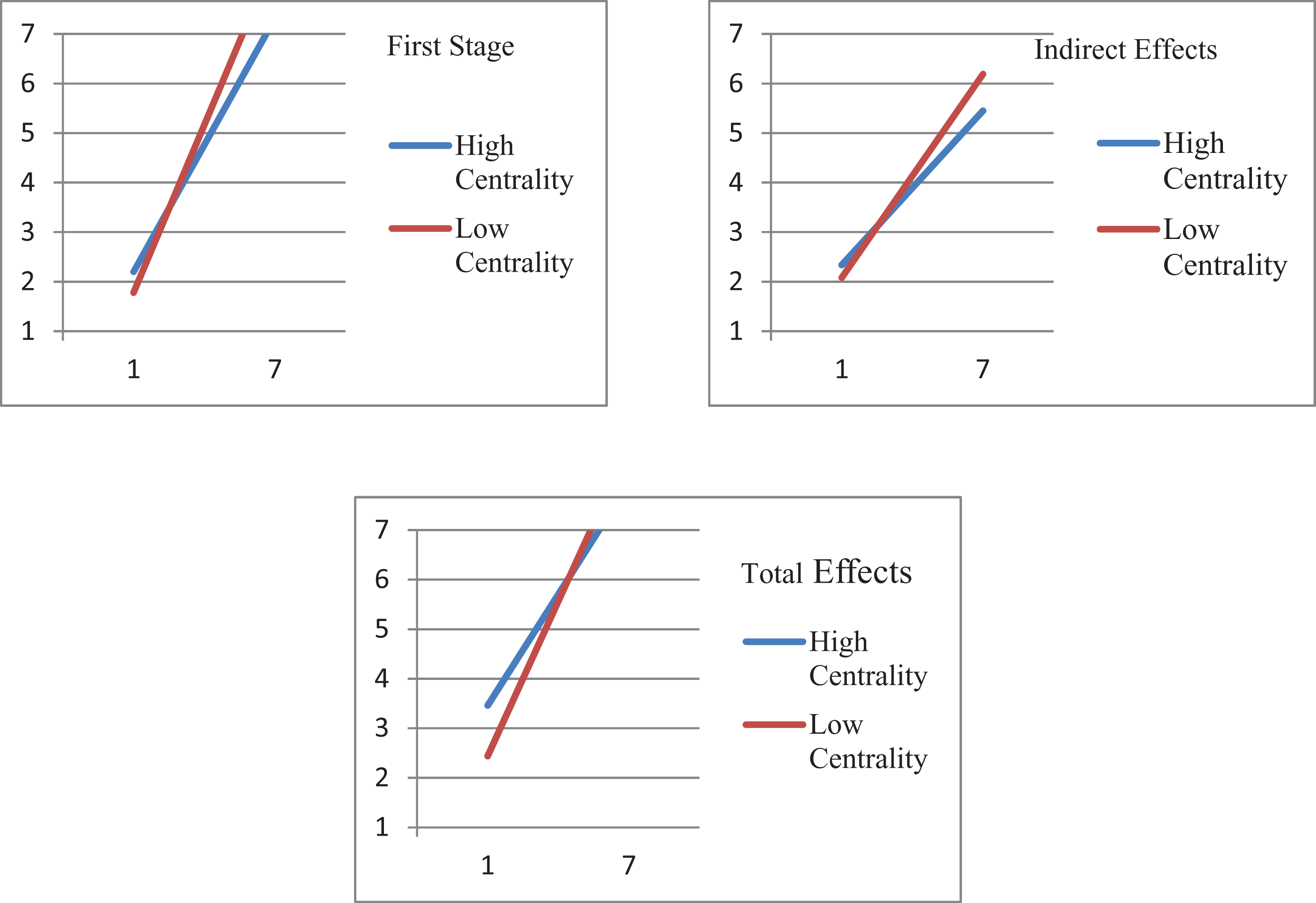
Model 7 first stage, indirect and total effects.

We are optimistic that by studying the Hayes Model 7 (Edwards and Lambert first-stage moderation only model) syntax file along with the notes we provide in that file, the reader should be able to follow the changes in syntax the represent the other models. For example, the primary difference between Hayes Model 7 and Hayes Model 58 (the first- and second-stage moderation model) is the additional syntax to operationalize the second-stage moderation effect and to generate the values for plotting that interaction. Similarly, the Hayes Model 14 (Edwards and Lambert second-stage only moderation model) excludes the syntax for first-stage moderation and only includes that for second-stage moderation. While it may take some effort to understand the syntax itself, every attempt was to take a modular approach so that the operationalization of different stages or the full model are readily apparent.

Analysis of Hayes Model 11—Two Moderators for the First Stage Effect Only

This model has no equivalent in the Edwards and Lambert (2007) article. It specifies that feedback (X) influences commitment (Y) via an indirect effect through satisfaction (M), centrality (W) moderates the relationship between feedback (X) and satisfaction (M), and gender (Z) moderate the relationships between centrality (W) and satisfaction (M) such that there is a three-way interaction between X, W, and Z. This model is illustrated in Figure 2f.

For Model 11, the measurement model was the same as previously described. The latent variable interactions differ from the previous model in that there are two-way interactions (the first three lines of syntax in the following) in addition to the theoretical three-way interaction (the last line of syntax in the following).

fbkccenc | fbk XWITH cen; ! XW

fbkcgen | fbk XWITH gen;! XZ

cencgen | cen XWITH gen;! WZ

fbkcengen |fbkccenc XWITH gen;! XWZ

Note that the interaction of a binary variable (gender) with a latent variable is defined the exact same way we define interactions between two latent variables.

As the next step, we provide syntax to test the proposed path model. For the main effects, the structural path model was estimated by regressing satisfaction (M) on feedback (X), centrality (W), and gender (Z) and commitment (Y) on feedback (X) and satisfaction (M).

sat ON fbk (ax5);

sat ON cen (aw5);

sat ON gen (az5);

com ON fbk (bx20);

com ON sat(bm20);

Testing the effect of the latent interaction term is also simply done with an “ON” statement. Specifically, the following lines of syntax were used to test the effects of the two-way interactions (the first three lines of syntax in the following) in addition to the theoretical three-way interaction (the last line of syntax in the following).

sat ON fbkccenc (axw5);

sat ON fbkcgen (axz5);

sat ON cencgen (awz5);

sat ON fbkcengen (axwz5);

Similar to the Model 7 file, we use parenthetical markers such as the (axw5) in the previous lines that are extensions of the Edwards and Lambert (2007) notations to the current model. Following an estimated parameter with parentheses in Mplus assigns the obtained value to that marker. We then used the markers and manipulated them using the MODEL CONSTRAINTS feature of Mplus to create new terms and values. Similar to the previous example, we used the constraints for two primary purposes, to execute the extensions based on the Edwards and Lambert (2007) equations and test the differences between low and high values of the moderator. Table 3 shows results for all the calculated effects. A few lines of syntax illustrating each of these two purposes are presented in the bottom half of Table 4, and the plots for Model 11 are illustrated in Figure 4.

OPEN IN VIEWER

Figure 4.

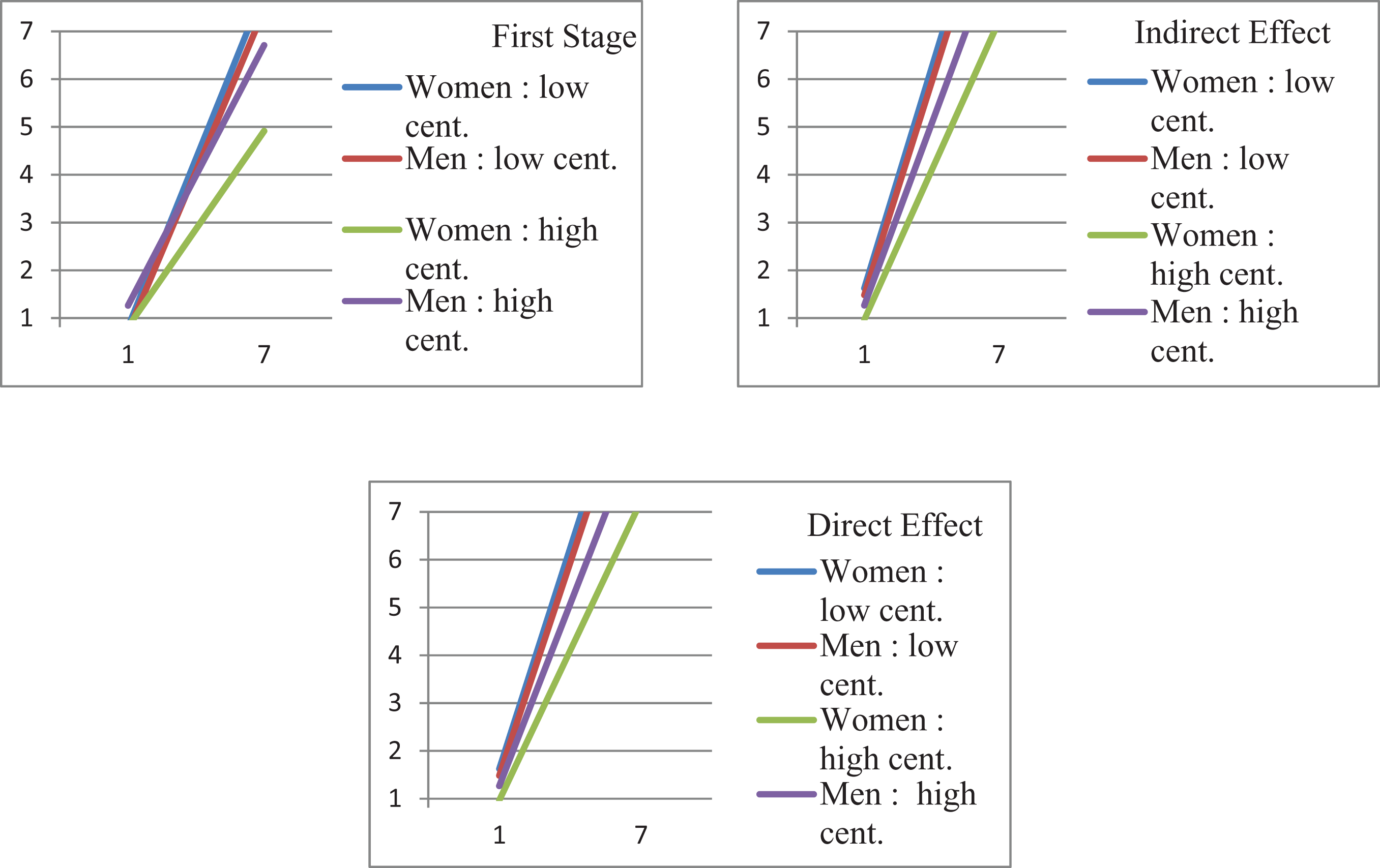
Model 11 first stage, indirect and total effects.

Interpreting Moderation

Similar to regression-based moderation approaches, a significant interaction term indicates that the effect of the key independent variable on the dependent variable differs across the range of the moderator. It can be further probed by investigating if the coefficients, which represent slopes of the relationship between independent and dependent variable, differ across different values of the moderator. In our case, moderation of first, second, direct, indirect, and total effects means that these paths may differ at different levels of the moderator. Based on Edwards and Lambert (2007), these effects can be calculated at different values of the moderator. Overall, interpretation of moderation will be based on (a) statistical significance of the interaction term and (b) statistical significance of the difference values of first, second, direct, indirect, and total effects. Further, simple slopes for each path and effect can be plotted. We provide code for plotting all the effects based on the Edwards and Lambert (2007) paper. Further, based on the graphing capabilities in Mplus, we also provide simple code for plotting indirect effects.

Endogeneity and Calculation of ρ

As Antonakis, Bendahan, Jacquart, and Lalive (2010) point out, endogeneity is an important consideration in understanding mediation models. The point 9 in their 10 commandments recommends that researchers calculate correlations between the disturbances of the mediator and the outcome variable. Similarly Imai, Keele, and Tingley (2010) and Imai, Keele, and Yamamoto (2010) point out that correlation between the mediator and outcome variable (in the example case, satisfaction and commitment) can be treated as a sensitivity parameter to violation of the sequential ignorability assumption of causal mediation. Under the sequential ignorability assumption, the correlation between mediator and outcome disturbance terms (ρ) should be 0. In our model, it is very easy to calculate ρ by adding one line of code:

sat with com;

Tables 5 and 6 list results for the models, which include estimation of the correlation between the disturbances of mediator and the outcome variable (satisfaction and commitment). Estimating such a parameter may not always be possible given the identification issues, and some models may not converge when the correlation between disturbances of mediator and outcome variables are estimated. We found that for some models, including the correlation between residuals of the mediator and outcome variable produced errors and inconsistent estimates (e.g., Model 14), which may indicate potential model misspecification. However, since the purpose of this paper is to illustrate how the models could be adapted, we have included the results in this paper. For substantive papers, it is important to specify appropriate models.

OPEN IN VIEWER

Table 5.

Fit Indices and Unstandardized Coefficients for All Interaction Models After Correlating Disturbances of M and Y.

	Model 7	Model 8	Model 14	Model 21	Model 58		Model 11
Log likelihood	–23,522.606	–23,522.49	–23,596.6	–23,519.96	–23,521.92	Log likelihood	–23,518.4
Scaling correction factor	0.99	0.96	1.01	1.13	1.02	Scaling correction factor	0.98
Estimated pathsa	44	46	44	46	46		49
Akaike Information Criterion	47,133.213	47,136.98	47,281.18	47,131.92	47,135.84	Akaike Information Criterion	47,134.871
Bayesian Information Criterion	47,360.934	47,375.05	47,508.9	47,370	47,373.91	Bayesian Information Criterion	47,388.47
X→M	0.99**	0.98**	1.03**	0.69**	0.86**	X→M	1.01**
W→M	0.51**	0.51**		0.50**	0.50**	W→M	0.56**
XW→M	–0.20**	–0.20**		–0.20**	–0.20**	Z→M	–0.09 (ns)
X→Y	0.23**	0.64**	1.61 (ns)	0.29**	0.73 (ns)	XW→M	–0.16**
M→Y	0.67**	0.32**	–0.62 (ns)	0.65**	0.20 (ns)	XZ→M	–0.09 (ns)
W→Y		0.18**	0.05 (ns)		0.21 (ns)	WZ→M	–0.21 (ns)
XW→Y		–0.04 (ns)	–0.03 (ns)			XWZ→M	–0.17 (ns)
MW→Y					–0.05 (ns)	X→Y	0.32**
V→Y				0.16(ns)		M→Y	0.64**
MV→Y				0.07 (ns)
M<→Y	–0.05 (ns)	0.17**	0.93 (ns)	–0.05 (ns)	0.23 (ns)	M<→Y	–0.03 (ns)

Note: N = 1,307. All the coefficients are unstandardized.

^aThe term estimated paths refers to number of free parameters in the output. Including the option TECH1 on the output line also gives more detailed information on the number of parameters estimated.

**p < .01.

OPEN IN VIEWER

Table 6.

Direct, Indirect, Total Effects for All Models After Correlating Disturbances of M and Y.

	First stage	Second stage	Direct	Indirect	Total
Model 7
Low centrality	1.12**			0.75**	1.05**
High centrality	0.86**			0.57**	0.87**
Difference	0.27**			0.18**	0.18**
Model 8
Low centrality	1.13**		0.67**	0.36**	1.03**
High centrality	0.85**		0.62**	0.28**	0.89**
Difference	0.28**		0.05 (ns)	0.09**	0.14 (ns)
Model 14
Low centrality		–0.60 (ns)		–0.62 (ns)	0.99**
High centrality		–0.64 (ns)		–0.66 (ns)	0.95**
Difference		0.05 (ns)		0.05 (ns)	0.05 (ns)
Model 21
Low centrality	1.12**			0.73**	1.03**
High centrality	0.85**			0.81**	0.85**
Difference	0.27**			–0.08	0.18** (M) and 0.20** (W)
Men		0.65**		0.56	1.11**
Women		0.73**		0.62	0.91**
Difference		–0.07 (ns)		–0.06	–0.08 (ns) (L) and –0.06 (ns) (H)
Model 58
Low centrality	1.12**	0.27 (ns)		0.30 (ns)	1.02**
High centrality	0.85**	0.20 (ns)		0.17 (ns)	0.90**
Difference	0.27**	0.07 (ns)		0.13 (ns)	0.13 (ns)
Model 11
Low centrality
Men	1.12**			0.72**	1.45**
Women	1.18**			0.76**	1.51**
High centrality
Men	0.91**			0.58**	1.23**
Women	0.69**			0.44**	1.01**
Difference
Men	0.22*			0.14*	0.22*
Women	0.50*			0.32**	0.50**

Note: N = 1,307. All the coefficients are unstandardized.

*p < .05. **p < .01.

Model Fit Involving Latent Variable Interaction

When using the LMS approach within Mplus the first time, the user will see that none of the “typical” fit indices are reported such as the chi-square goodness of fit, Tucker-Lewis Index (TLI), Comparative Fit Index (CFI), and the like. Rather, only the information criteria, Akaike Information Criterion (AIC), Bayesian Information Criterion (BIC), and sample adjusted BIC (SABIC), are reported. The “typical” fit indices are based on normal theory, and as explained previously, the LMS approach is not. The developers of Mplus recognized this and purposely did not program those fit indices in to avoid giving the impression that they are accurate and okay to use. One method to get a sense as to how well the model would fit is to run a baseline model where the moderator is included, but only its main effects are specified (paths from it to the dependent variable), and the model is evaluated using the traditional maximum likelihood estimation procedure; that is, the latent interaction term (using the XWITH statement) is not included. It is after this then that the model with the latent interaction term is estimated. One can then compare the latter interaction model to its baseline using the information criteria. In most cases, the fit of the baseline model should meet all of the usual criteria for judging a well-fitting model. If it does not fit well, then adding the interaction to it does not make sense. Assuming it fits well, one can then evaluate whether the inclusion of the interaction term changes the information criteria between the baseline and interaction models. When hypothesizing a disordinal interaction, it is likely that the baseline structural model may not fit very well, in spite of a good measurement model. In such cases, addition of the latent variable interaction model dramatically reduces the information loss, leading to a smaller information criteria numbers.

In practice we prefer, and therefore recommend, the AIC over the BIC for these comparisons (Vandenberg & Grelle, 2009). Both Burnham and Anderson (2002) and Yang (2005) demonstrate that the BIC is based on some unrealistic assumptions and over-penalizes for the inclusion of more parameters. For example, the BIC assumes that the population of alternative models for a given model is known when that is rarely if ever the case within the organizational sciences (Vandenberg & Grelle, 2009). Also, the AIC is asymptotically optimal, the BIC is not, in identifying the model with the smallest or least mean square error under the commonly made assumption that the true population model is infinite dimensional (Yang, 2005). Infinite dimensionality is not an unreasonable assumption as it implies that the processes that generate the data are rarely represented exactly by a fixed finite dimensional model (Kuha, 2004). While the absolute values of AIC are not useful for interpretation, the differences in the AIC values of different models are of key importance (Burnham & Anderson, 2002). Ideally, the model with the smallest AIC is selected as the optimal one as larger AIC indicates larger information loss.

However, we would like to interject a word of caution in that the goal here is not about finding the optimal model from among a number of alternatives. Rather, the goal is simply to ask whether the inclusion of the latent interaction term with its paths to other variables results in a dramatic loss of information relative to the baseline, namely, increases the value of AIC. Further, the AIC does penalize for model complexity, and the inclusion of the interaction terms increases model complexity a great deal. While comparing AIC values, the smaller value is preferred over the larger value. According to Burnham and Anderson (2002), difference in the AIC (Δ_i = AIC_i – AIC_min) can be very important and useful in determining the better model. Δ_i = 4 – 7 can indicate that the model with smaller AIC is considerably better fitting, and Δ_i > 10 can rule out the worse fitting model. One sees this in Table 2, where all of the interaction models except Models 21 and 11 had smaller AIC values than the baseline models. Models 21 and 11, however, were the most complex interaction models in the set tested. Thus, their respective AIC values were larger than those of their respective baseline models. Further, in Table 5, which tested the same models after including the correlation of disturbances of outcome and mediator, Model 14 showed inconsistent estimates and also a poorer fit index (high AIC) as compared to other models, flagging the model misspecification. Maslowsky, Jager, and Hemken (2015) recently proposed another method for evaluating the fit of the model with the latent interaction variable. Like the previous approach, the relative contribution of the latter model is compared to a baseline model without the latent interaction variable. However, instead of comparing the AIC values from both models, Maslowsky et al. recommend the log-likelihood ratio test; that is, computing the difference between the log-likelihood functions from both models and treating the difference as a chi-square value.

Bootstrapping

In the older versions of Mplus, it was not possible to bootstrap the latent variable interaction models. However, the more recent 7.2 version of Mplus also allows the users to use ML estimator and bootstrapping. In our analysis, the confidence intervals from both the processes were identical. While the bootstrapped processes take a lot longer to run, many researchers may prefer bootstrapped results. To bootstrap the latent variable interaction models, it needs two additional lines of syntax to specify the estimator and the number of bootstrap draws. So the analysis syntax now would be:

ANALYSIS:

TYPE = RANDOM;

ALGORITHM = INTEGRATION;

ESTIMATOR = ML;

BOOTSTRAP = 500;

PROCESSORS = 4;

To generate the bootstrapped output, we also specify one additional syntax command in the output line:

OUTPUT: samp CINTERVAL (BCBOOTSTRAP);

Both LMS and bootstrapping are computationally intensive, and therefore it may take several hours for a bootstrapped complex moderated mediation model to run and generate output. However, depending on how many core processors your own computer has, processing speeds can be dramatically increased by instructing Mplus to use all of the computer’s core processors by inserting the PROCESSORS = command.