Bias and Precision of Alternate Estimators in Meta-Analysis: Benefits of Blending Schmidt-Hunter and Hedges Approaches

Abstract

We describe a new estimator (labeled Morris) for meta-analysis. The Morris estimator combines elements of both the Schmidt-Hunter and Hedges estimators. The new estimator is compared to (a) the Schmidt-Hunter estimator, (b) the Schmidt-Hunter estimator with variance correction for the number of studies (“k correction”), (c) the Hedges random-effects estimator, and (d) the Bonett unit weights estimator in a Monte Carlo simulation. The simulation was designed to represent realistic conditions faced by researchers, including population random-effects distributions, numbers of studies, and skewed sample size distributions. The simulation was used to evaluate the estimators with respect to bias, coverage of the 95% confidence interval of the mean, and root mean square error of estimates of the population mean. We also evaluated the quality of credibility intervals. Overall, the new estimator provides better coverage and slightly better credibility values than other commonly used methods. Thus it has advantages of both commonly used approaches without the apparent disadvantages. The new estimator can be implemented easily with existing software; software used in the study is available online, and an example is included in the appendix in the Supplemental Material available online.

Keywords

meta-analysis bias efficiency coverage credibility interval

Meta-analysis refers to statistical techniques that combine the quantitative results of empirical studies, that is, effect sizes. There are many different effect sizes that can be combined in a meta-analysis (Borenstein, Hedges, Higgins, & Rothstein, 2009; Lipsey & Wilson, 2001), and there are several different techniques or methods in which the effect sizes can be combined (Bonett, 2008; Raudenbush, 2009; Schmidt & Hunter, 2015; Viechtbauer, 2010). Research on methods of meta-analysis is important because systematic reviews using meta-analysis tend to be quite influential (DeGeest & Schmidt, 2010), so methods that provide better estimates or better inferences are to be preferred.

In psychological research, several different statistical approaches have been used to estimate the overall mean effect size (Shadish & Haddock, 2009; Viechtbauer, 2010). However, there are two approaches that appear dominant in the current literature (Field & Gillett, 2010). We will label these (a) Schmidt-Hunter (Schmidt & Hunter, 2015) and (b) Hedges (Borenstein et al., 2009; Hedges & Olkin, 1985; Hedges & Vevea, 1998). Furthermore, in psychological research, the dominant effect sizes appear to be the correlation coefficient (Pearson’s r) and the standardized mean difference (Cohen’s d). The correlation coefficient is the focus for this article because it is the modal effect size found in organizational research.

The statistically appropriate method for meta-analysis of the correlation coefficient has been somewhat controversial. Here we sketch some of the arguments; the interested reader is directed to Schmidt and Hunter (2015) and Borenstein et al. (2009) for details. Hedges and Olkin (1985) showed that the optimal weights in meta-analysis depend on the magnitude of both the within-study and between-study variances. When the between-study variance is absent (the common effect model; the random-effects variance is zero), only the within study variance need be considered, and studies with a smaller sampling variance should receive greater weight. Unfortunately, the sampling variance of the correlation coefficient depends on the population parameter:

σ_{e i}^{2} ≅ \frac{{(1 - ρ^{2})}^{2}}{N - 1} .

Thus, an exact calculation of the (inverse variance) weights for correlation coefficients requires knowledge of the unknown underlying parameter.

Although an exact solution to the weights is not possible using the formula for the variance of the correlation, one approach to estimating weights is to substitute the sample value of r for ρ. Because r is not estimated well unless the sample size is large, such an approach does not work well with small samples and is not recommended (Schulze, 2007). A second approach is to replace ρ with the sample-weighted mean r across studies (Schmidt & Hunter, 2015). Because the weighted mean r is constant across studies in the Schmidt-Hunter (2015) analysis, it drops out of the weights (although it figures in subsequent calculations). A third approach is employ the Fisher r-to-z transformation, which eliminates the parameter ρ from the calculation of the sampling variance (Borenstein et al., 2009). A fuller description of each of the approaches along with pros and cons of each is presented in the section on models.

In addition to within-study variance, meta-analyses in organizational research also commonly find between-study variance, that is, variance in effect sizes after accounting for sampling error and other artifacts (Paterson, Harms, Steel, & Credé, 2016). In cases where the random-effects variance is positive, the optimal (consistent and efficient) weights should incorporate the random-effects variance component as a second source of uncertainty (along with the within-studies variance; Hedges & Olkin, 1985; Hedges & Vevea, 1998). Although some meta-analysis computer programs incorporate the between-studies variance into the calculation of the weights (e.g., Viechtbauer, 2010), the software mentioned in Schmidt and Hunter (2015) does not.

The optimal weights are a function of the population value of the random-effects variance component, which like the value of ρ, is unknown (Raudenbush, 2009). Schmidt and Hunter’s (2015) rationale for excluding the between-study variance in the weights is that the between-study variance is poorly estimated, especially when the number of studies is small; the use of the between-studies variance is justified by large-sample statistical theory. The poor estimation of between-studies variance is thus likely to produce inaccurate weights and poorer estimates of the overall mean effect size. Schmidt and Hunter (2015) cited Monte Carlo studies that have shown superior results for sample size weights over weights that include random-effects variance for correlation coefficients (Brannick, 2006; Schulze, 2004). Thus, one difference between the Schmidt-Hunter estimator and the Hedges estimator is whether the random-effects variance component is included in the study weights.

We concur that the between-studies variance is often poorly estimated, particularly when the number of independent effect sizes is small. However, the purpose of including the between-studies variance is to make the weights closer to unit weights as the between-studies variance increases; unit weights would be the asymptotic limit in which all the variance was between studies. For ordinary meta-analyses, the impact of including the between-studies variance is to flatten the weights; the reduction in variance in weights across studies will depend on the magnitude of the within-study and between-study variances. When there is random-effects variance in a population of studies, incorporating its estimate in the weights is theoretically justified because by chance a very large N study may be unrepresentatively large or small in magnitude of ρ_i; in such cases the meta-analytic mean will deviate from the population value (Bonett, 2008).

In simulations, unit weights have worked surprisingly well, even though they do not follow statistical optimality (Bonett, 2008, 2010). For example, Brannick, Yang, and Cafri (2011) found that although the Schmidt-Hunter approach worked best overall for the effect size r, unit weights actually worked better than Schmidt-Hunter weights in estimating the overall mean effect size when the between-study variance was large and sample distributions were taken from meta-analyses in applied psychology. Therefore, it is possible that including the estimated random-effects variance in the weights is helpful even if such variance estimates are not very accurate.

The Morris estimator (which we introduce subsequently), uses both the sample-weighted mean r (like Schmidt and Hunter) and the random-effects variance (like Hedges) in the estimation of the meta-analytic mean. Our specific aim was to compare the Morris estimator to the other estimators to determine whether the Morris estimator appears preferable in computing summary effects, confidence intervals, and credibility intervals in organizational research.

The r to z Controversy

Another important difference between the Schmidt-Hunter and Hedges estimators is whether to use the r to z transformation. Although Fisher’s z eliminates parameter ρ from the computation of the weight, Schmidt and Hunter (2015) stated that the negative bias in average r is always less than the positive bias in average z (p. 66) and thus r is preferred to z for meta-analysis. Although other authors have argued that z is appropriate to use when averaging values of the correlation coefficient (Corey, Dunlap, & Burke, 1998; James, Demaree, & Mulaik, 1986; Silver & Dunlap, 1987), Schulze (2004) showed that as random-effects variance increases, use of the transformation provides increasingly inaccurate results.

For example, suppose we have two subpopulations, one with ρ = .6 and one with ρ = .8. The overall mean of the two is .7, which is presumably the value that the researcher wishes to estimate. If we convert each of these to Fisher’s z, we find that z (.6) = 0.69, z (.8) = 1.10, and the mean of the two, when retranslated back to r, is .71 rather than .7 (Schulze, 2004). If all the observed correlations are small, the magnitude of the difference will be trivial, but if some are large, the difference can be an issue.

A second complication is that the random-effects variance component computed in z is not directly comparable to the original units, which poses problems for interpretation. The square root of the random-effects variance component can be loosely interpreted as the average distance of the local study from the grand mean. Such an interpretation holds (approximately) if the analysis is computed in the original metric. When the analysis is computed in z, the interpretation no longer holds. We can still find confidence and credibility values in z and then translate those back to r, but the square root of the random-effects variance will be in the metric of z, not r (Borenstein et al., 2009).

Other researchers have proposed integral methods of retranslation of z to r, which they claim to largely solve the problems of bias in the estimate of the mean (Hafdahl & Williams, 2009; Law, 1995) and comparability of the estimate of the random-effects variance (Law, 1995; Steel, 2013). However, the integral method does not appear to have been implemented in widely available software and empirical comparisons in the literature may not correspond to estimators currently in use.

A final complication is that the r to z transformation is nonlinear, so that if we employ a regression model to predict the effect size, the r values and z values cannot have the same regression line for the model (Mason, Allam, & Brannick, 2007). If one is linear, the other cannot be. However, this problem may not be serious with small values of r, because the r to z transformation makes minor adjustments to r values less than .3 in absolute value.

There have been several comparisons of the Hedges and Schmidt-Hunter weighting schemes for the meta-analysis of correlations. However, such comparisons have contrasted both the Fisher z transformation and the random-effects variance at once. To the best of our knowledge, there have been no comparisons between Schmidt-Hunter and a version of Schmidt-Hunter that includes the random-effects variance in the weights.

Artifact Adjustments

Schmidt and Hunter (2015) described a series of adjustments to observed correlations aimed at (a) accounting for variance in the observed correlations and (b) estimating the distribution of effect sizes in the absence of the artifacts. Artifacts beyond sampling error include the reliability of the measures of independent and dependent variables and range restriction (Schmidt and Hunter present a longer list; the three mentioned here are the most common adjustments in practice).

Organizational researchers typically apply some such adjustments, especially for reliability of measurement. Rather than making adjustments an integral part of the computations, other meta-analysts consider artifacts to be one of many possible moderators (Borenstein et al., 2009). The effect of reliability on observed correlations is then modeled by weighted regression in the same manner as any other continuous moderator. We note in passing that the accuracy of the weighted regression will depend on the number of studies in the analysis (as well as other factors leading to variability in the observed effect sizes), whereas the accuracy of the Schmidt-Hunter analysis will depend on how closely the observed data match the assumptions of classical test theory.

To match the typical choice of organizational researchers, our simulation (detailed in the method section) includes unreliability in both independent and dependent variables. We examine methods for individually corrected correlations, where reliability estimates are available for each study, rather than methods based on the distribution of artifacts.

Model Descriptions

To conserve space, we describe only equations that are central to differences among the models. The basic model for the Hedges approach is described in Hedges and Vevea (1998), and details of calculations are shown in Borenstein et al. (2009). Both models and calculations for the Schmidt-Hunter approach are described in Schmidt and Hunter (2015).

Schmidt-Hunter

When reliability data are available for each study (and unreliability is the only artifact beyond sampling error to be corrected) the Schmidt-Hunter estimate of the meta-analytic mean begins with disattenuation of the observed correlations:

r_{a} = \frac{r_{o}}{\sqrt{r_{x x} r_{y y}}},

where r_a is the adjusted correlation, r_o is the observed correlation, and r_xx and r_yy are the observed reliabilities of the independent and dependent variables, respectively. If we denote the denominator of Equation 2 as A (the compound attenuation factor for reliabilities of the independent and dependent variables), then we can compute weights for each effect size:

w_{i} = N_{i} A_{i}^{2},

where N_i is the study’s sample size. Schmidt and Hunter (2015) noted that the formula for the variance involves (N_i − 1) rather than N_i, but chose N_i because it is computationally simpler and the difference between N_i and (N_i − 1) is trivial given the sample sizes typically found in applied research.

The estimated mean is

\hat{ρ} = {\bar{r}}_{a} = \frac{\sum w_{i} r_{a i}}{\sum w_{i}} .

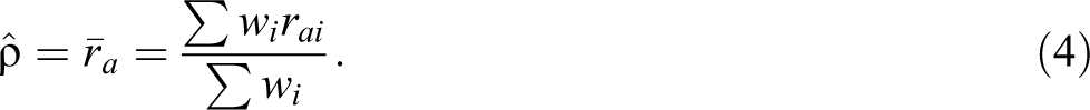
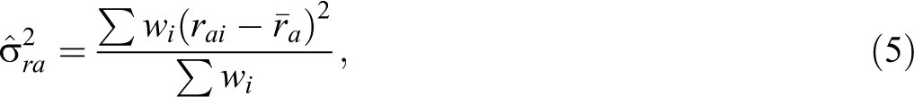
The estimated variance is

{\hat{σ}}_{r a}^{2} = \frac{\sum w_{i} {(r_{a i} - {\bar{r}}_{a})}^{2}}{\sum w_{i}},

and the confidence interval on the mean validity is

C I_{95} = \hat{ρ} \pm 1.96 (\frac{{\hat{σ}}_{r a}}{\sqrt{k}}),

where k is the number of independent effect sizes in the analysis.

Note that the computation of the observed variance does not include the usual adjustment for the bias of the variance (Brannick & Hall, 2001; Field, 2005; Veroniki et al., 2015). Schmidt and Hunter (2015) prefer this estimator because it has a smaller sampling variance. When the number of studies is large (say greater than about 100), the difference between the variance estimated by k vs. k-1 will be trivial, but when the number of effect sizes is small (say 5 or 10) the difference can be large enough to be consequential.

Based on Equation 6, we expect that the 95% confidence intervals will contain the population mean approaching 95% of the time when the number of studies is large (e.g., 100 studies), but the Schmidt-Hunter confidence intervals will be too optimistic (fail to contain the parameter 95% of the time) as the number of studies diminishes. In the simulation, we also computed a version of Schmidt and Hunter in which we multiplied the variance in Equation 5 by k/(k-1) to compensate for the bias in the population estimator to evaluate whether such an adjustment would restore the confidence interval to its nominal level for small k.

The Schmidt-Hunter credibility interval is computed as a function of the random-effects variance component. The observed, weighted mean (unadjusted) correlation is computed by

\bar{r} = \frac{\sum N_{i} r_{i}}{\sum N_{i}} .

The random-effects variance component is computed essentially by subtracting sampling within-studies variance from the total variance. Individual study variance is defined by:

{\hat{σ}}_{a i}^{2} = [\frac{{(1 - {\bar{r}}^{2})}^{2}}{N_{i} - 1}] [\frac{1}{A_{i}^{2}}] .

In the Schmidt-Hunter estimator, sampling error variance is computed by first computing the sample-size weighted mean observed (uncorrected) correlation (Equation 7), then using this value to compute individual study sampling error variance (Equation 8). The weighted average of the within-study variance is computed by:

{\hat{σ}}_{e}^{2} = \frac{\sum w_{i} {\hat{σ}}_{a i}^{2}}{\sum w_{i}},

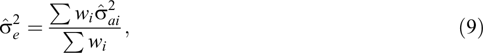
and subtracted from the observed variance (Equation 5) to yield the random-effects variance

{\hat{σ}}_{ρ}^{2} = {\hat{σ}}_{r a}^{2} - {\hat{σ}}_{e}^{2} .

The 80% credibility interval is computed by

C R_{80} = \hat{ρ} \pm 1.28 {\hat{σ}}_{ρ} .

Hedges

So far as we know, Hedges never wrote a paper advocating the analysis that we have labeled “Hedges.” Hedges and Vevea (1998) described a similar approach for uncorrected correlations, and we follow an analysis for artifact corrections suggested by Borenstein et al. (2009). For convenience, we have used Hedges as a label.

Hedges and colleagues (Borenstein et al., 2009; Hedges & Vevea, 1998) label the random-effects variance component tau-squared (τ²); Schmidt and Hunter describe the quantity as the variance of rho and label it Var(ρ); in this article we will refer to the standard deviation of random effects as either τ or σ_ρ and their sample estimates as $\hat{τ}$ and ${\hat{σ}}_{ρ}$ . The Hedges analysis proceeds first by transforming the observed correlations from r to z. In computing the overall mean effect size, Hedges weights each study by the inverse of a variance composed of two pieces (Hedges & Vevea, 1998):

w_{H e d g e s} = {[\frac{1}{N_{i} - 3} + {\hat{τ}}^{2}]}^{- 1} = {[{\hat{σ}}_{z i}^{2} + {\hat{τ}}^{2}]}^{- 1},

where N_i is the study’s sample size (note the Fisher’s r to z has been applied to the correlations; 1/(N_i-3) is the variance of the correlation in z, that is, ${\hat{σ}}_{z i}^{2}$ ). For each observed correlation, there is an associated compound attenuation factor (see the denominator of Equation 2). Weighted regression (where weights are inverse sampling variances) is used to solve for a slope and intercept that relate the attenuation factor to the correlations, that is, the correlations are regressed on the compound attenuation factor (Steel & Kammeyer-Mueller, 2002; Thompson & Higgins, 2002). The resulting equation may be written as:

{z'}_{o} = b_{0} + b_{1} A,

where z′ is the predicted value of the Fisher transformed correlation, the values of b₀ and b₁ are regression coefficients, and A is the compound attenuation factor. Then the predicted value of z and its confidence interval are evaluated at the compound attenuation factor of A = 1.0 (perfect reliability). The predicted value and confidence interval are retranslated from z to r. The calculations for the Hedges approach were completed using the software metafor in R (Viechtbauer, 2010). Random effects variance was estimated by restricted maximum likelihood (REML), as recommended in Viechtbauer (2005).

Unit Weights (Bonett)

For estimating the mean, each study was given equal (unit) weights, and a unit-weighted mean was calculated along with the unit-weighted standard deviation and confidence interval, treating the effect sizes as if they were typical raw data from individual participants in a study (Bonett, 2008). Bonett did not provide estimates for the random-effects variance (his model is fixed-effects, varying coefficients). We used the Schmidt-Hunter equations to estimate the random-effects variance, except that we replaced sample sizes (N_i) with 1s, and used the unit-weighted mean correlation rather than the sample-size-weighted correlation in the computation of the variance. That is, for the random-effects variance, we subtracted sampling variance from observed variance just as in the Schmidt-Hunter equations except for the sample-size weights.

Morris’s Blended Estimator

A recent paper by Morris, Daisley, Wheeler, and Boyer (2015) blended aspects of the Hedges and Schmidt-Hunter approaches to create an estimator that maintains the original metric of r rather than converting to z, but also includes the random-effects variance component in the weights. Because many studies failed to report reliability information, Morris et al. adjusted for unreliability after estimating the mean, confidence interval and credibility interval (that is, the distribution method of correction rather than the individual study method of correction). In the simulation for this article, we adjusted for unreliability in the predictor and the criterion during the analysis rather than afterward (individual study correction); our description of the Morris estimator follows what we did in the simulation. Morris et al. simply reported that they used the approach. They did not evaluate the estimator to see whether it provided better estimates than other available approaches.

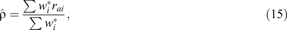
Like Schmidt-Hunter, Morris begins by calculating the disattenuated correlation (adjustment for reliability) using Equation 2. The within-study variances are computed using Equation 8, also as in the Schmidt-Hunter estimator. The disattenuated correlations plus their within-study variances (also disattenuated as shown in Equation 8), were input to metafor, which computed the random-effects variance using REML. The REML estimator of the REVC is intended to compensate for the negative bias in the maximum likelihood estimator when the number of studies is small (Viechtbauer, 2005). In practice, REML cycles between estimates of the mean and the REVC until convergence. The formula for estimating the random-effects variance component is given by Viechtbauer (2005), Equation 18. The random-effects variance was included in the computation of the weights:

w_{i}^{*} = {[{\hat{σ}}_{i}^{2} + {\hat{τ}}^{2}]}^{- 1} .

The weights were then applied to find the mean and its confidence interval:

\hat{ρ} = \frac{\sum w_{i}^{*} r_{a i}}{\sum w_{i}^{*}},

and

C I_{95} = \hat{ρ} \pm 1.96 \frac{1}{\sqrt{\sum w_{i}^{*}}} .

The Morris credibility value was computed by

C R_{80} = \hat{ρ} \pm 1.28 \hat{τ} .

Thus, like the Schmidt-Hunter analysis (but unlike Hedges), the Morris estimator uses the weighted mean r in the calculation of the within-study sampling error. Like the Hedges analysis (but unlike Schmidt-Hunter) the Morris estimator uses the random-effects variance in the weights to estimate the summary (meta-analytic mean) effect. Also unlike the Hedges approach, the artifact adjustments are carried out as an integral part of the analysis rather than as a moderator, and Morris avoids the Fisher z transformation.

Desirable Properties of the Estimators

Meta-analysts have pointed out that the estimators can be shown to provide estimates with good statistical properties when the sample sizes (N_i) and numbers of studies (k) are both large (Borenstein et al., 2009; Hedges & Olkin, 1985; Raudenbush, 2009; Schmidt & Hunter, 2015). Such properties include consistent (asymptotically unbiased) estimates of the population mean and efficient (minimum variance) estimates of the population mean. An additional important property is coverage, that is, confidence intervals that conform to the desired alpha (e.g., a 95% confidence interval will contain the parameter 95% of the time over infinite trials). Unfortunately, there is no guarantee that the large sample properties will apply to small numbers (k) of small sample (N_i) studies, which is a situation that meta-analysts commonly face. In practice, estimates based on small k may be biased (Hedges & Vevea, 1998).

For small k, the Schmidt-Hunter random-effects variance estimate is likely to be too small, resulting in confidence and credibility intervals that are too narrow (Veroniki et al., 2015). On the other hand, the estimate of random effects is likely to have a large sampling variance with small k, and thus the estimate of random-effects variance will be a source of error in the Hedges and Morris estimators because it is included in the weights. The small k meta-analyses are those in which the choice of weights are the most influential, but also where the statistical support is weakest, so the empirical examination of the differences in quality of estimation under such circumstances is important. As the number of studies increases, the choice of weights becomes less important and the statistical justification becomes stronger. We expect to see better performance and better agreement among different estimators as k increases, but it is also important to verify our expectations empirically.

Research Aims

Our research goal was to compare a new estimator (Morris) with four other estimators given realistic underlying distributions, numbers of studies (k) and sample sizes (N_i). We used Monte Carlo simulation with a representative range of underlying parameters and study characteristics to see how each model (Hedges, Schmidt-Hunter [with and without the k correction], Unit, Morris) performed and whether one method might be preferable to another.

Based on the equations used to estimate the mean, we would expect that the Schmidt-Hunter estimator would be less biased on average, especially as the size of the underlying correlation increases and the random-effects variance increases. On the other hand, we would expect that the Hedges estimator would be more efficient (show a smaller root mean square difference between estimate and parameter), especially as the random-effects variance increases.

Method

Overview of the Simulation

We compared five estimators (Hedges, Schmidt-Hunter [with and without the k correction], Unit, Morris) in the quality of estimates of the mean for three dependent variables: (a) bias, (b) root mean square difference between parameter and estimate (RMSE), and (c) coverage of the 95% confidence interval for the mean. We compared the same five estimators in the quality of estimates of the credibility interval for two dependent variables: (a) credibility interval width and (b) absolute difference between sample and population credibility interval bounds. For the credibility intervals, we could in theory apply similar measures to estimators of the random-effects variance. However, the Schmidt-Hunter method does not provide standard errors or confidence intervals for the random-effects variance. Also, the magnitude of the variance is not as easily interpreted as the magnitude of the mean. Therefore, we computed two statistics that appear more directly interpretable to users of meta-analysis.

The first statistic is the width of the credibility interval (upper 80% bound – lower 80% bound), the accuracy of which depends only on the estimate of the random-effects variance. The closer the estimated width is to the population width, the better the estimator.

The second statistic is the absolute value of the difference between the meta-analytic estimate and the population value of the lower and upper bounds of the 80% credibility interval:

D i f f = | (\hat{ρ} - 1.28 {\hat{σ}}_{ρ}) - (ρ - 1.28 σ_{ρ}) | + | (\hat{ρ} + 1.28 {\hat{σ}}_{ρ}) - (ρ + 1.28 σ_{ρ}) | .

A perfect estimator would find the upper and lower bounds exactly, so the difference would be zero. The estimator with the smaller absolute difference is closer on average, and is thus preferred. Note that the accuracy of estimation of the bounds of the credibility interval depends on estimates of both the mean and the random-effects variance. However, the second statistic has the advantage of corresponding more closely to what users of meta-analysis want to know (i.e., the accuracy of credibility value boundary estimates).

The parameters that we manipulated in the simulation were values of the underlying distribution of effect sizes (shape, mean and variance), the number of studies per meta-analysis (k) and the sample sizes (N_i). Each of these is described briefly in turn.

Underlying Distributions

Plausible values

We chose values of mean ρ and σ_ρ that were intended to be representative of values encountered in organizational research (Paterson et al., 2016). Three values of mean ρ were selected: .14, .26, and .42. These values were chosen as the approximate 15th, 50th, and 85th percentiles of the estimated values of ρ in organizational meta-analyses. Three values of σ_ρ were also selected: .08, .13, and .20. These were also based on the similar percentiles of σ_ρ from Paterson et al. (2016). We also added a condition where σ_ρ = 0 to serve as a comparison in which fixed-effects (common effect) was the correct model.

Distribution shape

We chose three different shapes for the underlying distribution of ρ_i. In all three cases, underlying correlations were constrained to fall between -.99 and .99, and were resampled if they fell outside that range. This was accomplished by sampling ten million correlations from a given distribution, and then randomly sampling with replacement from that distribution subject to a constraint that kept the remaining estimates in bound.

Random effects models have generally been developed under the assumption that true effect sizes are normally distributed, which some commentators argue is unrealistic (Bonnet, 2008). In particular, if the underlying distribution is not normal, the bounds of the credibility intervals ( $C R 80 = \hat{ρ} \pm 1.28 {\hat{σ}}_{ρ})$ will be off by an unknown degree. By simulating both normal and nonnormal distributions, we could examine (a) the effect of underlying skew on the estimates of the mean and the credibility interval, and (b) whether the effects were more severe for some estimators than others.

In one condition, the underlying distribution of effect sizes was approximately normal. Strictly speaking, the underlying distribution cannot be normal because the normal has infinite tails, and the correlation is bounded at plus/minus one. In practice, however, if the mean and standard deviation are not extreme, the random number generators very rarely generate values beyond the bounds of the correlation coefficient. For example, in our most extreme distribution, N(.42, .20²), approximately 1 in 1,000 correlations is sampled at a value greater than 1. We considered other distributions, including sampling in z and then transforming to r, but we could not find one that worked as well as the approximate normal with resampling.

In addition to the underlying (approximately) normal distribution, we also constructed underlying distributions with positive and negative skew. The positively and negatively skewed distributions were implemented through the R package “sn” for skewed normal (Azzalini, 2016). For the most extreme values ( $\bar{ρ} = .42$ , σ_ρ = .20, right skew), the distribution was truncated because large values (> .99) were relatively common. Despite this, the accuracy of credibility intervals was defined relative to the 10th and 90th percentiles of the underlying distributions, analogous to the normal.

Artifact Distributions

We simulated reliability of measurement for the independent and dependent variables using the distributions published in Le and Schmidt (2006) and also in Pearlman, Schmidt, and Hunter (1980). Reliability values for the independent variable ranged from 0.50 to 0.90 (M = 0.8, SD = 0.08), and reliability values for the dependent variable ranged from 0.30 to 0.90 (M = 0.6, SD = 0.15). Le and Schmidt (2006) provided graphs illustrating the reliability distributions.

Simulated Study Characteristics

Number of studies

Four values for k were selected to generate the simulated data: 5, 10, 30, and 100. These values of k were selected because the number of studies that published meta-analyses include varies widely. Although 30 to 40 studies is a typical number for overall mean effect size estimates in psychological research, authors often analyze moderators with much smaller numbers of studies (5 or fewer studies are often seen in moderator groupings). Another reason for choosing small numbers of studies is the previously mentioned problem with statistical justification for small k and small N.

Sample sizes

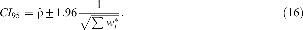
Unlike the other 3 parameters, N was treated as a random variable and a probability distribution was used to generate values. We wanted to simulate the typically skewed distributions of sample size encountered in practice (Sanchez-Meca & Marin-Martinez, 2008). A gamma distribution with shape = 0.57 and scale = 500 was used to generate sample sizes. Because the gamma distribution can generate values that are not integers, all noninteger values were rounded up to the nearest whole number. Only integer values of 30 or greater were allowed because correlations based on smaller sample sizes are rare in organizational research. One million sample values were generated from this distribution, and sampling with replacement was used to keep only values of 30 or greater. For the resulting sample size distribution, the mean was 390, the median was 223, the standard deviation was 465, and skew was 2.5. Figure 1 illustrates the distribution of sample sizes (there are larger samples than what are displayed in the figure the maximum was approximately N = 5,800). This distribution is intended to represent sample sizes that organizational researchers are likely to encounter in the research literature (see Table 2 in Paterson et al., 2016).

Figure 1.

Distribution of Sample Sizes.

Special comparisons

For certain cells of the design (all conditions where $\bar{ρ} = .26, σ_{ρ}^{2} = 0; \bar{ρ} = .26, σ_{ρ} = .20$ ), we ran a comparison using a uniform distribution of sample sizes ranging from 70 to 150, which was the distribution reported in Le and Schmidt (2006). As a second special comparison, we simulated data ( $\bar{ρ} = .26, σ_{ρ} = .13$ ) based on a sample sizes from a convenience sample of three published meta-analyses to compare to the results from using the gamma distribution. The purpose of the special comparisons was (a) to isolate the effect of sample size distribution (skewed, large sample vs. uniform, small sample) and (b) to check whether the results of the simulation could apply to real organizational science meta-analyses. We also used data from three published meta-analysis as examples to estimate the mean and 95% confidence interval to show empirically the effects of choice of estimator on a small sample of published meta-analyses.

Procedure

The software package R was used for the simulation. Code used in the simulation may be downloaded at https://github.com/MichaelBrannick/InPublications. Each possible combination of values for the ρ distribution (left-skewed, normal, right-skewed), ρ, σ_ρ, and k, was simulated for a total of 120 different conditions (including the 12 conditions in which there was no random-effects variance).

The simulation began by setting up a population correlation matrix that included variables for both true scores and observed scores. The population matrix allowed for the effects of attenuation for reliability and for computing both observed correlations and observed reliabilities (see Le & Schmidt, 2006, Figure 1, where variables Tx and Ty represent true scores for predictor and criterion, and X and Y represent observed scores for predictor and criterion).

The parameters of the simulation were used to associate numbers with the population matrix. For example, one condition in our simulation was underlying approximately normal, $\bar{ρ}$ = .26, σ_ρ = .13, k = 10. For each of the 10 studies, a value of ρ_i would be drawn from the approximately normal distribution with mean equal to .26 and standard deviation equal to .13. That value would be inserted as the correlation between true scores Tx and Ty in the population matrix. Reliabilities would be randomly sampled from the predictor and criterion reliability distributions. The reliabilities were used to set the correlations between true and observed scores in the population (that is, the correlations between Tx and X and between Ty and Y). The population observed correlation between attenuated observed scores was also computed (the correlation between X and Y is the population attenuated correlation). At this point we had population values ρ _(Tx,X), ρ _(Ty,Y), and ρ _(X,Y). Because (in this instance) k = 10, there would be 10 such matrices, one for each local population. The goal of the meta-analysis is to estimate ρ _(Tx,Ty), the underlying correlation between true scores.

Next, for each of the 10 matrices, a sample size, N_{i ,} was independently sampled from the gamma distribution, and N_i raw observations (observed scores) were drawn from a multivariate normal distribution with the given population correlation matrix. Observed correlations were computed for observed scores on X and Y (observed predictor and criterion) and were also computed between Tx and X (predictor reliability) and Ty and Y (criterion reliability). (Technically, the population correlations between the true and observed scores in our simulations are the square roots of the reliabilities.) At this point, we had 10 observed correlations and reliability estimates, each computed on an independent sample.

Finally, the 10 observed correlations and reliability estimates were meta-analyzed, resulting in an overall mean effect size, confidence interval and credibility interval for each of our meta-analysis methods. We determined the relations between the estimated mean and the population parameter (bias and RMSE), the proportion of times the confidence interval contained the population value (coverage), and examined the quality of the credibility interval (credibility interval width and difference between estimated and population bounds). This process was computed 10,000 times per condition.

Results

Mean Correlations

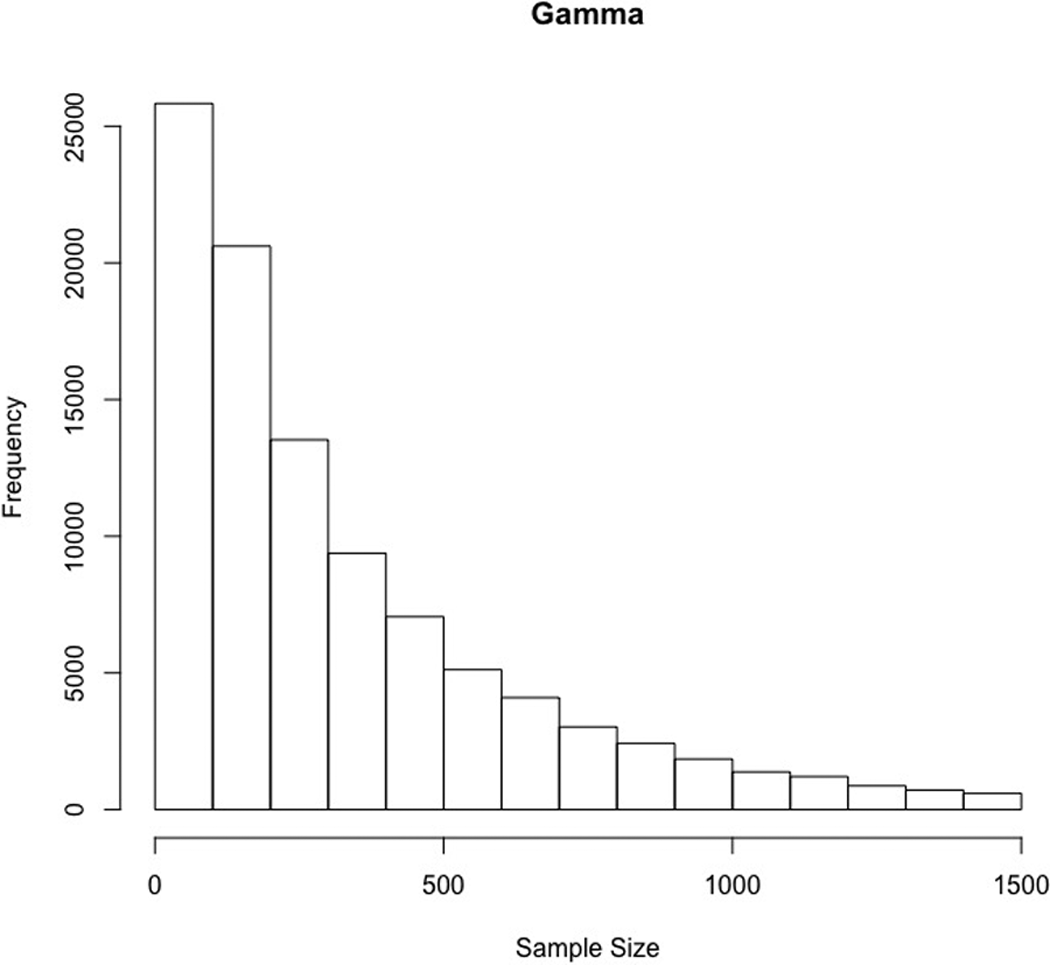
Tables 1 to 3 present the results of average bias, RMSE, and coverage across the Hedges, Schmidt-Hunter, Morris, and Unit estimators as a function of the underlying mean correlation ( $\bar{ρ}$ ), standard deviation of the underlying distribution (σ_ρ), and number of samples (k). The results of bias, RMSE, and coverage of the 95% confidence interval for the mean across left and right skewed $\bar{ρ}$ distributions are not presented because the magnitude and pattern of results was similar to the normal distribution. Interested readers are directed to the online supplementary material to find those results. As shown in Table 1, the average bias in the estimate of the overall mean effect size across conditions of all estimators except Hedges was negligible. Hedges displayed a negative bias when number of studies was small (k = 5). However, Hedges became more positively biased as number of studies and σ_ρ increased. Hedges also became more positively biased as the underlying correlation $\bar{ρ}$ increased in conditions where random-effects variance was very large (σ_ρ = .2). However, the bias associated with Hedges across all conditions was modest overall.

Table 1.

Mean Bias of Estimates of the Overall Effect Size as a Function of Population Mean, Standard Deviation, and Number of Studies.

	$\bar{ρ} = .14$				$\bar{ρ} = .26$				$\bar{ρ} = .42$
Method	k = 5	k = 10	k = 30	k = 100	k = 5	k = 10	k = 30	k = 100	k = 5	k = 10	k = 30	k = 100
	σ_ρ = .00
Hedges	.00	.00	.00	.00	.00	.00	.00	.00	–.01	.00	.00	.00
S-H	.00	.00	.00	.00	.00	.00	.00	.00	.00	.00	.00	.00
Morris	.00	.00	.00	.00	.00	.00	.00	.00	.00	.00	.00	.00
Unit	.00	.00	.00	.00	.00	.00	.00	.00	.00	.00	.00	.00
	σ_ρ = .08
Hedges	.00	.00	.00	.00	.00	.00	.01	.00	–.01	.00	.00	.00
S-H	.00	.00	.00	.00	.00	.00	.00	.00	.00	.00	.00	.00
Morris	.00	.00	.00	.00	.00	.00	.00	.00	.00	.00	.00	.00
Unit	.00	.00	.00	.00	.00	.00	.00	.00	.00	.00	.00	.00
	σ_ρ = .13
Hedges	.00	.00	.01	.00	–.01	.00	.01	.01	–.01	.00	.01	.01
S-H	.00	.00	.00	.00	.00	.00	.00	.00	.00	.00	.00	.00
Morris	.00	.00	.00	.00	.00	.00	.00	.00	.00	.00	.00	.00
Unit	.00	.00	.00	.00	.00	.00	.00	.00	.00	.00	.00	.00
	σ_ρ = .20
Hedges	.00	.00	.01	.01	–.01	.00	.01	.01	–.03	.00	.01	.02
S-H	.00	.00	.00	.00	.00	.00	.00	.00	.00	.00	.00	.00
Morris	.00	.00	.00	.00	.00	.00	.00	.00	.00	.00	.00	.00
Unit	.00	.00	.00	.00	.00	.00	.00	.00	.00	.00	.00	.00

Note: S-H = Schmidt-Hunter. Schmidt-Hunter estimator with the k correction is omitted because its bias is identical to the Schmidt-Hunter estimator.

Table 2.

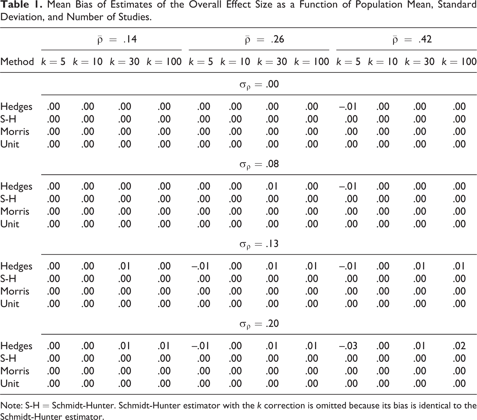
Mean Root Mean Square Error as a Function of Population Mean, Standard Deviation, and Number of Studies.

	$\bar{ρ} = .14$				$\bar{ρ} = .26$				$\bar{ρ} = .42$
Method	k = 5	k = 10	k = 30	k = 100	k = 5	k = 10	k = 30	k = 100	k = 5	k = 10	k = 30	k = 100
	σ_ρ = .00
Hedges	.15	.08	.04	.02	.14	.07	.03	.02	.12	.06	.03	.02
S-H	.04	.03	.01	.01	.04	.03	.01	.01	.03	.02	.01	.01
Morris	.04	.03	.01	.01	.04	.03	.01	.01	.04	.02	.01	.01
Unit	.06	.04	.02	.01	.06	.04	.02	.01	.05	.04	.02	.01
	σ_ρ = .08
Hedges	.19	.11	.06	.03	.19	.11	.05	.03	.17	.10	.05	.03
S-H	.06	.04	.03	.01	.06	.04	.03	.01	.06	.04	.03	.01
Morris	.06	.04	.02	.01	.06	.04	.02	.01	.06	.04	.02	.01
Unit	.07	.05	.03	.02	.07	.05	.03	.02	.06	.05	.03	.02
	σ_ρ = .13
Hedges	.24	.15	.08	.04	.24	.14	.07	.04	.22	.13	.07	.04
S-H	.09	.06	.04	.02	.09	.06	.04	.02	.08	.06	.04	.02
Morris	.08	.05	.03	.02	.08	.05	.03	.02	.07	.05	.03	.02
Unit	.08	.06	.03	.02	.08	.06	.03	.02	.08	.06	.03	.02
	σ_ρ = .20
Hedges	.31	.20	.11	.06	.30	.19	.10	.06	.29	.18	.10	.05
S-H	.12	.09	.06	.03	.13	.09	.06	.03	.12	.09	.06	.03
Morris	.10	.07	.04	.02	.10	.07	.04	.02	.10	.07	.04	.02
Unit	.11	.08	.04	.02	.11	.08	.04	.02	.10	.07	.04	.02

Note: S-H = Schmidt-Hunter. RMSE = root mean square difference between estimate and parameter. Schmidt-Hunter estimators with the k correction is omitted because its RMSE is identical to the Schmidt-Hunter estimator.

Table 3.

Mean Coverage of the 95% Confidence Interval for the Mean as a Function of Population Mean, Standard Deviation, and Number of Studies.

	$\bar{ρ} = .14$				$\bar{ρ} = .26$				$\bar{ρ} = .42$
Method	k = 5	k = 10	k = 30	k = 100	k = 5	k = 10	k = 30	k = 100	k = 5	k = 10	k = 30	k = 100
	σ_ρ = .00
Hedges	.97	.96	.95	.95	.97 (.96)	.96 (.96)	.96 (.96)	.96 (.95)	.97	.97	.96	.96
S-H	.85	.91	.94	.95	.85 (.84)	.90 (.90)	.93 (.93)	.95 (.95)	.85	.91	.94	.95
S-H-k	.88	.92	.94	.95	.88 (.88)	.92 (.92)	.94 (.94)	.95 (.95)	.88	.92	.94	.95
Morris	.97	.96	.96	.96	.97 (.91)	.96 (.93)	.96 (.94)	.96 (.95)	.97	.96	.97	.96
Unit	.89	.93	.95	.95	.90 (.88)	.93 (.92)	.94 (.94)	.95 (.95)	.90	.93	.94	.95
	σ_ρ = .08
Hedges	.89	.90	.93	.94	.89	.90	.93	.93	.89	.90	.92	.93
S-H	.77	.83	.85	.86	.77	.82	.85	.86	.76	.82	.84	.85
S-H-k	.81	.85	.86	.87	.81	.84	.85	.86	.81	.84	.85	.86
Morris	.89	.91	.93	.95	.89	.90	.93	.95	.89	.90	.93	.95
Unit	.89	.92	.94	.95	.88	.92	.94	.95	.88	.92	.94	.95
	σ_ρ = .13
Hedges	.86	.89	.93	.93	.85	.89	.93	.93	.85	.89	.93	.92
S-H	.73	.79	.82	.83	.73	.79	.82	.83	.72	.79	.81	.82
S-H-k	.78	.81	.83	.83	.78	.81	.82	.83	.77	.81	.82	.82
Morris	.86	.90	.94	.95	.86	.90	.94	.95	.86	.90	.94	.95
Unit	.88	.92	.94	.95	.88	.92	.94	.95	.88	.92	.94	.95
	σ_ρ = .20
Hedges	.83	.90	.93	.93	.84 (.87)	.89 (.91)	.92 (.92)	.92 (.92)	.85	.89	.92	.91
S-H	.71	.78	.80	.81	.71 (.83)	.77 (.90)	.81 (.92)	.81 (.94)	.72	.77	.81	.81
S-H-k	.76	.80	.81	.81	.75 (.87)	.79 (.91)	.81 (.93)	.81 (.94)	.76	.80	.81	.81
Morris	.86	.91	.94	.95	.86 (.88)	.91 (.92)	.94 (.94)	.95 (.95)	.86	.91	.94	.95
Unit	.88	.92	.94	.95	.88 (.88)	.92 (.92)	.94 (.94)	.95 (.95)	.88	.92	.94	.95

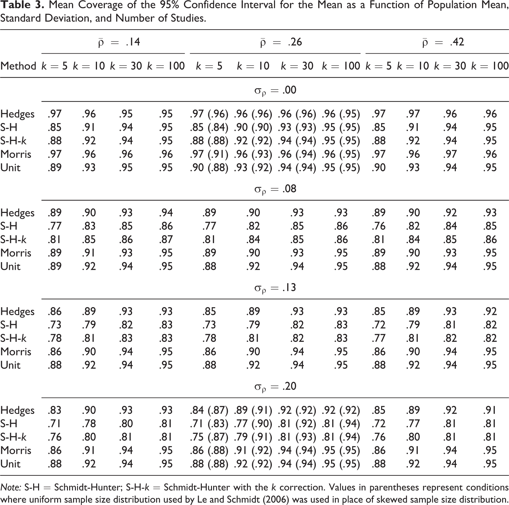
Note: S-H = Schmidt-Hunter; S-H-k = Schmidt-Hunter with the k correction. Values in parentheses represent conditions where uniform sample size distribution used by Le and Schmidt (2006) was used in place of skewed sample size distribution.

Table 2 presents the results regarding the statistical efficiency (RMSE) of each method. Contrary to our expectations, the Hedges estimator never had smaller RMSE compared to Schmidt-Hunter, even as the random-effects variance (σ_ρ) increased. In fact, Hedges consistently displayed the largest RMSE across any condition, with markedly larger RMSE values when the number of studies was smaller (k between 5 and 10). Unlike other estimators, Hedges also displayed smaller RMSEs as the underlying mean correlation increased. Such a result appears to be due to the use of regression to model the artifacts (there is error of estimation in the slope). All estimators displayed reasonably small RMSE values when the number of studies was large (k = 100). However, the Morris and Unit estimators displayed noticeably smaller RMSE values than Schmidt-Hunter when the number of studies was smaller (k ≤ 30) and the random effects variance was large (σ_ρ = .20). Across all conditions, Morris displayed RMSE values that were either the smallest or similar in magnitude compared to Schmidt-Hunter and Unit.

Table 3 presents the results for coverage of the 95% confidence interval for the mean for each estimator across all conditions. The value of $\bar{ρ}$ had essentially no effect on coverage for any estimator. The Schmidt-Hunter estimator and its k-corrected version consistently displayed levels of coverage below the nominal .95 value across all conditions in which there was random-effects variance. Only when no random-effect variance was present and the number of studies was large (k ≥ 30) was the Schmidt-Hunter level of coverage similar to Hedges, Morris, and Unit. The Hedges and Morris estimators both displayed higher coverage than Unit when no random variance was present. However, the Unit estimator generally displayed the highest coverage when random-effects variance increased (σ_ρ ≥ .08). The Morris estimator also displayed high levels of coverage when the number of studies was moderately large (k ≥ 30). Figure 2 summarizes the coverage results across all skewed-sample conditions in the study using boxplots to show the distributions.

Figure 2.

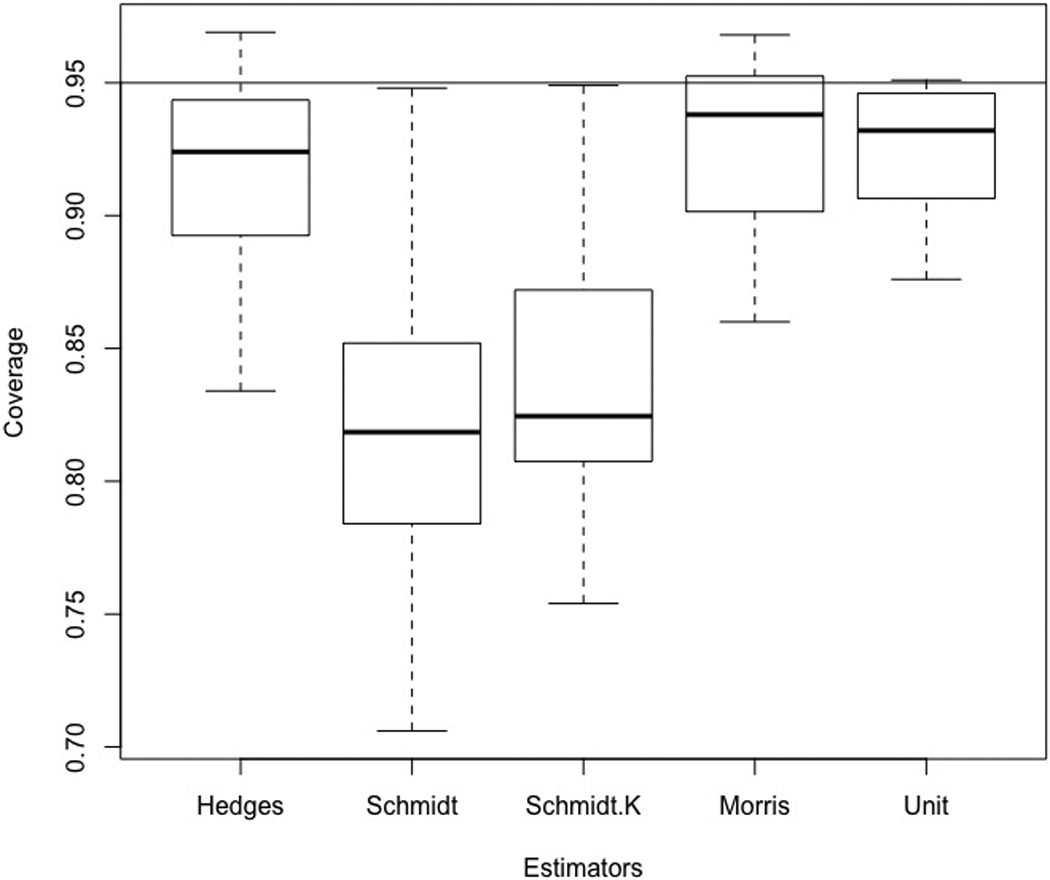
Boxplots of Coverage Estimates.

Table 3 also shows the results for the uniform distribution of sample sizes (bounded by the interval 70 to 150). Of particular interest is the results for the Schmidt-Hunter estimators, which show coverage approaching nominal levels as k increases, even when the random-effects variance is large, provided that the sample size distribution is uniform.

Credibility Intervals

Tables 4 and 5 display the mean absolute difference of the lower and upper bounds of the credibility interval and the credibility interval width for each estimator across all conditions. All estimators displayed larger absolute differences when the underlying correlation distribution was skewed. However, the pattern of results was similar to those seen with the normal distribution. For ease of interpretation, only the results for the normal distribution conditions are presented here. Interested readers are directed to the supplementary material to find the results for underlying skewed distributions. As shown in Table 4, the Morris estimator had the smaller absolute difference across most conditions. The only exceptions were when sample size was small (k = 5) and when there was a small amount of random effect variance present (σ_ρ ≤ .08). In those cases, Schmidt-Hunter displayed the smallest absolute differences when no random effects variance was present (σ_ρ = 0); the Schmidt-Hunter and its k-corrected version displayed the smallest absolute difference when random effects variance was small (σ_ρ = .08). The Unit estimator also outperformed the Schmidt-Hunter estimators when random-effects variance became very large (σ_ρ = .20). Figure 3 shows boxplots illustrating the results of the difference between estimated credibility boundaries and actual boundaries across all skewed-sample conditions.

Table 4.

Mean Credibility Endpoint Difference as a Function of Population Mean, Standard Deviation, and Number of Studies.

	$\bar{ρ} = .14$				$\bar{ρ} = .26$				$\bar{ρ} = .42$
Method	k = 5	k = 10	k = 30	k = 100	k = 5	k = 10	k = 30	k = 100	k = 5	k = 10	k = 30	k = 100
	σ_ρ = .00
Hedges	.56	.32	.16	.08	.53	.30	.15	.08	.47	.26	.13	.07
S-H	.08	.07	.05	.03	.08	.06	.04	.03	.07	.05	.04	.02
S-H-k	.10	.08	.05	.03	.10	.07	.05	.03	.09	.06	.04	.02
Morris	.10	.07	.05	.03	.10	.07	.04	.03	.09	.06	.04	.02
Unit	.15	.13	.09	.07	.14	.12	.08	.05	.12	.09	.06	.03
	σ_ρ = .08
Hedges	.50	.28	.13	.06	.47	.26	.12	.06	.43	.23	.10	.05
S-H	.16	.12	.07	.04	.16	.12	.07	.03	.16	.12	.07	.03
S-H-k	.16	.11	.07	.03	.15	.11	.06	.03	.15	.11	.06	.03
Morris	.16	.12	.06	.03	.16	.11	.06	.03	.15	.11	.06	.03
Unit	.19	.16	.12	.07	.19	.16	.12	.08	.19	.16	.13	.11
	σ_ρ = .13
Hedges	.55	.33	.16	.08	.53	.32	.15	.07	.49	.28	.13	.07
S-H	.22	.15	.09	.05	.22	.15	.09	.05	.21	.15	.09	.05
S-H-k	.21	.15	.08	.05	.21	.15	.08	.05	.20	.14	.08	.05
Morris	.20	.14	.07	.04	.20	.14	.07	.04	.20	.13	.07	.04
Unit	.23	.17	.10	.06	.23	.17	.11	.06	.23	.18	.11	.07
	σ_ρ = .20
Hedges	.63	.40	.20	.10	.61	.39	.19	.10	.59	.35	.17	.09
S-H	.30	.21	.12	.07	.30	.21	.12	.07	.29	.21	.12	.07
S-H-k	.28	.20	.12	.07	.29	.20	.12	.07	.28	.20	.12	.07
Morris	.26	.17	.10	.05	.26	.17	.10	.05	.25	.17	.09	.05
Unit	.28	.19	.11	.06	.28	.19	.11	.06	.28	.20	.11	.07

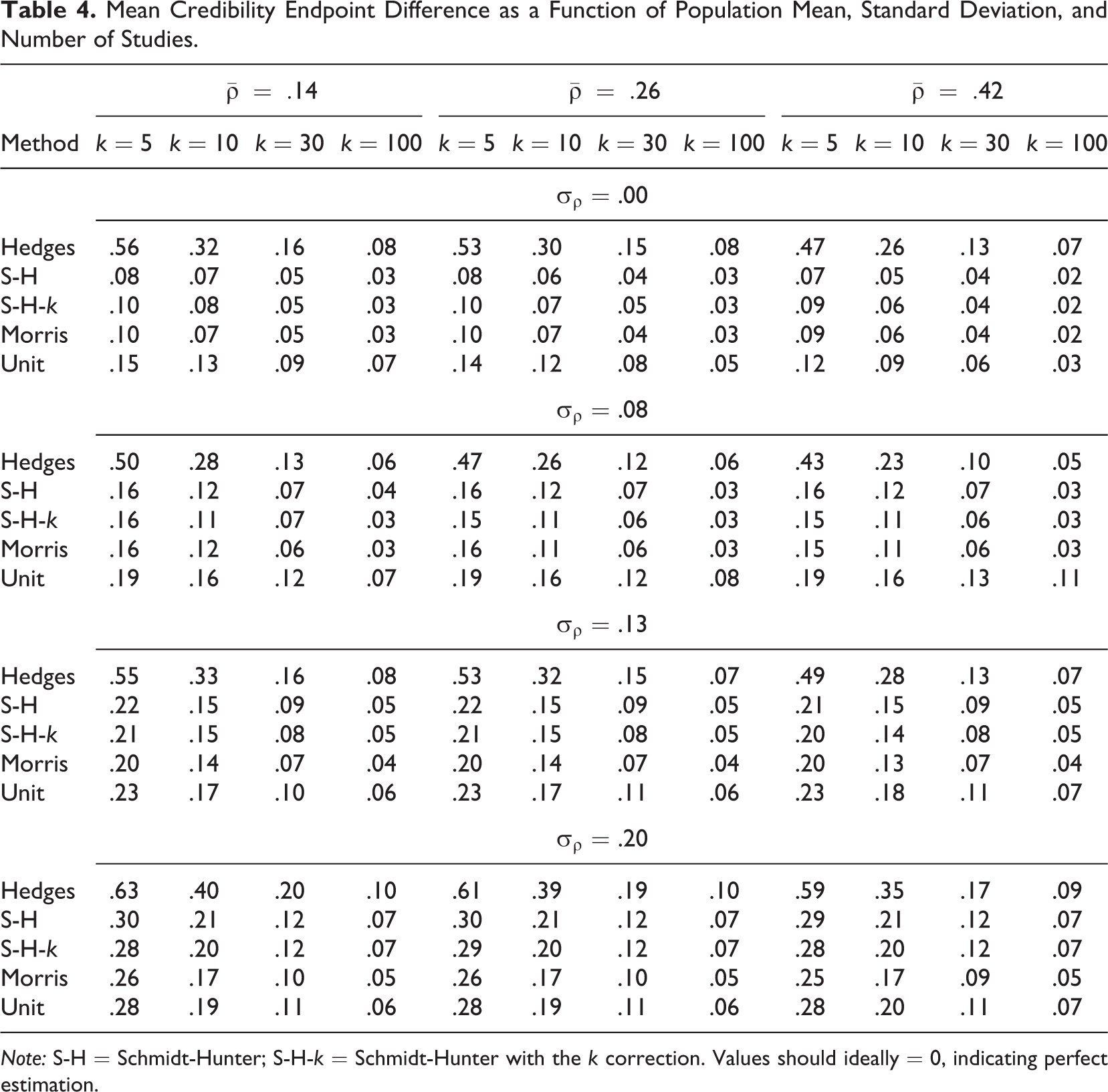
Note: S-H = Schmidt-Hunter; S-H-k = Schmidt-Hunter with the k correction. Values should ideally = 0, indicating perfect estimation.

Table 5.

Mean Credibility Interval Width.

	$\bar{ρ} = .14$				$\bar{ρ} = .26$				$\bar{ρ} = .42$
Method	k = 5	k = 10	k = 30	k = 100	k = 5	k = 10	k = 30	k = 100	k = 5	k = 10	k = 30	k = 100
	σ_ρ = .00 (w = 0)
Hedges	.56	.31	.15	.08	.53	.30	.15	.08	.47	.26	.13	.06
S-H	.04	.04	.03	.03	.04	.04	.03	.02	.03	.03	.02	.01
S-H-k	.06	.05	.04	.03	.06	.05	.03	.02	.05	.04	.02	.01
Morris	.07	.05	.03	.02	.06	.05	.03	.02	.05	.04	.02	.01
Unit	.10	.09	.07	.05	.09	.08	.06	.04	.07	.05	.03	.02
	σ_ρ = .08 (w = .205)
Hedges	.66	.43	.29	.24	.63	.41	.28	.23	.58	.37	.26	.21
S-H	.11	.14	.18	.20	.11	.14	.18	.20	.11	.14	.18	.19
S-H-k	.15	.16	.19	.20	.15	.16	.19	.20	.14	.16	.18	.19
Morris	.16	.18	.19	.20	.16	.17	.19	.20	.16	.17	.19	.20
Unit	.17	.17	.17	.18	.16	.15	.15	.16	.13	.13	.11	.11
	σ_ρ = .13 (w = .333)
Hedges	.77	.58	.44	.38	.75	.56	.42	.37	.70	.52	.39	.34
S-H	.20	.26	.31	.32	.20	.26	.31	.32	.20	.26	.31	.32
S-H-k	.25	.29	.32	.33	.25	.29	.32	.33	.25	.28	.31	.32
Morris	.28	.30	.32	.33	.27	.30	.32	.33	.27	.30	.32	.32
Unit	.27	.28	.30	.32	.26	.27	.29	.31	.24	.25	.27	.28
	σ_ρ = .20 (w = .512)
Hedges	.95	.79	.64	.57	.93	.77	.62	.56	.91	.73	.58	.52
S-H	.34	.42	.48	.50	.34	.42	.48	.50	.35	.42	.48	.50
S-H-k	.40	.45	.49	.50	.40	.45	.49	.50	.40	.45	.49	.50
Morris	.45	.48	.50	.51	.45	.48	.50	.51	.45	.48	.50	.50
Unit	.43	.47	.49	.50	.43	.46	.49	.49	.41	.44	.47	.47

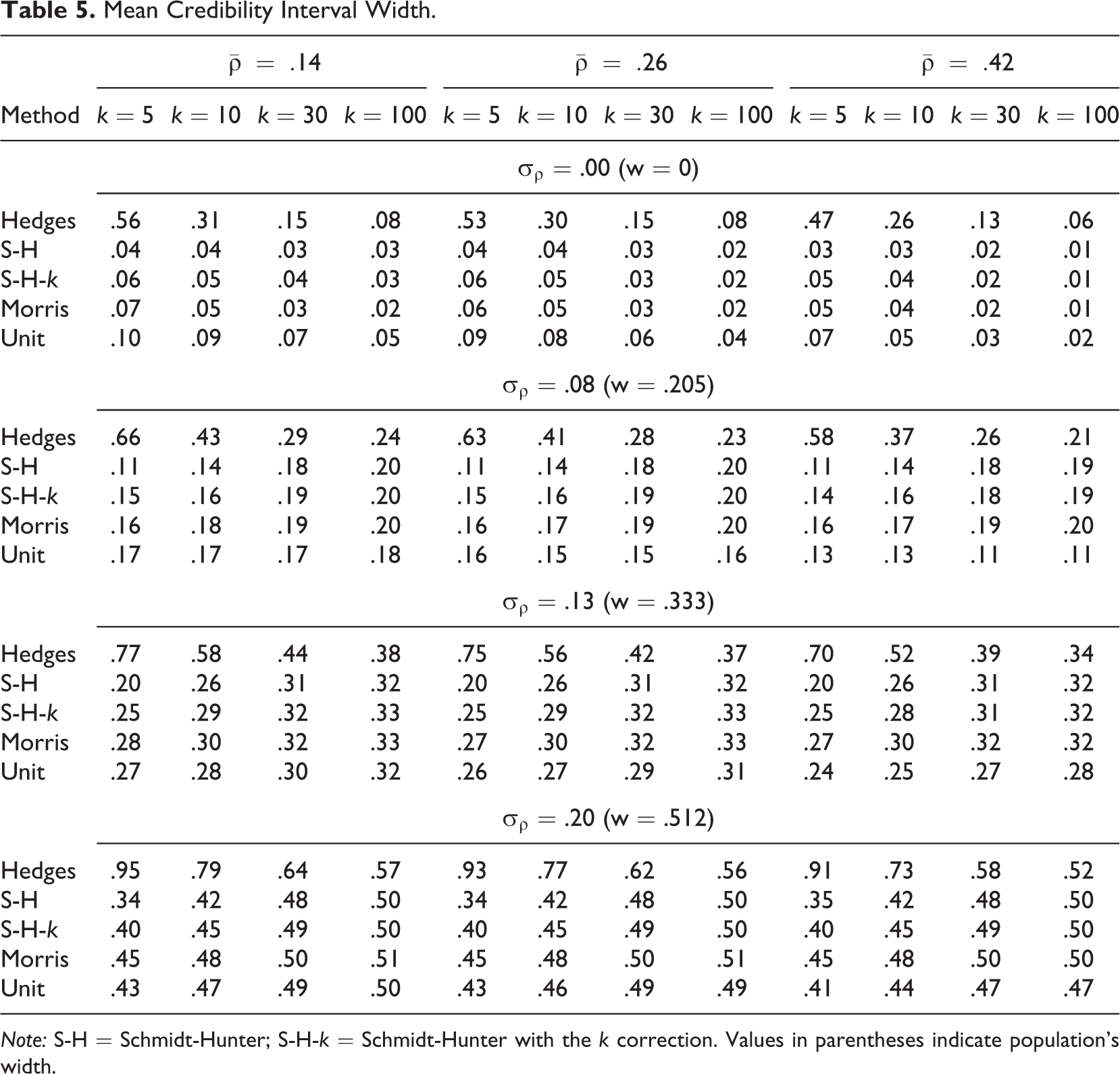
Note: S-H = Schmidt-Hunter; S-H-k = Schmidt-Hunter with the k correction. Values in parentheses indicate population’s width.

Figure 3.

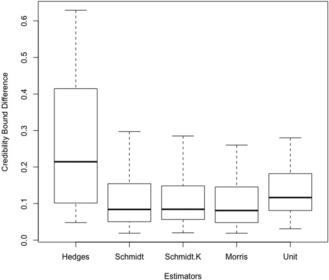
Boxplots of Differences Between Credibility Bounds Estimates and Parameters.

As shown in Table 5, the Morris estimator provided the closest credibility interval width to the nominal width (the population’s width) in most conditions. The Hedges estimator displayed credibility interval widths furthest from the nominal width across all conditions. The Morris estimator outperformed both Schmidt-Hunter estimators when random-effects variance was present (σ_ρ ≥ .08). When the number of studies was large (k = 100), Morris and Schmidt-Hunter estimated similar widths. The Morris estimator also outperformed Unit across most conditions except when random-effects variance was small (σ_ρ = .08) and number of studies was very small (k = 5). Unlike the other estimators, Unit displayed smaller widths as the underlying mean correlation increased.

Table 6 shows the examples of application to real data, first through coverage estimates obtained through simulated data and second through the application of the estimators to the published data. Coverage estimates showed the same pattern as the simulated weights distributions; Schmidt-Hunter coverage was less than the other methods. Estimates of the mean across methods differed by as little as .01 and as much a .07. Confidence intervals across methods showed varying degrees of overlap from near complete overlap to essentially nonoverlapping.

Table 6.

Published Study Distributions Mean Coverage of the 95% Confidence Interval for the Mean Plus Estimates of the Overall Mean Effect Size and Confidence Interval for Original Studies.

	McEvoy (k = 24)				Morris (k = 46)				Rabl (k = 156)
Method	Cov	M	LB	UB	Cov	M	LB	UB	Cov	M	LB	UB
Hedges	.94	-.20	-.28	-.11	.92	.28	.22	.34	.93	.29	.26	.32
S-H	.84	-.22	-.28	-.15	.89	.24	.19	.30	.79	.22	.20	.25
S-H-k	.84	-.22	-.28	-.15	.90	.24	.19	.30	.79	.22	.20	.25
Morris	.92	-.19	-.27	-.11	.94	.27	.22	.32	.95	.28	.25	.31
Unit	.94	-.19	-.26	-.11	.94	.30	.24	.35	.95	.28	.25	.31

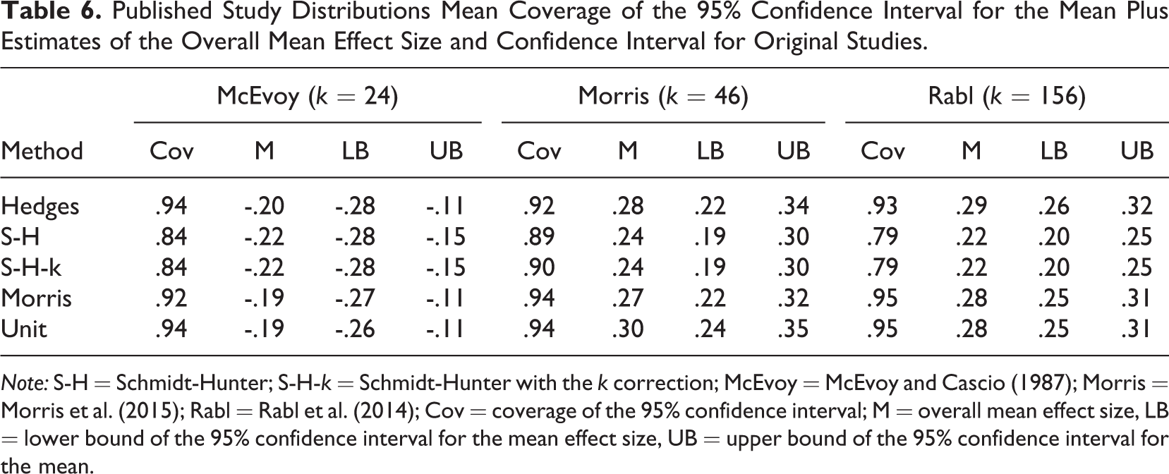
Note: S-H = Schmidt-Hunter; S-H-k = Schmidt-Hunter with the k correction; McEvoy = McEvoy and Cascio (1987); Morris = Morris et al. (2015); Rabl = Rabl et al. (2014); Cov = coverage of the 95% confidence interval; M = overall mean effect size, LB = lower bound of the 95% confidence interval for the mean effect size, UB = upper bound of the 95% confidence interval for the mean.

Discussion

Because meta-analytic results tend to be regarded as dependable and conclusions based on them are highly cited, it is important to use meta-analytic methods that provide the most accurate results. The main purpose of this study was to compare the performance of a newly developed meta-analytic estimator (Morris et al., 2015) with a set of reference estimators (Unit, Hedges, Schmidt-Hunter). The results of this simulation suggest that the Morris method is a viable estimator of the overall meta-analytic mean and credibility interval. Regarding the mean, or overall summary estimate, the Morris approach showed lower levels of bias than the Hedges method and better coverage of the 95% confidence interval of the mean than the Schmidt-Hunter method. The Morris estimator showed RMSE values as good as or better than the reference estimators.

There are two key reasons for the differences in performance among the estimators. First is the size of the population random-effects variance. As that variance increases, the statistically optimal weights become closer to unit weights (Hedges & Olkin, 1985; Hedges & Vevea, 1998). Thus, when the random-effects variance is small, the Schmidt-Hunter weights fare relatively well, and when the random-effects variance is large, Unit weights fare relatively well. Unlike Schmidt-Hunter and Unit, both the Hedges and Morris approaches estimate the REVC and use it in calculating the overall mean effect size. Thus, Hedges and Morris have the advantage of flexibility in covering different magnitudes of the REVC but the disadvantage of having to estimate the REVC.

The second key reason for the difference in performance among the estimators is the distribution of sample sizes. If the sample size distribution is skewed and there is a large REVC, a very large sample size may by chance correspond to a population value quite discrepant from the overall mean ( $\bar{ρ}$ ). Such an occurrence will likely produce a correlation between sample size and effect size in that meta-analysis, even if the correlation between the two is zero in the population. The obtained correlation between sample size and effect size will be a greater problem for Schmidt-Hunter estimator than for the others. We expand on each of these points during the discussion of the results corresponding to each estimator.

Schmidt-Hunter Estimator

The Schmidt-Hunter estimator has a long history of successful application in applied psychology and organizational research. As Schmidt and Hunter (2015) noted, the estimator’s weights work well unless there is a correlation between the sample size and the effect size. In our simulation, the sample size and effect size were uncorrelated in the population of studies, but as we mentioned previously, the combination of large random-effects variance and skewed sample size results in correlations between effect size and sample size for some meta-analyses. In such circumstances, large-sample effect sizes exert undue influence on the overall estimate, moving the estimated mean away from its population value and resulting in coverage rates that are less than their nominal value, that is, confidence intervals will fail to contain the population mean effect size more often than they should. The smaller the number of studies, the greater the instances of large correlations between effect size and sample size due solely to chance.

The Schmidt-Hunter estimator of between-study variance is known to be biased (Brannick & Hall, 2001; Veroniki et al., 2015), so we incorporated a k corrected version of this estimator. As expected, the k correction resulted in improved coverage and improved credibility interval width with small numbers of studies. However, the k correction failed to yield coverage at its nominal rate given skewed sample size distributions. Nor did it result in average credibility intervals equal to their theoretical values.

Given sufficient numbers of studies, the Schmidt-Hunter estimator of the overall mean effect size works well in terms of bias, efficiency and coverage when the random-effects variance is small and the sample sizes are not too discrepant. The Schmidt-Hunter weights effectively assume no random-effects variance, and so are well suited to conditions where there is none.

Regarding sample sizes, some of the studies evaluating the Schmidt-Hunter estimator have chosen a restricted sample size distribution. For example, the Le and Schmidt (2006) sample sizes were “randomly selected between 70 and 150” (p. 423) and Law, Schmidt, and Hunter (1994) chose sample sizes between 30 and 150. Other studies have treated sample size as a fixed factor, such that all the studies within a given condition contained identical sample sizes (Fife, Hunter, & Mendoza, 2016; Fife, Mendoza, & Terry, 2013; Law, 1995; Le, Oh, Schmidt, & Wooldridge, 2016). Note that having equal sample sizes is tantamount to using unit weights for calculating the mean effect size. The impact of the distribution of sample sizes cannot be evaluated when the sample size is constant.

When there is random-effects variance, a skewed distribution of sample sizes is likely to prove troublesome to the Schmidt-Hunter weighting scheme. To illustrate this point, we ran a comparison condition in which we held constant everything but the sample size distribution. The comparison sample sizes were sampled from a uniform distribution with a relatively narrow range (70 to 150), as in Le and Schmidt (2006). With the uniform distribution of sample sizes, there was essentially no difference in coverage between the conditions with no random-effects variance and large random-effects variance for the Schmidt-Hunter estimates (see Table 3). Coverage rose as function of the number of studies, and the k correction was helpful for small numbers of studies. For example, when the number of studies was 100, the coverage for the skewed sample sizes was .81, but for restricted sample sizes (uniform between 70 and 150) it was .94.

Hedges Estimator

Consistent with previous studies (Brannick et al., 2011; Field, 2001, 2005; Hafdahl & Williams, 2009; Hall & Brannick, 2002), current results demonstrated greater bias with the Hedges estimator than the Schmidt-Hunter estimator. The bias problem with the Hedges approach appears to be the r to z transformation (Schmidt & Hunter, 2015). Bias for Hedges increases as the parameters $\bar{ρ}$ and σ_ρ increase. Because the simulation will produce very large values of r, and these will become much larger with the transformation, the mean becomes increasingly biased as more such cases occur. Both Hafdahl and Williams (2009) and Law (1995) suggested that other methods of retranslation of z to r may result in more comparable estimates between Hedges and Schmidt-Hunter. Thus, the small difference in bias may ultimately prove an unfair comparison. The Hedges estimator also had poorer coverage when both $\bar{ρ}$ and σ_ρ were large, presumably due to bias in the estimate of the mean.

Results of modelling unreliability as a moderator suggest that this approach (Borenstein et al., 2009) can produce consistent estimates of the underlying disattenuated correlation; bias for this estimator was roughly equivalent to the other estimators. However, the weighted regression model requires large numbers of studies before its efficiency approaches that of the other estimators. Even with 100 studies, the RMSE for Hedges was often twice that for the other estimators. Such a result is unsurprising because of sampling error in the slope relating reliability to effect size. In some areas of research, corrections for reliability are not employed, so the relative efficiency in such situations would be much improved in comparison to the current study. To the best of our knowledge, this study is the first to compare Hedges (using weighted regression) and Schmidt-Hunter estimators when adjusting for reliability of measurement.

Bonett Estimator (Unit Weights)

Consistent with Brannick et al. (2011), the unit weighting scheme proposed by Bonett worked well in terms of bias. As one would expect, the RMSE was larger for the Unit estimator than for Schmidt-Hunter estimator when the number of studies was small, but the difference diminished as the number of studies increased.

Unit weights also tended to work well in terms of coverage of the 95% confidence interval for the mean except when the number of studies was small and the random-effects variance was large. Such a result is to be expected because a small sample of studies may not be representative of the parent population when the random-effects variance is large. The superior coverage results published in Bonett (2008) are not directly comparable because of differences in the way in which the studies were sampled (Bonett assumed a fixed-effects, varying coefficients model rather than random-effects). When the number of studies was 30 or more, the Unit and Morris estimators had coverage at greater than 90% and approaching the nominal level (95%). All things considered, unit weights worked surprisingly well.

Compared to the other methods, unit weights will give greater weight to small-sample studies. If the smaller-sample studies are associated with the larger effect sizes because of publication bias, there will be an unintended bias in the resulting summary estimate. Hedges and Morris estimators will also give greater relative weight to small sample studies when there is a large estimated REVC. However, we do not recommend that the choice of weights be based on suspicion of publication bias. A negative correlation between sample size and effect size is not necessarily caused by publication bias. We recommend that authors report the correlation between sample size and effect size, and that they conduct sensitivity analysis related to the effects of publication bias (Rothstein, Sutton, & Borenstein, 2005).

Morris Estimator

The Morris estimator performed well in terms of bias and RMSE (see Tables 1 and 2). The Morris estimator has to estimate the REVC, and so introduces some error into the weights because of error in the estimate of the REVC. However, any positive value of the REVC will make the Morris weights closer to unit weights, which are also unbiased, but less efficient than Schmidt-Hunter weights. As can be seen in Table 2, the increase in efficiency by using the Morris weights is appreciable. The Morris estimator produced coverage greater than .90 for k = 10 studies, and near nominal coverage rates by k = 30 studies (Table 3).

The Morris estimator consistently produced better average estimates of credibility interval width than the other estimators, except when the true value of the random-effects variance component was zero (this is also to be expected, because the Schmidt-Hunter weights only use within-study variance, and this is optimal when the random-effects variance is zero). However, the case in which the random-effects variance is zero appears to be rare in practice (Paterson et al., 2016). According to Paterson et al. (2016), σ_ρ = .08 represents the approximate 15th percentile for organizational studies. Therefore, given the assumptions of the simulation, it is a good bet that the Morris estimator will provide a better estimate of the mean and of the credibility interval than will the other estimators.

Also, because the effect sizes are not transformed, regression models for moderators are simpler to interpret when using the Morris estimator compared to the Hedges estimator. Thus, considering bias, coverage, credibility intervals, and necessity of the r to z transformation, it appears that the Morris model has the strengths of the Hedges and Schmidt-Hunter estimators without inheriting their corresponding weaknesses.

One other attractive point about the Morris approach is that it is easily implemented in the open-source statistical program R (see the appendix in the Supplemental Material available online), using the meta-analysis program called metafor (Viechtbauer, 2010).

Variations

Effect size distributions

In addition to an approximately normal distribution of underlying effect sizes, we also simulated skewed distributions (positive and negative). Because the credibility intervals are built on the assumption of an underlying normal distribution, we expected to see poorer matches between estimated and actual credibility bounds at 10% and 90% for the skewed distributions compared to the normal. The results were consistent with our expectations; the implication is that our credibility boundary estimates may be off to an unknown degree. However, the pattern of results comparing the estimators to one another in the skewed distributions of underlying effects was essentially the same as that for the normal underlying distribution. Little research has been directed at estimating the shape of the underlying distribution of effects, so further research appears warranted here (Schulze, 2007; Thomas, 1990). Bayesian meta-analysis methods may offer one option for modeling the shape of the effect size distribution (Higgins, Thompson, & Spiegelhalter, 2009). We also found that the methods typically underestimated the width of the credibility interval (see Table 5). By keeping random-effects variance estimates positive, Bayesian methods may also promote wider credibility intervals, particularly when the number of studies is small (Steel, Kammeyer-Mueller, & Paterson, 2015).

Sample sizes

We also ran a simulation using actual sample sizes from a convenience sample of three published meta-analyses. In each case, the Morris and Unit weights showed superior coverage to the other estimators (see Table 6). As can be inferred from the results from a uniform distribution of sample sizes with a narrow range, the actual coverage is expected to vary depending on the sample sizes obtained in the meta-analysis. However, the distributions in this article’s simulation are modeled on typical applied psychology and organizational research meta-analyses, and the small convenience sample shows that such results can be obtained with actual studies.

Published data

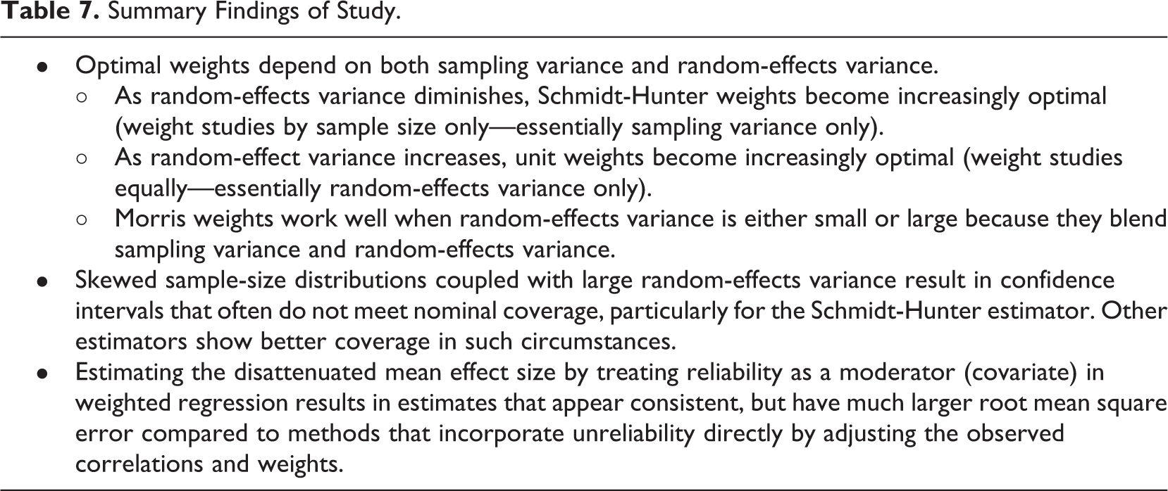
Table 6 also shows the application of each estimator to the overall mean effect size for each of the three studies. Although we should not expect large differences in most cases, given the magnitude of the typical effect size and the typical credibility interval, differences in means and confidence intervals are sufficiently large so as to be consequential depending on the intended inference. Note that for the Rabl, Jayasinghe, Gerhart, and Kühlmann (2014) data, the confidence interval estimates for the Schmidt-Hunter method show virtually no overlap with the intervals from the other methods. Table 7 shows a summary of the main conclusions of the study.

Table 7.

Summary Findings of Study.

Optimal weights depend on both sampling variance and random-effects variance.

As random-effects variance diminishes, Schmidt-Hunter weights become increasingly optimal (weight studies by sample size only—essentially sampling variance only).

As random-effect variance increases, unit weights become increasingly optimal (weight studies equally—essentially random-effects variance only).

Morris weights work well when random-effects variance is either small or large because they blend sampling variance and random-effects variance.

Skewed sample-size distributions coupled with large random-effects variance result in confidence intervals that often do not meet nominal coverage, particularly for the Schmidt-Hunter estimator. Other estimators show better coverage in such circumstances.

Estimating the disattenuated mean effect size by treating reliability as a moderator (covariate) in weighted regression results in estimates that appear consistent, but have much larger root mean square error compared to methods that incorporate unreliability directly by adjusting the observed correlations and weights.

Study Limits

As with any simulation study, the current study was based on assumptions about the data and underlying distribution of effect sizes. Data were randomly drawn from known populations with approximately normal and with skewed distributions for the underlying parameters, but only sampled multivariate normal for the observed data used to compute observed correlations. The simulation used fixed values of the underlying parameters ( $\bar{ρ}$ ,σ_ρ) and fixed values of the number of studies (k). We sampled from previously used distributions of reliabilities for the predictor and criterion, and the data conformed to the assumptions of classical reliability theory. The sample sizes were randomly drawn from a skewed distribution that was intended to represent actual data. It is possible that different choices of parameters would give different results (Hafdahl & Williams, 2009).

We did not simulate range restriction, so researchers wishing to apply the Morris estimator to psychometric meta-analysis with range restriction corrections may want to seek additional justification. Because we did not incorporate artifacts beyond reliability, we do not have information about their influence on bias, efficiency, or coverage.

Conclusion

The Morris estimator appears to offer the benefits of the Schmidt-Hunter approach without its drawbacks for the meta-analysis of the correlation coefficient. Overall, the Morris estimator demonstrates several desirable statistical properties (reasonable values of bias, efficiency and coverage; comparable credibility values) and in many cases, demonstrates superior properties compared to other widely used estimators (Hedges, Schmidt-Hunter). Because of its properties and ease of use with conventional software, the Morris estimator presents itself as an attractive alternative method for meta-analysts working with correlation coefficients.

Supplemental Material

Supplemental Material, Online_Appendix_ORM_741966 - Bias and Precision of Alternate Estimators in Meta-Analysis: Benefits of Blending Schmidt-Hunter and Hedges Approaches

Supplemental Material, Online_Appendix_ORM_741966 for Bias and Precision of Alternate Estimators in Meta-Analysis: Benefits of Blending Schmidt-Hunter and Hedges Approaches by Michael T. Brannick, Sean M. Potter, Bryan Benitez, and Scott B. Morris in Organizational Research Methods

Footnotes

Acknowledgments

The authors thank Deniz S. Ones, Brenton M. Wiernik, Jack W. Kostal, and two anonymous reviewers for comments on drafts of the manuscript.

Declaration of Conflicting Interests

The author(s) declared no potential conflicts of interest with respect to the research, authorship, and/or publication of this article.

Funding

The author(s) received no financial support for the research, authorship and/or publication of this article.

Supplemental Material

Supplemental material for this article is available online.

References

Azzalini

(2016). The R package “sn”: The Skew-Normal and Skew-t distributions (version 1.4-0). Retrieved from http://azzalini.stat.unipd.it/SN

Bonett

D. G.

(2008). Meta-analytic interval estimation for Pearson correlations. Psychological Methods, 13, 173–189.

Bonett

D. G.

(2010). Varying coefficient meta-analytic methods for alpha reliability. Psychological Methods, 15, 368–385.

Borenstein

Hedges

L. V.

Higgins

J. P.

Rothstein

H. R.

(2009). Introduction to meta-analysis. West Sussex, UK: Wiley.

Brannick

M. T.

(2006, 8). Comparison of sample size and inverse variance weights for the effect size. Paper presented at the meeting of the Society for Research Synthesis Methodology, Cambridge, UK.

Brannick

M. T.

Hall

S. M.

(2001, 4). Reducing bias in the Schmidt-Hunter meta-analysis. Paper presented at the meeting of the Society for Industrial and Organizational Psychology, San Diego, CA.

Brannick

M. T.

Yang

Cafri

(2011). Comparison of weights for meta-analysis of r and d under realistic conditions. Organizational Research Methods, 14, 587–607.

Corey

D. M.

Dunlap

W. P.

Burke

M. J.

(1998). Averaging correlations: Expected values and bias in combined Pearson rs and Fisher’s z transformations. Journal of General Psychology, 125(3), 245–261.

DeGeest

D. S.

Schmidt

F. L.

(2010). The impact of research synthesis methods on industrial–organizational psychology: The road from pessimism to optimism about cumulative knowledge. Research Synthesis Methods, 1(3), 185–197.

10.

Field

A. P.

(2001). Meta-analysis of correlation coefficients: A Monte Carlo comparison of fixed- and random-effects methods. Psychological Methods, 6(2), 161–180.

11.

Field

A. P.

(2005). Is the meta-analysis of correlation coefficients accurate when population correlations vary? Psychological Methods, 10(4), 444–467. doi:10.1037/1082-989X.10.4.444

12.

Field

A. P.

Gillett

(2010). How to do a meta-analysis. British Journal of Mathematical and Statistical Psychology, 63, 665–694.

13.

Fife

D. A.

Hunter

M. D.

Mendoza

J. L.

(2016). Estimating unattenuated correlations with limited information about selection variables: Alternatives to Case IV. Organizational Research Methods, 19(4), 593–615.

14.

Fife

D. A.

Mendoza

J. L.

Terry

(2013). Revisiting Case IV: A reassessment of bias and standard errors of Case IV under range restriction. British Journal of Mathematical and Statistical Psychology, 66, 521–542.

15.

Hafdahl

A. R.

Williams

M. A.

(2009). Meta-analysis of correlations revisited: Attempted replication and extension of Field’s (2001) simulation studies. Psychological Methods, 14(1), 24–42.

16.

Hall

S. M.

Brannick

M. T.

(2002). Comparison of two random-effects methods of meta-analysis. Journal of Applied Psychology, 87(2), 377–389.

17.

Hedges

L. V.

Olkin

(1985). Statistical methods for meta-analysis. Orlando, FL: Academic Press.

18.

Hedges

L. V.

Vevea

J. L.

(1998). Fixed- and random-effects models in meta-analysis. Psychological Methods, 3, 486–504.

19.

Higgins

J. P.

Thompson

S. G.

Spiegelhalter

D. J.

(2009). A re-evaluation of random-effects meta-analysis. Journal of the Royal Statistical Society: Series A (Statistics in Society), 172, 137–159.

20.

James

L. R.

Demaree

R. G.

Mulaik

S. A.

(1986). A note on validity generalization procedures. Journal of Applied Psychology, 71, 440–450.

21.

Law

K. S.

(1995). The use of Fisher’s z in Schmidt-Hunter-type meta-analyses. Journal of Educational and Behavioral Statistics, 20(3), 287–306.

22.

Law

K. S.

Schmidt

F. L.

Hunter

J. E.

(1994). A test of two refinements in procedures for meta-analysis. Journal of Applied Psychology, 79(6), 978–986.

23.

I.-S.

Schmidt

F. L.

Wooldridge

C. D.

(2016). Correction for range restriction in meta-analysis revisited: Improvements and implications for organizational research. Personnel Psychology, 69, 975–1008. doi:10.1111/peps.12122

24.

Schmidt

F. L.

(2006). Correcting for indirect range restriction in meta-analysis: Testing a new meta-analytic procedure. Psychological Methods, 11(4), 416–438.

25.

Lipsey

M. W.

Wilson

D. B.

(2001). Practical meta-analysis. Thousand Oaks, CA: Sage.

26.

Mason

Allam

Brannick

M. T.

(2007). How to meta-analyze coefficient of stability estimates: Some recommendations based on Monte Carlo studies. Educational and Psychological Measurement, 67, 765–783.

27.

McEvoy

G. M.

Cascio

W. F.

(1987). Do good or poor performers leave? A meta-analysis of the relationship between performance and turnover. Academy of Management Journal, 30(4), 744–762.

28.

Morris

S. B.

Daisley

R. L.

Wheeler

Boyer

(2015). A meta-analysis of the relationship between individual assessments and job performance. Journal of Applied Psychology, 100(1), 5–20.

29.

Paterson

T. A.

Harms

P. D.

Steel

Credé

(2016). An assessment of the magnitude of effect sizes: Evidence from 30 years of meta-analysis in management. Journal of Leadership & Organizational Studies, 23(1), 66–81. doi:10.1177/1548051815614321

30.

Pearlman

Schmidt

F. L.

Hunter

J. E.

(1980). Validity generalization results for tests used to predict job proficiency and training success in clerical occupations. Journal of Applied Psychology, 65, 373–406.

31.

Rabl

Jayasinghe

Gerhart

Kühlmann

T. M.

(2014). A meta-analysis of country differences in the high-performance work system–business performance relationship: The roles of national culture and managerial discretion. Journal of Applied Psychology, 99(6), 1011–1041.

32.

Raudenbush

S. W.

(2009). Analyzing effect sizes: Random-effects models. In Cooper

H. C.

Hedges

L. V.

Valentine

J. C.

(Eds.), The handbook of research synthesis and meta-analysis (2nd ed., pp. 295–315). New York, NY: Russell Sage Foundation.

33.

Rothstein

H. R.

Sutton

A. J.

Borenstein

(2005). Publication bias in meta-analysis: Prevention, assessment and adjustments. Chichester, UK: Wiley.

34.

Sanchez-Meca

Marin-Martinez

(2008). Confidence intervals for the overall effect size in random-effects meta-analysis. Psychological Methods, 13(1), 31–48.

35.

Schmidt

F. L.

Hunter

J. E.

(2015). Methods of meta-analysis (3rd ed.). Thousand Oaks, CA: Sage.

36.

Schulze

(2004). Meta-analysis: A comparison of approaches. Cambridge, MA: Hogrefe and Huber.

37.

Schulze

(2007). Current methods for meta-analysis: Approaches, issues and developments. Journal of Psychology, 215, 90–103.

38.

Shadish

W. R.

Haddock

C. K.

(2009). Combining estimate of effect size. In Cooper

Hedges

L. V.

Vanentine

J. C.

(Eds.), The handbook of research synthesis and meta-analysis (2nd ed., pp. 257–277). New York, NY: Russell Sage Foundation.

39.

Silver

N. C.

Dunlap

W. P.

(1987). Averaging correlation coefficients: Should Fisher’s z transformation be used? Journal of Applied Psychology, 72(1), 146–148.

40.

Steel

(2013, 6). Converting between meta-analytic variance estimates based on correlations and Fisher z. Paper presented at the annual meeting of the Society for Research Synthesis Methodology Providence, RI.

41.

Steel

Kammeyer-Mueller

J. D.

(2002). Comparing meta-analytic moderator estimation techniques under realistic conditions. Journal of Applied Psychology, 87(1), 96–111. doi:10.1037/0021-9010.87.1.96

42.

Steel

Kammeyer-Mueller

J. D.

Paterson

T. A.

(2015). Improving the meta-analytic assessment of effect size variance with an informed Bayesian prior. Journal of Management, 41(2), 718–743. doi:10.1177/0149206314551964

43.

Thomas

(1990). A likelihood-based model for validity generalization. Journal of Applied Psychology, 75, 13–20.

44.

Thompson

S. G.

Higgins

J. P. T.

(2002). How should meta-regression analyses be undertaken and interpreted? Statistics in Medicine, 21, 1559–1573. doi:10.1002/sim.1187

45.

Veroniki

A. A.

Jackson

Viechtbauer

Bender

Bowden

Knapp

G.,

Salanti

(2015). Methods to estimate the between-study variance and its uncertainty in meta-analysis. Research Synthesis Methods, 7, 55–79.

46.

Viechtbauer

(2005). Bias and efficiency of meta-analytic variance estimators in the random-effects model. Journal of Educational and Behavioral Statistics, 30(3), 261–293.

47.

Viechtbauer

(2010). Conducting meta-analyses in R with the metafor package. Journal of Statistical Software, 36(3), 1–48.

Supplementary Material

Please find the following supplemental material available below.

For Open Access articles published under a Creative Commons License, all supplemental material carries the same license as the article it is associated with.

For non-Open Access articles published, all supplemental material carries a non-exclusive license, and permission requests for re-use of supplemental material or any part of supplemental material shall be sent directly to the copyright owner as specified in the copyright notice associated with the article.

0.00 MB

0.03 MB

0.20 MB