
Abstract
Theories suggest that groups within organizations often develop shared values, beliefs, affect, behaviors, or agreed-on routines; however, researchers rarely study predictors of consensus emergence over time. Recently, a multilevel-methods approach for detecting and studying emergence in organizational field data has been described. This approach—the consensus emergence model—builds on an extended three-level multilevel model. Researchers planning future studies based on the consensus emergence model need to consider (a) sample size characteristics required to detect emergence effects with satisfactory statistical power and (b) how the distribution of the overall sample size across the levels of the multilevel model influences power. We systematically address both issues by conducting a power simulation for detecting main and moderating effects involving consensus emergence under a variety of typical research scenarios and provide an R-based tool that readers can use to estimate power. Our discussion focuses on the future use and development of multilevel methods for studying emergence in organizational research.
In their classic work, The Social Psychology of Organizations, Daniel Katz and Robert Kahn (1978) suggested that the essence of an organization is “patterned” human behavior. Building on this idea, organizational research frequently describes and defines groups through attributes such as shared values, affect, common behaviors, or procedures on which the organizational or group members have developed. One important question for organizational research is how the psychological essence of organizations and groups—such as shared values and common behavior patterns—develop through interactions among unit members.
Researchers have used different terms to formally describe patterns of change associated with social interactions. One frequently used term is emergence (Cronin & Weingart, 2011; Dansereau, Yammarino, & Kohles, 1999; Felin, Foss, & Ployhart, 2015; Humphrey & Aime, 2014; Kozlowski, 2015; Kozlowski, Chao, Grand, Braun, & Kuljanin, 2013; Morgeson & Hofmann, 1999; Ployhart & Moliterno, 2011). Emergence generally indicates an increase in similarity, agreement, or commonality among unit members that leads to the formation of a shared climate (Ashforth, 1985); however, the term emergence can be interpreted more broadly to imply the creation of any new property. Within this broad conceptualization of emergence, an extended range of phenomena is possible, including the formation of a state of dissensus—an important process less frequently studied in the organizational literature (Harrison & Klein, 2007; Mathieu, Tannenbaum, Donsbach, & Alliger, 2014). Given these potential definitional ambiguities, we use the narrow term consensus emergence to describe increases in shared values, opinions, or behaviors over time and the term dissensus to refer to a pattern of decreased similarity in outcome variables. We use the term emergence more generally to refer to patterns of change associated with either consensus or dissensus emergence.
One challenge for organizational researchers studying emergence is that the process both unfolds over time and is simultaneously a multilevel group phenomenon. This inherent complexity requires a methodological approach that accounts for change over time within higher-level entities and that captures gradual increases (or decreases) in consensus over time. In contrast, organizational multilevel research has generally been confined to assessing the amount of emergence among unit members at snapshots in time using cross-sectional multilevel statistics such as the intraclass correlation, type 1 (ICC1; Bliese, 2000). For instance, at first glance, a sample of groups with an ICC1 of .02 at Time 1 (T1), an ICC1 of .15 at Time 2 (T2), and an ICC1 of .20 at Time 3 (T3) would appear to be showing a pattern of consensus emergence. Later we describe why it is problematic to interpret raw ICC1 values across time as done here.
Recently, researchers have described an extended three-level multilevel modeling approach—the consensus emergence model (CEM)—that allows researchers to systematically model emergence in the multilevel framework and study organizational and group characteristics that predict emergence (Lang & Bliese, 2018; Lang, Bliese, & Adler, 2019; Lang, Bliese, & de Voogt, 2018). For instance, an initial study applied the CEM approach to archival data from U.S. Army companies undergoing a major change in core technology and showed that a shared climate of job satisfaction emerged among company members over time (Lang et al., 2018). That is, the finding was focused not on how job satisfaction increased or decreased; rather, the focus was on how soldiers within companies become more similar to each other over time.
The CEM approach can potentially be used to investigate a wide variety of organizational research questions. Nonetheless, three open questions remain for organizational researchers who plan future studies on emergence. First are questions about sample sizes needed to detect emergence effects with satisfactory statistical power. An initial article on consensus emergence briefly explored this issue by running a power simulation under a typical scenario using 10, 20, and 30 groups. These initial findings suggested that 20 groups were needed (Lang et al., 2018); however, sample size questions are more complex than captured by Lang et al. (2018) because statistical power may be impacted by combinations of different distributional properties—specifically how observations are distributed across different group sizes, the number of groups, and the overall number of observations. A second related question centers on determining what effect sizes can be detected under different distributional properties, and the third question pertains to how predictors of emergence (e.g., moderation effects) respond to different distributional properties. In this article, we systematically address these questions by conducting a comprehensive power simulation of emergence effects under a variety of common scenarios. We supplement our simulations with the description of a tool written in the R statistical language that readers can use to conduct power simulations for emergence effects.
An Illustrative Example
Table 1 includes a prototypical data set with 10 units with five members across three timepoints. The measurements were conducted on a Likert scale ranging from 1 (strongly disagree) to 5 (strongly agree) with multiple items. The 10 units differ on the basis of a group-level predictor.
Example Dataset.

A hypothetical example where researchers might encounter a data set of this type would be perceptions of procedural justice in newly formed work groups that work under pay systems that differ in flexibility. For the purposes of illustration, assume we have access to a continuous pay system rating scale where low values represent low flexibility and high values represent high flexibility. Several researchers have argued that justice perceptions in groups may lead to emergence effects because perceptions of organizational injustice may be contagious (Degoey, 2004; Ehrhart, 2004; A. Li & Cropanzano, 2009; Liao & Rupp, 2005). The underlying idea is that people have a tendency to compare and validate their own emotional reactions to stressful events with others (Barsade, 2002). This validation process may lead to consensus about how events (i.e., events related to fairness) should be interpreted. Researchers have long been interested in contagion effects in organizational field data, but statistically showing these types of effects in field data has been challenging, so existing data often come from the laboratory (Ambrose, Harland, & Kulik, 1991; A. Li & Cropanzano, 2009). We use the term contagion in this context because there is no explicit goal to form consensus; hence, consensus formation is not deliberate. Researchers may also be interested in consensus in groups where the explicit goal is to come to consensus. As examples, juries deliberate to form a joint opinion (Lang et al., 2019), and teams may need to agree about a negotiation strategy.
Figure 1 shows a prototypical emergence pattern with individual measurements increasingly moving closer to the group trend over time. The figure illustrates a form of heteroscedasticity where the variance among group members is dramatically decreasing. In the CEM, this pattern of variance change is treated as a substantive variable that can be formally tested and predicted. The strong effects in Figure 1 (while illustrative) are not realistic in most organizational data. Figure 2 provides a more realistic pattern for 10 teams—several of the groups (Units 4, 5, 6, and 9) appear to show evidence of a consensus emergence pattern. Over time, the responses seem to move closer to the average opinion of the group, but it is not clear how large the effect is or whether the observed pattern would be statistically significant for the sample as a whole. In the next section, we show how the CEM can be used to formally test the hypothesis that a consensus emergence pattern exists in the data in Table 1 and Figure 2.

Example for a prototypical consensus emergence pattern.
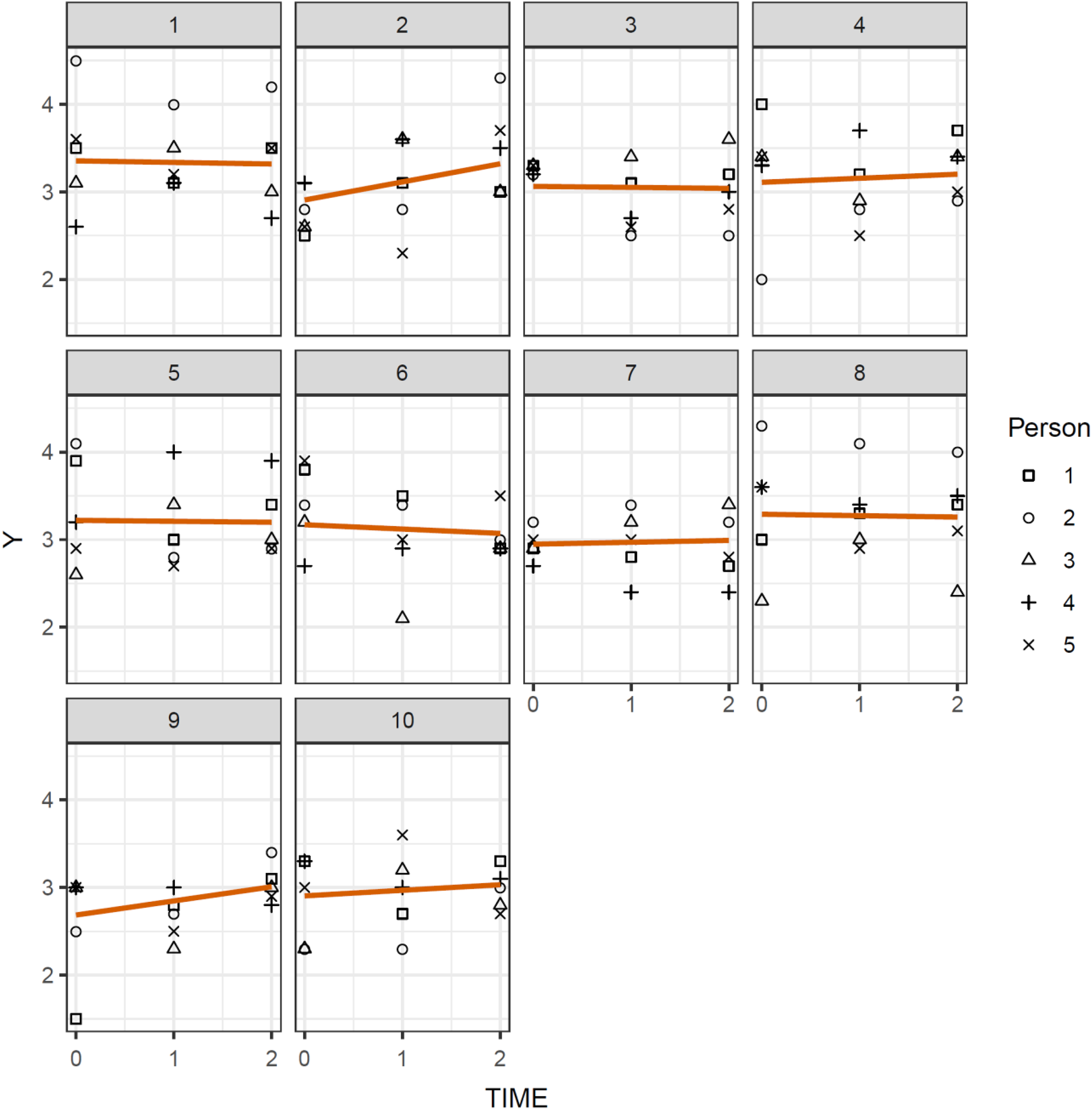
Plot of the example dataset in Table 1.
The Consensus Emergence Model
We previously noted that a frequently used tool for assessing the presence of consensus in cross-sectional data is the ICC1. Unfortunately, the ICC1 has two severe limitations for modeling consensus emergence over time that make it poorly suited for detecting consensus emergence patterns in data such as the illustrative data set shown in Table 1.
One limitation of the ICC1 is evident in the formula for the ICC1. This formula is based on a basic intercept-only multilevel model (Yij = γ00 + u0j + eij where Y is the response, i the unit member, j the unit, γ00 the intercept, u0j the latent group mean, and eij the residual). The formula (ICC1 = τ00 / [τ00 + σ2]) defines the ICC1 as the variance, τ00, of the latent group means (u0j) divided by itself plus the variance, σ2, of the residuals (eij); in other words, the percentage of variance that group membership explains in the overall variance. The problem is that the ICC1 cannot effectively be used to track changes in emergence over time because two different process can lead to increases in ICC1: either (a) change in the variance of the latent group means (an increase or reduction in τ00) or (b) change in the amount of similarity that group members show with the group mean (an increase or decrease in σ2).
Empirical ICC1 values tracked over time frequently fail to show emergence patterns (Allen & O’Neill, 2015)—possibly because changes in τ00 along with simultaneous changes in σ2 work against detecting these types of patterns. A pattern of simultaneous change in τ00 and σ2 applies to the example data in Table 1 and Figure 2. The ICC1 values for these data at T1, T2, and T3 were .11, .02, and .02, respectively. These values do not imply a consensus emergence effect even though Figure 2 seems to provide evidence for an effect of this type.
The second limitation of the ICC1 is that it does not provide a comprehensive modeling framework for studying emergence. To conduct effective research on emergence phenomena, researchers would benefit from a formal statistical test for the presence of emergence, effect size information, and the ability to test for moderators of emergence effects.
The limitations of the ICC1 were the main motivation for the development of the CEM (Lang & Bliese, 2018; Lang et al., 2018). The CEM addresses the limitations of the ICC1 and the need for a modeling framework to formally test for consensus emergence using an extended three-level multilevel model specification. The basic CEM can be written as follows.


In these equations, t refers to the measurement occasion, i refers to the unit-member (typically individuals), and j refers to the unit. The model combines the basic model structure of the intercept-only model for the ICC1 with a growth model that accounts for changes (u10j) in the latent unit-means (u00j) along with change in the between group variance over time (captured by υ01, and υ11). The model accounts for the fact that each unit-member provides multiple ratings through the unit-member-specific variance (τ00). The resulting three-level model includes measurements at level-1 nested in unit-members at level-2, and unit-members at level-2 nested in units (i.e., groups) at level-3.
The model is extended in the sense that it goes beyond the standard multilevel models and uses a variance function (σ2exp[2δ1TIMEt]) to model change in the residual variance over time (Culpepper, 2010; Harvey, 1976; Pinheiro & Bates, 2000; Rutemiller & Bowers, 1968). In organizational research and other social sciences, variance functions have usually been included in multilevel models and other regression models to account for potential violations of the homogeneity of residual variance assumption (Bliese & Ployhart, 2002; Culpepper, 2010; Harvey, 1976; Rutemiller & Bowers, 1968; Singer & Willett, 2003). However, research methods experts have long realized that changes in residual variance functions can also have substantive meaning and can thus be used to gain substantive insights (Goldstein, 2011; Kim & Seltzer, 2011; Pinheiro & Bates, 2000; Raudenbush, 1988). Building on this earlier work, the CEM uses an exponential variance function to account for the gradual increases or decreases in residual variance among unit-members. One advantage of using an exponential variance function is that it yields an effect size estimate, δ1, that corresponds to an approximate linear increase or decrease in the residual standard deviation σ (square root of the residual variance). 2 That is, when the time variable TIME is coded so that it increases by 1 with each measurement occasion t (e.g., 0, 1, 2,…), δ1 approximately captures the percent change in the residual standard deviation with each measurement occasion up to about +/- .20 (or 20% change) after which the interpretation is not quite as direct.
In research on consensus emergence, δ1 is expected to be negative implying a reduction in the residual standard deviation. For instance, when σ is 2.6, δ1 is -0.06, and TIME runs from 0 to 2, the formula for the residual variance at the three measurement occasions would be σ2 = 2.62×exp(2×-0.06×0) = 6.76, σ2 = 2.62×exp(2×-0.06×1) = 6, and σ2 = 2.62×exp(2×-0.06×2) = 5.32, respectively. Taking the square root of the variance, the change pattern in the residual standard deviation is σ = 2.60, σ = 2.45, and σ = 2.31 which is approximately equivalent to a six percent decrease with each measurement occasion (2.45 is 94% of 2.60). To test the significance of δ1, researchers can use a loglikelihood ratio test that compares a model without the exponential variance function (or δ1 = 0) with the basic CEM specification shown in Equation 1-6.
The CEM model can be fit in several advanced multilevel modeling software packages like the nlme package (Pinheiro & Bates, 2000) in the R environment (R Core Team, 2018) and Mplus (Lang et al., 2018). Typically, restricted maximum likelihood (REML) estimation is preferred because the δ1 effect is a component of the variance portion of the model, and REML is considered more accurate for estimating variance components where fixed-effects remain constant as they do in the CEM model (Pinheiro & Bates, 2000; Singer & Willett, 2003).
While the ICC1 has limitations as a measure of consensus emergence, it has the desirable property of providing information that can be readily interpreted by researchers as the percentage of variance that group membership explains in the overall variance at specific points in time. In some cases, researchers may therefore be interested in translating information from a CEM-based analysis into ICC values for particular points in time to evaluate the degree of overall emergence. This goal can be achieved using the ICCEM coefficient (Lang & Bliese, 2018):

In interpreting ICCEM values, researchers can follow existing guidance on interpreting ICC1 values (Bliese, 2000; Bliese, Maltarich, Hendricks, Hofmann, & Adler, 2019; LeBreton & Senter, 2008). A desirable feature of the ICCEM is that it is model-based and thus more robust and stable than ICC1 values at particular points in time.
While δ1 values provide an approximate relative measure of change and ICCEM values provide a measure of emergence at particular points in time, researchers may also be interested in an overall measure of effect size or explained variance for emergence effects. A challenge for models that include change in the residual variance is that most approaches for estimating R2 values in mixed-effects models build on the residuals so that these R2 values either do not change or they decrease when changes in residual variances are included (see overviews in LaHuis, Hartman, Hakoyama, & Clark, 2014; Rights & Sterba, 2019). Thus, typical R2 approaches are not useful for extended multilevel mixed-effects models. A solution is to use a generalized R2 statistic such as the

The basic CEM shown in Equation 1-6 above can be relatively easily extended to allow researchers to test for potential effects of moderators on consensus emergence. More specifically, substituting Equation 3 and 4 against the following Equations 9 and 10, respectively, yields a model that tests the effect of a unit-level predictor on emergence.


In using this type of model, researchers should be aware that the CEM is a type of growth model and thus the unit-level predictor should be stable (Ployhart & Kim, 2013; Singer & Willett, 2003). The model is flexible in the sense that the predictor in the model can either be dichotomous or continuous. The interpretation of the δ2 and δ3 parameters in the model are analogous to the interpretation of interaction effects in normal regression analyses: δ2 captures the main effect of the predictor at baseline (when TIME is coded 0 at T1), and δ3 captures differences in the consensus emergence effect δ1 for different levels of the predictor.
CEM Analysis of the Illustrative Example
To illustrate the use of the CEM, Table 2 provides the results of a CEM analysis of the illustrative data in Table 1. As shown in Table 2, a consensus emergence effect is present in this dataset, δ1 = -0.22. The log-likelihood comparison test between a model without consensus emergence and the CEM suggests that this effect is significant, χ2 (df = 1, N = 150) = 5.10, p = .02. The significant TIME × PRED interaction effect, δ3 = 0.44, χ2(df = 1, N = 150) = 11.22, p < .01, in the residual part of Model 4 in Table 2 also indicates that the environment variable (”PRED” – pay system flexibility in our earlier example) moderates the consensus emergence effect so that the effect over time is stronger when pay system flexibility is high. While hypothetical, these findings suggest that justice contagion is a function of the groups’ pay system flexibility: contagion occurs more strongly in the groups with a flexible payment system than in groups with an inflexible system.
Baseline Model (Model 1), Consensus Emergence Model (Model 2), and Test of a Moderator of Consensus Emergence (Model 3 and Model 4) Fitted to the Example Dataset.

Note. 10 units with 5 unit-members measured at 3 measurement occasions (150 observations).
* p < .05
Researchers interested in further examining the data can estimate the ICCEM for each time point. The ICCEM estimates from the data are .13, .05, and .04 at TIME = 0, TIME = 1, and TIME =2, respectively, and are similar to the ICC1 values of .11, .02, and .02. The CEM analyses in Table 2 illustrate why the ICCEM (and ICC1) values become smaller. Specifically, in this example the negative covariance term (υ01) leads to a decrease in the between-group variance that is more pronounced than the decrease in the within-group variance lowering ICCEM values. We note that in applied examples with many measurement occasions, the ICCEM will often return values that are easier to interpret. Table 2 also includes the
The Power Simulations
Statistical power refers to the long-term probability of detecting a significant effect when the effect is present (Cohen, 1992). A basic convention for statistical power is that it should at least be .80 so a researcher has an 80% chance of detecting the effect. A power analysis commonly includes several steps. In the first step, a researcher chooses an alpha level (e.g., <.05) and a reasonable a-priori expected effect size that seems plausible for the research question on the basis of earlier research and practical considerations (what effect size would be of practical interest). Theoretical considerations may also be of interest but actual information on the magnitude of effect sizes from theory is often rare. After choosing the effect size, the next step is to estimate power for the given effect size. For relatively simple statistical models, it is possible to directly estimate power using formulas (Cohen, Cohen, West, & Aiken, 2003). However, for more complex types of models like multilevel models, power depends on a variety of parameters in the model and their combination so power may more efficiently be estimated using simulations (Bliese & Hanges, 2004; Bolker et al., 2013; Mathieu, Aguinis, Culpepper, & Chen, 2012; Pinheiro & Bates, 2000). In power simulations, the researcher specifies the parameters of the data that he/she expects and then generates a series of datasets from the resulting model using a pseudo random number generator. Because the resulting datasets have been generated from a model for which the underlying parameters are known, power represents the percentage of datasets that return a significant effect when the effect exists.
We conducted two different power simulations. In the first, we focused on detecting consensus emergence effects. For the CEM, the focus was on the log-likelihood-ratio test (χ2 -test) which compared a model with a consensus emergence effect to a model without this effect. The second power simulation focused on detecting moderators of consensus emergence. The focus thus was on the log-likelihood-ratio test contrasting a model with a moderator of the consensus emergence effect to a model without this effect. Multilevel literature commonly states that studies require at least 30 to 50 groups (Hox, 2002; Maas & Hox, 2005; Mathieu et al., 2012; Snijders & Bosker, 1993, 1999); however, these recommendations are generally based on cross-sectional studies and focus on top-down effects and thus apply to situations that fundamentally differ from the CEM. To gain insights into the requirements for the CEM, we manipulated the total sample size, the sample size at the unit level, and how the observations were distributed among units, unit members, and measurement occasions. Simulation conditions were selected to provide insights into designing field studies – for instance whether including additional measurements might compensate for a smaller number of units.
Method
Table 3 shows the data generating values used for the two simulations. The values in both simulations were based on experience with existing data, effect sizes from initial consensus emergence analyses, and theoretical assumptions. Experience suggests that meaningful consensus emergence effects are typically around -.15. For instance, a reanalysis of a study of group cohesion ratings by psychology students working in teams over six weeks (32 groups / 243 persons / 705 observations) yielded an effect size of δ1= -0.15 over three time points (Lang & Bliese, 2018). A reanalysis of a dataset on job satisfaction in 34 Army companies measured three times (471 soldiers and a total of 1,351 observations) originally reported by Bliese and Ployhart (2002) revealed an effect size of δ1= -0.10 (Lang et al., 2018). A more extreme effect size estimate (δ1= -1.02) was obtained in a reanalysis of Sherif’s (1935) classic laboratory study on group norms that included four measurements (see Lang & Bliese, 2018). This group norm study isolated the phenomenon of group norm formation by not providing much additional information to participants: such extreme effect sizes are unlikely in field data. 1
Values Used in the Simulations.
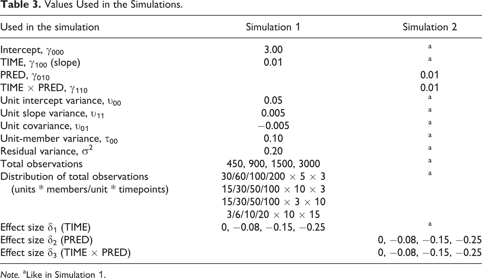
Note. aLike in Simulation 1.
From a theoretical perspective, it seems reasonable to expect that a typical organizational study could yield a reduction of 15 percent of the variance with each measurement occasion across three measurements (45 percent reduction in the residual variance overall). We therefore used δ1 = -0.15 as the moderate effect size, δ1 = -0.08 as a small effect size, and δ1 = -0.25 as a large effect size across three time points for the simulation. Because we were interested in comparing the effects of the number of time points on power, we rescaled the time variable when more time points were included in the study by dividing the time variable for the larger number of measurement occasions by 3 so that the effect sizes were equivalent. For instance, with 10 measurement time points 0, 1, 2, 3, 4, 5, 6, 7, 8, and 9 were rescaled to 0, 1/3, 2/3, 1, 4/3, 5/3, 2, 7/3, 8/3, and 3, respectively so that 10 measurement occasions would also have a 45% overall reduction in the moderate effect size condition. All power simulations were conducted in the R (R Core Team, 2018) environment using the nlme package (Pinheiro & Bates, 2000).
Results
The results of the power simulations are provided in Table 4, and Figures 3 and 4. Notice in both figures that power was mostly dependent on the overall number of data points and the effect size. The large effect size of δ1/δ3 = -0.25 yielded sufficient power across all conditions in both sets of simulations. In the first set of simulations focused on detecting consensus emergence, the moderate effect size of δ1 = -0.15 had acceptable power (> .80) with at least 900 observations no matter how these observations were distributed across units, unit sizes, and time points (see Figure 3). While a value of 900 seems large, consider that 30 groups with ten group members over three measurement occasions produces 900 observations. The small effect size, in contrast, required 3,000 observations to consistently yield sufficient power.
Results of the Simulations.
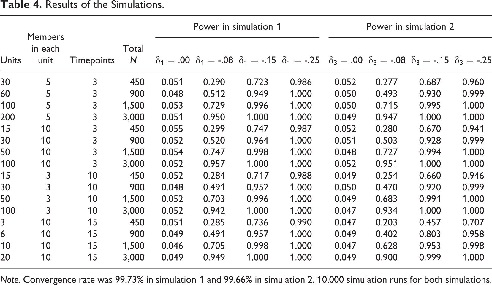
Note. Convergence rate was 99.73% in simulation 1 and 99.66% in simulation 2. 10,000 simulation runs for both simulations.
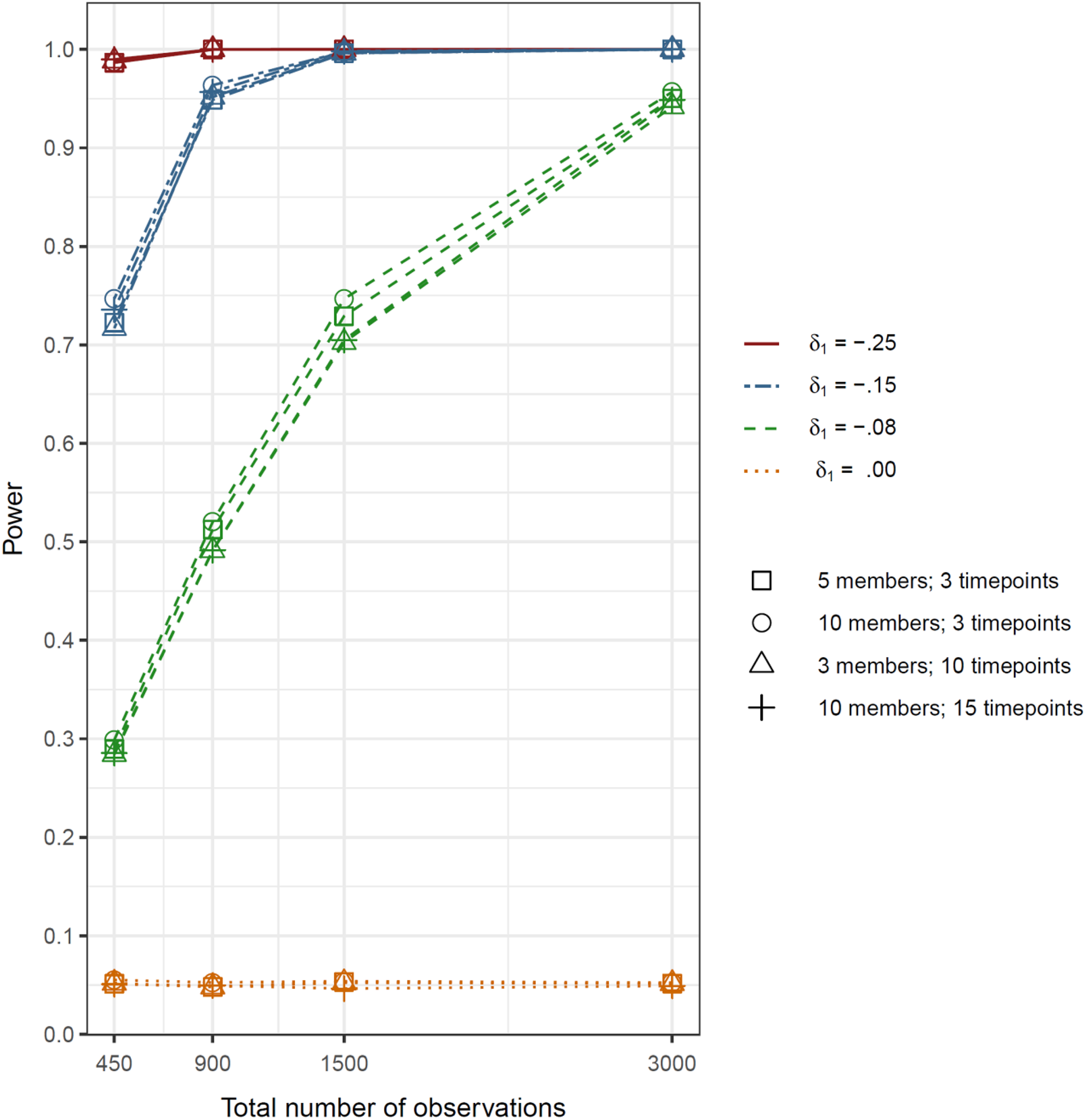
Power to detect a consensus emergence effect as a function of effect size, the total number of observations, and the distribution of the observations over groups and timepoints.

Power to detect a moderator of a consensus emergence effect as a function of effect size, the total number of observations, and the distribution of the observations over groups and timepoints.
In the second set of simulations investigating the power to detect moderators of consensus emergence, the moderate effect size also yielded sufficient power with 900 observations in three of the four conditions (see Figure 4). However, in the fourth condition with a large number of unit-members, and a large number of time points, power was insufficient. The reason is that just 6 groups are not adequate to effectively account for sample size variation of the moderator. In contrast, 10 units were sufficient to generate acceptable power with a large number of measurement occasions (15) and a large number of unit members (10). Again, the small effect size required 3000 observations to consistently yield sufficient power.
Power Simulation Tool
The power simulations cover a set of typical scenarios in organizational research. However, researchers may want to do their own power simulation on the basis of more specific expectations. Appendix B and C provide R code allowing researchers to conduct simulations of this type. The R functions include model components that a researcher can specify a-priori and additionally the setting “tscale” allows researchers to more easily study the impact of varying numbers of time points without changing the metric of the values entered into the model. tscale simply rescales the time variable to make scenarios comparable. For instance, if a researcher wants to compare a scenario with 9 or 3 time points, he/she enters tscale=3 in the model with 9 time points so that all other data generating values for the simulation are equivalent.
Discussion
Emergence represents a multilevel process describing how lower-level units change over time to form characteristics of higher-level units. The concept of emergence plays several roles in theory development and in advancing research. First, emergence often provides the theoretical foundation for aggregating responses to higher-levels and conducting research using higher-level constructs. That is, demonstrating that emergent processes occur for specific constructs represents an important aspect of the multilevel construct validation process that help justifies aggregation (Bliese et al., 2019).
Second, on a related note, examining emergence via the CEM can provide a deeper understanding of existing unit-level constructs. For instance, unit-level constructs like justice climate or safety climate (e.g., Zohar, 2010) are well-established predictors of organizational outcomes. As a field, however, organizational research does not currently know if justice climates and safety climates develop through emergent processes where unit members become more similar over time with relatively little mean change across units, or whether safety climates develop because units becoming more extreme in term of mean differences. That is, a significant ICC value at one time point does not provide information about the process that produced it.
Third, the ability to model predictors provides a way to develop and test procedures to predict emergence. Again, using the example of safety climate, researchers and practitioners could determine whether a specific training program causes units to more quickly develop shared safety climates. A study of this nature would be interested in mean change over time, but in addition to mean change, it would be important to examine patterns of emergence among unit members with an eye towards enhancing consensus. As another example, research could also be framed around understanding why some group members become more divergent over time and incorporate predictors of these divergent patterns. Work in this area is important because a lack of consensus among group members is presumably an index of a poorly functioning team.
In the end, studies of emergence potentially have much to offer in terms of theory development. Like other areas of research, studies of emergence need to have acceptable statistical power to help advance knowledge. We used simulation studies to examine how the statistical power of the CEM was related to differences in overall sample sizes, the number of groups, group size, and the number of time points. In addition, we provide R-based tools that researchers can use to conduct power simulations. Our results suggest that the power of the CEM mainly depends on the overall number of data points and the effect size. The distribution of data points across units, time, and unit-members generally appears to have a limited influence on the results. An important exception is that power to detect moderation is substantially lowered by having a small number of units in combination with a high number of measurement occasions and unit members. In this scenario, the large number of measurement occasions and unit members cannot compensate for the lack of information related to the moderator due to the small number of units.
Overall, the results suggest that in many situations a relatively small number of groups may be sufficient when there are either many group members or many measurements for detecting consensus emergence. These results are encouraging in suggesting that datasets that include a limited number of groups can potentially be used to generate novel and interesting insights when frequent measurements are possible. The results may also open the door for studies that track a small number of groups for an extended period of time to see whether group members come together to gain insights on group functioning. An initial example for a study of this type is a diary study that tracked a small number of groups of archeologists on a field mission over several weeks (Lang et al., 2018). The results also suggest that the sample size requirements for detecting emergence are lower than for other types of multilevel effects like, for instance, cross-level moderation effects (Maas & Hox, 2005; Mathieu et al., 2012; Snijders & Bosker, 1993, 1999).
Limitations
We note several limitations of this work. One limitation relates to the nature of the model on which we focused in this article—the consensus emergence model (CEM). The CEM fundamentally assumes that changes in the residual variance convey important and relevant information about emergence, and that patterns of variance change are manifest reflections of changes in group climate. We see the CEM as complementing other approaches and note that the literature on emergence has described several other types of emergence phenomena and alternative methods to study these complex phenomena. Other models to study emergence include qualitative research methods (Gehman, Trevino, & Garud, 2013), computational models that simulate complex emergence processes to gain insights into plausible explanations for empirical patterns (Kozlowski et al., 2013), and network models (Fowler & Christakis, 2008). A review of these methods is beyond the scope of this article but interested readers may examine reviews and overviews of these methods (Kozlowski et al., 2013; Lang et al., 2018). We believe that these alternative methods will complement the multilevel approach for studying emergence.
We also note that a limitation of the CEM is that it—like all linear mixed-effect multilevel models—assumes normally distributed residuals. This assumption does not mean that the dependent variable itself needs to be normally distributed; rather, the assumption is that the residuals of the model are approximately normally distributed after accounting for all model components. In practice, the assumption of normally distributed residuals implies that users of the CEM should be cautious because heavily skewed data with strong floor and ceiling effects can violate the assumption of normally distributed residuals. A recommended strategy is to examine the residuals using graphical model checking procedures (Pinheiro & Bates, 2000).
Finally, a specific limitation of our study is the fact that we only examined a limited set of conditions so our power simulations will likely not cover some situations that researchers will face in their research. Nonetheless, we attempted to test scenarios that reflected common data characteristics with respect to factors such as group size, the number of measurement occasions, and the number of groups. In addition, the R code in the Appendices B and C can be used to conduct power simulation studies tailored to the specific attributes of the research setting.
Future Directions
One area for future research could be to extend the CEM to study more complex phenomena. One possible extension is to include more complex types of change. The analyses we considered in this study were limited to linear change in both latent group means and consensus. Change, however, may show forms such as a quadratic emergence trajectory where a group first becomes more homogenous and then more heterogeneous (e.g., Tuckman & Jensen, 1977). Change in consensus could also be discontinuous (Bliese & Lang, 2016; Singer & Willett, 2003) because a catalyst event could occur in a group and lead to a pattern of either consensus or dissensus. These more complex consensus change models can be specified relatively easily using the procedures described in this paper by adding the respective change terms both in the fixed effects part (e.g.,
Another potential extension of the CEM is to include additional complexity in the consensus change part of the model. For instance, it is possible to add an additional level of analysis to the CEM to account for measurement error (Lang et al., 2018). This approach requires one to use a somewhat different parametrization of variance function models (Goldstein, 2005, 2011) that is not as easy to interpret as the parametrization with the exponential variance functions we generally recommend, but can be fit in almost all multilevel software packages. To implement this approach, one adds time as a predictor centered at the end of the observation period [TIMEt – max(TIMEt)] at the person level (now Level 2 because of the additional level of nesting) and specifies that the time variable is uncorrelated with the intercept. The advantage of this alternative model is also that it allows both the intercept and the slope to vary across individuals with the assumption that both are from a normal distribution (random effects). A somewhat similar approach pursued by researchers is to directly add a random intercept effect to the exponential variance specification for the residual variance (Culpepper, 2010; X. Li & Hedeker, 2012). These types of models typically do not include random slopes for time like the CEM but have the advantage that they can even be fit with a joint random effects distribution so that the random error variability can be correlated with the other random effects in the model. Although interesting, these more complex models are frequently not easy to fit for three-level structures and may run into convergence problems unless the sample size is very large (X. Li & Hedeker, 2012; Nestler, Geukes, & Back, 2018). Ultimately, it is important for researchers to carefully balance model complexity and model parsimony (Bates, Kliegl, Vasishth, & Baayen, 2015; Matuschek, Kliegl, Vasishth, Baayen, & Bates, 2017).
From a theoretical perspective, it may be interesting to use the CEM to capture more complex forms of emergence. One way this can already be done within the framework of the CEM is to add dichotomous predictors (e.g., leaders vs. non-leaders or ethnic minority vs. non-ethnic minority, or male vs. female) that separate subgroups within groups from each other. For instance, a recent article provides an illustration of how to test consensus emergence among minority and majority group members in mock juries (Lang et al., 2019). We anticipate opportunities to extend the model by looking at other predictors associated with group members.
A set of final questions for future research center on how the CEM can be combined with other established techniques in the multilevel literature like multi-membership models (Cafri, Hedeker, & Aarons, 2015) or mediation models (MacKinnon, Fairchild, & Fritz, 2007). Multi-membership models allow persons to be members of multiple groups. We are not aware of work examining how multi-membership affect emergence. Mediation models are frequently discussed in the literature but it is not clear how the approach could be extended to emergence models. Even with this limitation, however, we note that the ability to include group-level predictors provides a potentially powerful way to examine mechanisms that lead to emergence. Indeed, researchers have argued that one possible approach for testing mediation theories in practice is to manipulate both the predictor and the mediator (Spencer, Zanna, & Fong, 2005). One way to study mediation using the CEM is therefore to experimentally manipulate both the predictor and the mediator and to then test both using a CEM model with a dichotomous predictor for the experimental condition.
Footnotes
Appendix A. Example R Data and R Code
Appendix B. Power Simulation Code for the Consensus Emergence Model
Note: Depending on the nature of the computer, running the full simulation may take up to several weeks. We recommend doing a test run with a small number of simulation runs before starting the full simulation
Appendix C. Power Simulation Code for the Consensus Emergence Model With a Predictor
Declaration of Conflicting Interests
The author(s) declared no potential conflicts of interest with respect to the research, authorship, and/or publication of this article.
Funding
The author(s) disclosed receipt of the following financial support for the research, authorship, and/or publication of this article: Jonas Lang’s work on this research was partly supported by a grant of the Fund for Scientific Research Flanders (G019217N).