Using Bifactor Models to Examine the Predictive Validity of Hierarchical Constructs: Pros,Cons,and Solutions

Abstract

The use of bifactor models has increased substantially in the past decade. However, bifactor models are prone to a nonidentification problem in the context of prediction that is not well recognized in the general research community. Moreover, the practical consequences of adopting different conceptualizations of hierarchical constructs when examining their predictive validity has received little attention. Therefore, Study 1 examined the statistical performance of bifactor models and investigated the effectiveness of an augmentation strategy to remedy the nonidentification problem. Monte Carlo simulations showed that the augmentation strategy is effective. The second simulation study demonstrated that researchers may arrive at different conclusions regarding the predictive validity of hierarchical constructs depending on their choice of models. In general, augmented bifactor models, which are restricted variants of the more general bifactor-(S·I-1) model, reasonably recovered the overall predictive validity (R ²) of hierarchical constructs and led to correct substantive conclusions regarding the incremental validity of facets regardless of the true data-generation model given a sufficiently large sample (n ≥ 600). The authors discussed implications of those findings and made practical recommendations for further users of bifactor models.

Keywords

bifactor models augmentation predictive validity hierarchical constructs

Many widely studied constructs are hierarchical in nature, characterized by a broad general factor and several narrow facets (Jensen, 1998; Ree, Carretta, & Teachout, 2015). For instance, it has long been established that general intelligence is a broad factor with several content-diverse facets (McGrew, 2009). Different facets have also been identified for personality domains (e.g., Ashton & Lee, 2007; Costa & McCrae, 1995; Roberts et al., 2005). Researchers have also found a general dispositional positivity factor overarching several positive psychological traits (Ng et al., 2017) and a general psychopathology factor in the structure of psychiatric disorders (Caspi et al., 2014). When studying such hierarchical constructs, researchers are often interested in the predictive validity of the general factor and the incremental validity of each facet after controlling for the general factor. The most well-known example of such inquiry is the “great debate” about the relative practical usefulness of general ability and more specific abilities (e.g., Kell & Lang, 2017, 2018; Nye et al., 2020; Ree, Earles, & Teachout, 1994; Schmidt & Hunter, 2004; Wee, Newman, & Joseph, 2014). Researchers have often used correlated-factors models (CFM), higher-order factor models (HOM), and some other nonlatent-model-based approaches¹ to answer such questions. In the past decade, the bifactor model (BiM) has attracted much attention as another promising alternative for studying the structure and predictive validity of hierarchical constructs because it can separate the general component and specific components and model them as independent latent factors. We searched PsychInfo for publications between 2000 and 2018 (including theses and books) that contained bifactor in their titles or abstracts. As can be seen in Figure 1, the number of publications increased sharply since 2010 and peaked in 2018 with 187 publications.

Figure 1.

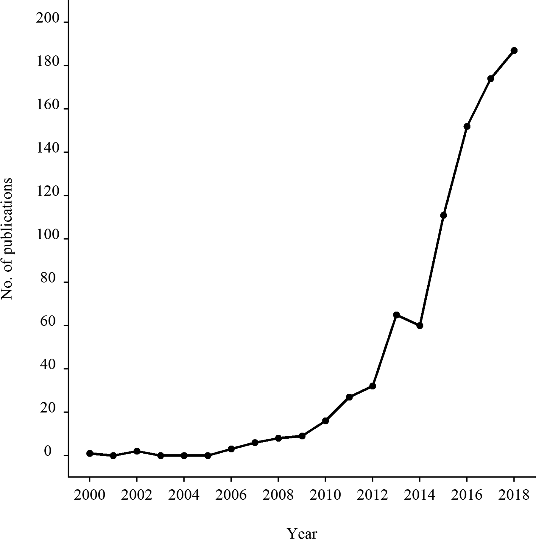
The number of publications from 2000 to 2018 that include “bifactor” in their titles or abstracts.

However, there are still several concerns to be addressed before embracing BiMs for studying the predictive validity of hierarchical constructs. First, the statistical performance of BiMs when used for prediction (e.g., bias, power, and Type I error rates) has not been examined via simulation. Importantly, several empirical studies have indicated that predictive BiMs seem to be subject to nonidentification problems (Chen et al., 2012; Chen, West, & Sousa, 2006; Eid et al., 2018). Second, because the true factor structure underlying empirical data is unobservable, researchers tend to adopt different models based on their conceptualizations of the hierarchical construct. Hence, BiM may not be the most appealing choice for researchers in every case. The practical consequences of adopting a different model to study the predictive validity of a BiM hierarchical construct remain unexplored. On the other hand, the consequences are also unknown when BiM is applied to a construct with a different latent structure (e.g., CFM or HOM). Given that “all models are wrong” (Box, 1976) for empirical data, is BiM a “more useful” model such that it is more likely to lead to the correct conclusion regardless of the true model?

The present study aims to address the two concerns via two Monte Carlo simulation studies. In Study 1, we examined the statistical performance of BiMs in various conditions. The augmented bifactor model (ABiM), which, as detailed in the following, is a more restricted variant of the bifactor-(S·I-1) model (Eid et al., 2017), was also introduced to solve the nonidentification problem. The effectiveness of the augmentation strategy was evaluated via a series of simulations. In Study 2, we investigated the practical consequences of adopting different models (BiM, HOM, and CFM) for constructs simulated with different factor structures. We examined estimation bias, power, and Type I error rate of each model when it was applied to different conceptualizations of hierarchical constructs to study predictive validity. The overall goal of the article is to provide readers with practical guidance on the use of predictive bifactor models in the context of study design, data analysis, and results interpretation. R code is also provided so that researchers can adapt it to gain a deeper understanding of the performance of BiMs in their own research contexts.

Bifactor Models

The underlying motivation of BiM is that each manifest indicator is directly influenced by three orthogonal components: the general factor, a specific factor, and item uniqueness. A graphical depiction of a classical bifactor measurement model is shown in Figure 2a. All indicators directly load on a single general factor that reflects the common variance running through them and a single specific factor that reflects the additional common variance shared among a cluster of items. Each specific factor—or “residualized factor”—is what is left among a cluster of indicators when the variance due to the general factor is removed (Reise, 2012). A mathematical representation of such multidimensionality is as follows:

Figure 2.

Graphic illustrations of (a) bifactor model, (b) augmented bifactor model, (c) bifactor-(S-1) model, (d) bifactor-(S·I -1) model, (e) correlated factors model, (f) higher-order factor model (f), and (g) augmented higher-order factor model.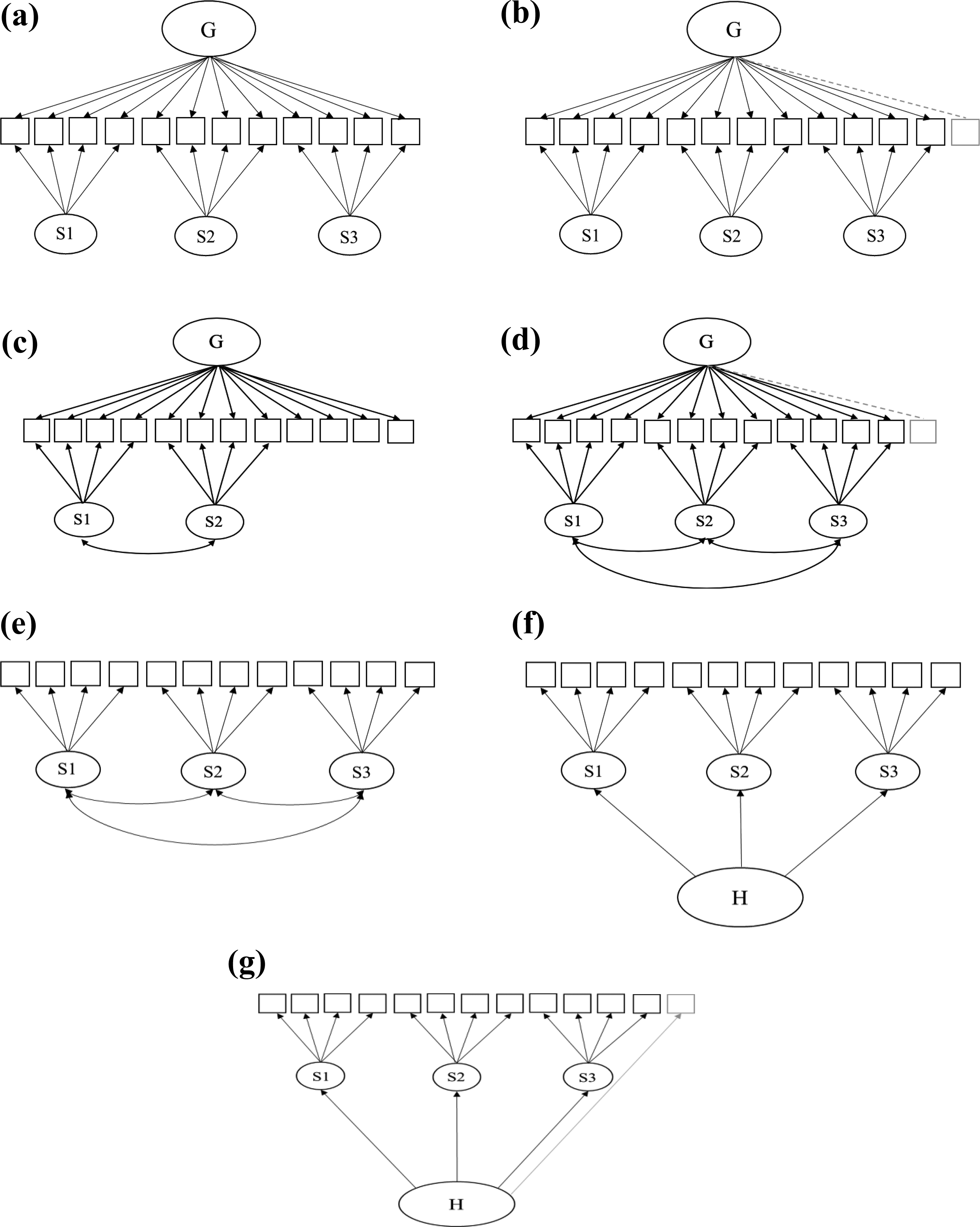

V a r (X_{i j}) = λ_{g i j}^{2} V a r (G) + λ_{s i j}^{2} V a r (S_{i}) + V a r (∊_{i j}) (1),

where Var(X_ij ) stands for the variance of observed scores of the jth item from the ith facet; Var(G) is the variance of the general factor (G); Var(S_i ) is the variance of the specific factor (S); Var(∊ _ij ) is the item-specific unique variance; and $λ_{g i j}$ and $λ_{s i j}$ are the factor loadings on the general factor and specific factor. Throughout this article, facet is used when referring to the latent construct that a subset of manifest indicators (single items or multiple-item composites) measure, and specific factor is used when referring to the residualized facet. Although different opinions exist regarding whether specific factors should be correlated (e.g., Jennrich & Bentler, 2012; Reise, 2012), we only focus on the classic BiM, where the general factor and all specific factors are orthogonal (Holzinger & Swineford, 1937). This model is attractive because it attributes shared variation across all manifest indicators to a general, overarching trait such as general intelligence, and additional covariation among a cluster of more highly correlated indicators (e.g., items assessing working memory) is attributed to a single specific factor so that researchers can directly evaluate the properties of each variance component.

The substantive meaning of residualized facets (e.g., What is working memory without general intelligence?) has been somewhat ambiguous. Gignac (2016) argued that the traditional conceptualization and measurement of facets (e.g., working memory) reflect a conglomeration of the general factor and a specific factor. It is the specific part instead of the common part that makes facets differentiable from each other. Therefore, we interpret specific factors as the pure facet without contamination from the general factor.

BiMs have a long but frequently underappreciated history. Holzinger and Swineford (1937) recognized their usefulness for representing the structure of hierarchical constructs and specifically, cognitive ability. However, the use of BiMs lain dormant for nearly 50 years (Reise, 2012). It was not until recent years that several articles have stoked researchers’ interest in BiMs (e.g., Chen et al., 2006, 2012; Reise, 2012; Reise, Moore, & Haviland, 2010; Reise, Morizot, & Hays, 2007). Methodological developments and their software implementation have further pushed these models toward the mainstream (Cai, 2010; Cai & Wirth, 2013; Cai, Yang, & Hansen, 2011; Chalmers, 2012; Gibbons et al., 2007; Gibbons & Hedeker, 1992; Jeon, Rijmen, & Rabe-Hesketh, 2014). There have been advances in exploratory bifactor models (Jennrich & Bentler, 2011, 2012) and two-tier bifactor models (Cai, 2010). However, we exclusively focus on confirmatory bifactor models with only one general factor because they are most commonly adopted.

Pros and Cons of Using BiM for Prediction

Predictive validity is fundamental to psychological research. Researchers invariably seek exogenous variables that can explain variance in important outcomes. When studying the predictive validity of hierarchical predictors, researchers are often interested in the incremental validity of a facet: Does it add explanatory power beyond that of the general factor? For example, researchers have started to explore the incremental validity of personality facets beyond the general domain factor (e.g., Aichholzer, Danner, & Rammstedt, 2018; Judge et al., 2013; McAbee, Oswald, & Connelly, 2014; Mike et al., 2018; Samuel & Widiger, 2008).

Intuitively, BiM is an excellent vehicle for studying the predictive validity of hierarchical constructs because the general factor in Figure 2a can be conceived as the broad construct, and the differentiated subdomains are treated as the specific factors. Therefore, BiMs possess the conceptual attractiveness of separating the general factor and specific factors and modeling them as latent variables, which allows direct examination of their independent relationships with outcomes. The outcome variable can be regressed on the general factor and all specific factors via a general structural equation model (SEM). Standardized regression coefficients in such bifactor predictive models can be interpreted as showing the unique contribution of each factor to the outcome variable(s) independent of other factors due to the orthogonality of the factors (Reise et al., 2013). In fact, Gustafsson and Balke (1993) realized this conceptual advantage and used BiM for prediction more than two decades ago.

A major problem of BiM is nonidentification when applied for prediction purpose. Chen and colleagues (2006) were the first to note that analyses with BiM may be nonidentified when all specific factors are included with the general factor in the prediction of outcome variable(s) even if the measurement model appears satisfactory. The nonidentification problem may show up in the form of abnormally large regression coefficients and huge standard errors, negative residual variances of outcome variables, or nonconvergence (Eid et al., 2018). Eid and colleagues (2018) clarified that such bifactor predictive models are nonidentified when the factor loadings of the manifest indicators on the general factor are the same and there are only two indicators per specific factor. We further note that nonidentification can occur when loading patterns follow the proportionality constraint because of exact linear dependency between the general factor and all specific factors (Mansolf & Reise, 2016; Schmid & Leiman, 1957; Yung, Thissen, & McLeod, 1999). The proportionality constraint refers to the condition where the ratio between $λ_{g i j}$ and $λ_{s i j}$ is a constant for items within a single facet (this constant can be different across facets; Reise, 2012). If factor loadings on the general factor are not identical or the proportionality constraint is not exactly satisfied, in principle, the general factor and all specific factors can be included to predict outcome variable(s) simultaneously because the model is mathematically identified. In practice, we speculate that problems are more likely to arise as factor loadings approximate proportionality or factor loadings on the general factor become more similar to each other, which is known as empirical underidentification (Rindskopf, 1984). As one reviewer noted, proportionality is one of the best hierarchical structures one could expect because all facets are measured distinctly. However, predictive BiM is not identified in the ideal condition, which is an important limitation.

Strategies to Mitigate the Nonidentification Problem of BiM

Several strategies have been proposed to reduce the nonidentification problem by focusing on circumventing or eliminating linear dependency. A first strategy was proposed by Chen and colleagues (2006). They suggested fixing the regression coefficient(s) of at least one specific factor to zero and freely estimating the remaining ones. Because only a subset of predictors is included in the prediction of an external variable, linear dependency among predictors is mitigated. This strategy is limited in that (a) which specific factor to exclude is arbitrary, (b) the impact of excluding some specific factor on the estimation of regression coefficients of the other factors is unknown, and (c) researchers are unable to test the incremental validity of all specific factors simultaneously. A second strategy was proposed by Eid and colleagues (2018). It focused on eliminating linear dependency among predictors by selecting a reference facet (or indicator) and forcing indicators of this facet to load only on the general factor. Because only a subset of indicators is allowed to load on a specific factor, there is no longer linear dependency among predictors. This strategy is preferable to the first one because it not only eliminates the linear dependency problem but also gives a clear meaning to the general factor (see Eid et al., 2017, for formal proof). However, it is also limited in some ways. First, similar to Chen and colleagues’ strategy, the selection of the reference facet is somewhat arbitrary. Second, the “general factor” is no longer the broad construct that a measure was designed to capture. It now confounds the meaning of the reference facet with the general factor. If different facets/indicators are chosen, the construct validity of all factors may change subsequently. Third, specific factors no longer represent what is left after controlling for the broad trait. Instead, they are residualized facets after controlling for the reference facet. To circumvent the problem that a general factor equals a facet and cannot be interpreted as the broad construct, Eid et al. (2017) recommended that researchers assess the general factor directly by appropriate indicators that are not related to a specific domain.

We followed Eid et al.’s (2017) recommendation to measure the general factor directly and adopted a modified strategy that also focuses on eliminating linear dependency, but it avoids the drawbacks of current approaches. Instead of fixing some regression coefficients or arbitrarily choosing a reference facet, we suggest adding a new indicator that principally taps the general factor. This new indicator should be specified as loading only on the general factor while the loadings of the original items are unchanged (see Figure 2b). As the new indicator only loads on the general factor and does not load on any specific factor, the (approximate) linear dependency between the general factor and all specific factors is eliminated.² Castro-Schilo, Grimm, and Widaman (2016) used a similar strategy to improve the identification of correlated trait-correlated method models and found that it worked well. Statistically speaking, the modified strategy is a specific variant of the bifactor-(S·I-1) model (see Figure 2d) because the modified strategy specifies that all specific factors are orthogonal to each other while the bifactor-(S·I-1) model allows correlated specific factors. If researchers used more than one indicator to measure the general factor, then ABiM is a specific variant of the bifactor-(S-1) model (Eid et al., 2017; see Figure 2c). In the present study, we only focus on one indicator.

It is often easy to create the type of indicator we propose. For instance, researchers could write items like “I am an extraverted person” to assess the broad construct Extraversion. Researchers should choose items that are as general as possible. Statements like “I am an outgoing person” or “I am an assertive person” may not be good examples because they also tap other facets such as Sociability and Assertiveness. For the sake of clarity, we label the modified bifactor model as the augmented bifactor model. Compared to the earlier two approaches, the augmentation strategy allows examination of the unique contribution of all specific factors simultaneously while at the same time keeping the construct validity of the general factor intact or even enhancing it, thus potentially solving both the conceptual and statistical problems of BiM.

Correlated-Factors Model and Higher-Order Factor Model

Before the renaissance of BiM, the CFM (see Figure 2e) and the HOM (see Figure 2f) were the dominant models for hierarchical constructs (Brunner, Nagy, & Wilhelm, 2012). In CFM, indicators from a facet load on their corresponding latent factors and latent correlations among these first-order factors are freely estimated. The HOM can be seen as an extension of the CFM in that a higher-order factor is further extracted from the correlation matrix of the latent first-order factors, thus directly mapping to the “hierarchical” nature of focal constructs.

Conceptually, CFM is very different from BiM and HOM because there is no hierarchy differentiation. The first-order factors in CFM represent an amalgamation of the general factor and specific factors when applied to hierarchal constructs (Brunner et al., 2012; Murray & Johnson, 2013). HOM, on the other hand, shares some commonalities with BiM. Both models aim to represent the construct hierarchy in its entirety by modeling latent constructs at different levels of generality. The higher-order factor in HOM conceptually resembles the general factor in BiM, reflecting the common variance running through all observed indicators. The first-order factor residuals in HOM are analogous to the specific factors in BiM, which can be considered as unambiguous representations of the unique components of facets (Gignac, 2009). BiM and HOM differ in how levels of abstraction are modeled (Markon, 2019). In BiM, the general factor is at a higher level of abstraction because it directly influences a greater breadth of observed indicators. In HOM, the higher-order factor reflects a higher level of abstraction because it influences first-order factors and exerts its influence on observed indicators only through first-order factors. Users of HOM have often focused on the higher-order factor and paid less attention to properties of first-order factor residuals.

Statistically, the three types of models are closely related. The relationship between CFM and BiM is complex (Asparouhov & Muthén, 2019). When the number of facets is two or three, CFM is nested within BiM. When the number of facets is equal to or greater than four, the two models are not nested (but can be statistically equivalent; Asparouhov & Muthén, 2019). Regarding the relationship between HOM and BiM, it is well known that HOM is a restricted case of BiM with proportionality constraints (Reise, 2012; Yung et al., 1999). Thus, BiM is a more flexible representation of hierarchical constructs than HOM.

When CFM is used for prediction, the outcome variable is regressed on all first-order factors simultaneously. However, CFM-based regression may not be ideal for examining the predictive validity of hierarchical constructs. First, this approach precludes the examination of the predictive validity of the general factor because it is omitted from the model. Second, depending on the degree of multicollinearity, parameter estimation bias and Type I error rate may suffer (Grewal, Cote, & Baumgartner, 2004). Thus, CFM may not be appropriate for studying the predictive validity of hierarchical constructs for both conceptual and statistical reasons. However, we included CFM in Study 2 to better understand its characteristics.

Given the similarity between HOM and BiM, HOM seems a good alternative. Conceptually, researchers can regress the outcome variable on the higher-order factor and all first-order factor residuals simultaneously. As the higher-order factor and all residuals of first-order factors are orthogonal to each other, regression coefficients can be interpreted as independent contributions. However, simultaneous estimation of such a model is not identified due to the exact linear dependency between the higher-order factor and all first-order factor residuals (Brunner et al., 2012; Mansolf & Reise, 2016; Schmiedek & Li, 2004). Alternatives have been proposed within the framework of HOM to circumvent the problem of nonidentification by arbitrarily fixing some paths (Christensen et al., 2001; Salthouse, 1998). However, these alternatives have been shown to run the risk of inflating the predictive validity of the high-order factor with downward bias in the predictive validity of specific factors (Schmiedek & Li, 2004).

The Present Study

Two Monte Carlo simulation studies were conducted to examine the performance of BiM for prediction. Study 1 aimed to (a) systematically evaluate the statistical performance of BiM (probability of anomaly, estimation bias, the power, and Type I error of the regression coefficients) and (b) examine the effectiveness of ABiM in reducing anomalies and improving power, holding Type I error rate constant, and reducing estimation bias in predictive models. Study 2 was designed to compare the performance of BiM with CFM and HOM when used for prediction. Specifically, we examined whether BiM is more flexible than the other two models; that is, does BiM exhibit superior performance to the other two models when it is applied to a construct that is inherently inconsistent with the model specifications?

Study 1

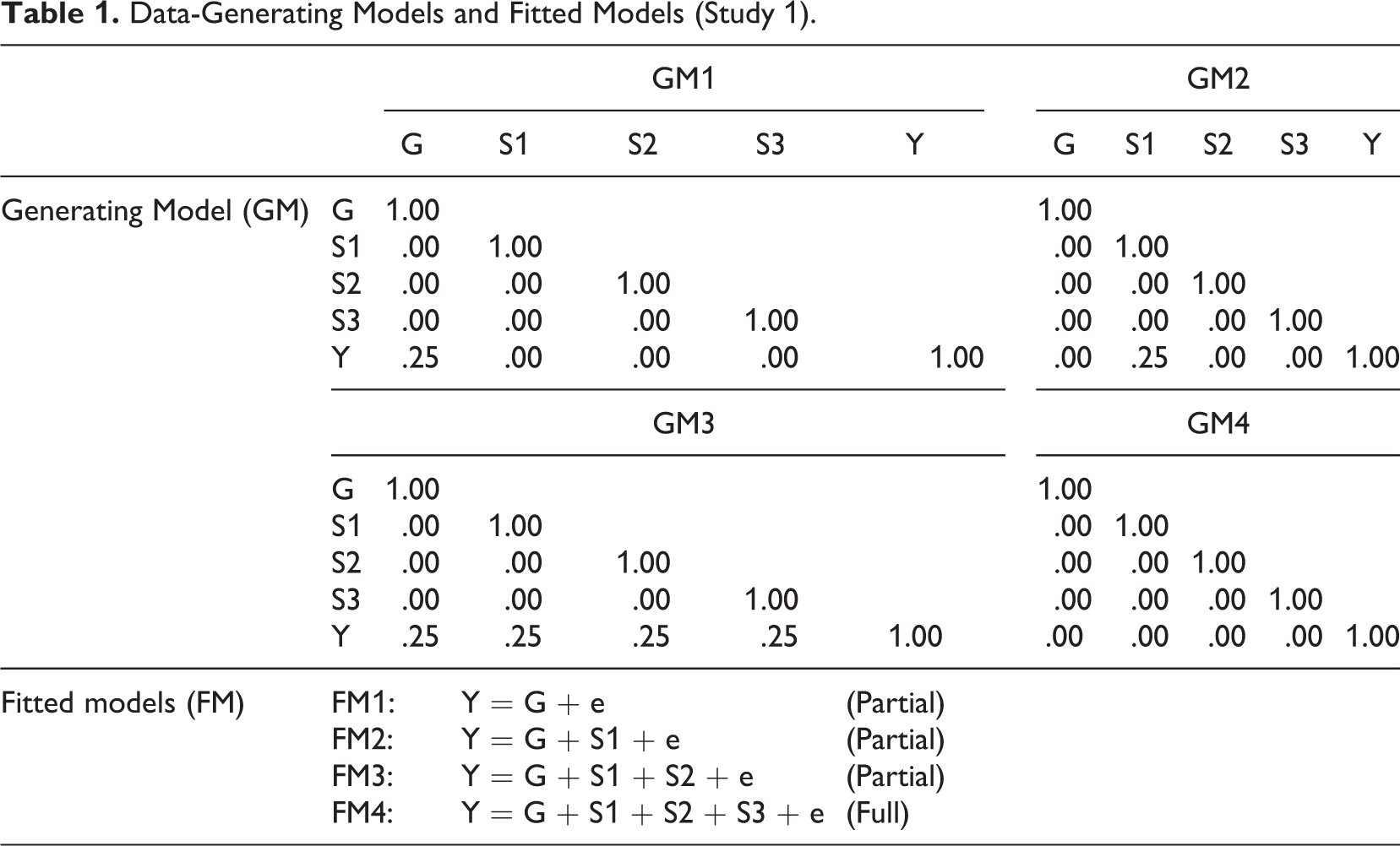
Preliminary simulations showed that the number of facets did not have a substantial impact on key results. We therefore fixed the number of facets to three throughout the study for the sake of simplicity. Moreover, three facets are common for many widely used scales, such as the Maslach Burnout Inventory (Maslach, Jackson, & Leiter, 1996), the Utrecht Work Engagement Scale (Schaufeli, & Bakker, 2003), and the Big Five Inventory-2 (Soto & John, 2017). As shown in Table 1, four matrices representing correlation patterns among predictors (i.e., a general factor and three specific factors) and the outcome variable that are likely to be encountered in real-world settings were used as data generating models (GM1-GM4). GM1 simulates conditions where only the general factor predicts the outcome. We use this condition because several studies have shown that the general ability factor is the only factor that matters when predicting various job outcomes. In particular, it has been argued that specific abilities do not matter, or the so-called not-much-more-than-g phenomenon (e.g., Olea & Ree, 1994; Ree & Earles, 1991; Ree et al., 1994). GM2 stands for cases where only one specific factor is predictive of outcomes. This condition has its roots in Mike et al. (2018), where they reported that the general Openness factor was not predictive of the obsessive-compulsory personality disorder but the Action and Fantasy facets were. GM3 stands for a case where all factors have unique contribution. GM4 is the dreaded “null hypothesis is true” case, where neither the general factor nor any of the specific factors predict the outcome. Although not reported often (maybe because it is hard to publish null results), this condition can at least serve as a baseline. Importantly, we tried sampling diverse conditions. Therefore, we included both typical and less typical conditions. All nonzero correlations (equivalent to beta coefficients due to orthogonality among predictors) were fixed to .25, which represents a moderate but frequently encountered predictive validity in organizational research. For example, Bosco et al. (2015) extracted 147,328 correlations from studies published in Journal of Applied Psychology and Personnel Psychology from 1980 to 2010. They found that the average correlations in 20 domains of mainstream organizational research ranged from .107 to .342, with an overall mean correlation of .22, which is also very close to the average correlation from 25,000 social psychology studies (r = .21; Richard, Bond, & Stokes-Zoota, 2003).

Table 1.

Data-Generating Models and Fitted Models (Study 1).

		GM1					GM2
		G	S1	S2	S3	Y	G	S1	S2	S3	Y
Generating Model (GM)	G	1.00					1.00
	S1	.00	1.00				.00	1.00
	S2	.00	.00	1.00			.00	.00	1.00
	S3	.00	.00	.00	1.00		.00	.00	.00	1.00
	Y	.25	.00	.00	.00	1.00	.00	.25	.00	.00	1.00
		GM3					GM4
	G	1.00					1.00
	S1	.00	1.00				.00	1.00
	S2	.00	.00	1.00			.00	.00	1.00
	S3	.00	.00	.00	1.00		.00	.00	.00	1.00
	Y	.25	.25	.25	.25	1.00	.00	.00	.00	.00	1.00
Fitted models (FM)	FM1:		Y = G + e			(Partial)
	FM2:		Y = G + S1 + e			(Partial)
	FM3:		Y = G + S1 + S2 + e			(Partial)
	FM4:		Y = G + S1 + S2 + S3 + e			(Full)

Data generation and model estimation

We also manipulated the following factors to evaluate the performance of augmented bifactor predictive models: (a) loadings on the general factor (LG): .40 and .60; (b) loadings of the additional indicator on the general factor (LG1): .40 and .60; (c) loadings on specific factors (LS): .40 and .60; (d): whether the augmented bifactor model was used or not (augmented); (d) the number of indicators per facet (indicators): 4 and 8; and (f) sample size (SS): 200 to 800 with increments of 100. Finally, we fitted four different models to each generated data set to mimic strategies researchers are likely to adopt in realistic situations. For example, some researchers are only interested in the general factor. Therefore, they would regress outcome variables only on the general factor and omit all specific factors from the regression equation; this is Fitted Model 1 (FM1). Other researchers might be interested in the general factor and do not mind exploring the effects of specific factors. They might also be aware of the strategy suggested by Chen and colleagues (2006). Therefore, they would regress outcome variables on the general factor and some of the specific factors. FM2 using one specific factor and FM3 using two specific factors represent strategies that are likely to be adopted by these researchers. Many users of bifactor predictive models are simultaneously interested in the effects of the general factor and all specific factors and would include all factors in the model when predicting external variables (e.g., Chen et al., 2012, 2013; Debusscher, Hofmans, & De Fruyt, 2017; McAbee et al., 2014; Moshagen, Hilbig, & Zettler, 2018), which is FM4. FM1, FM2, and FM3 were labeled as partial models because only a subset of specific factors was included in the prediction, and FM4 was labeled as the full model because all the factors were used in the regression.

In total, there were 3,584 conditions (4 × 2 × 2 × 2 × 2 × 2 × 7 × 4 = 3,584). To achieve better representation of realistic situations and increase the generalizability of our findings, factor loadings within each replication were randomly drawn from a uniform distribution U (L – .10, L + .10), where L is the prespecified loading for that condition. Adopting .20 as the range for the uniform distribution is intended to represent realistically satisfactory bifactor structures where loadings on the same factor should have a similar size despite some variability. If loadings on the same factor vary greatly (e.g., from .20 to .80), one might question the appropriateness of the bifactor model. But we note that the choice of range may influence results given that a wider range should result in a lower probability of empirical underidentification. The outcome variable was set to be a single manifest variable. Population correlation matrices were generated using

\sum = Λ Φ Λ' + Θ (2)

where Λ is the factor loading matrix (including the outcome variable whose loading on its factor was set to 1), Φ is the latent factor correlation matrix (those shown in Table 1), and Θ is the diagonal error variance-covariance matrix scaled to ensure the diagonal elements of Σ equal 1 (fixing all factor variance to 1). Individual-level sample data were generated from the population matrices using the psych R package (Revelle, 2018). Each simulated sample data set was fitted by models FM1 through FM4 using the R package lavaan (Rosseel, 2012). Maximum likelihood estimation was used. When software reported any anomalous result (e.g., nonconvergence, negative variance, or nonpositive definite residual correlation matrix) for a replication, it was rejected, and another draw was taken until 1,000 valid replications were obtained. The number of anomalous replications was recorded for each condition. All indices detailed in the following were calculated from valid replications. This strategy ensures that comparisons between conditions are based on the same number of valid replications so that the influence of sampling variability is held constant (Castro-Schilo et al., 2016) while simultaneously we can assess the likelihood of problematic solutions. The R package SimDesign was used to streamline the simulation process (Sigal & Chalmers, 2016). R script and results can be found on the Open Science Framework website (https://osf.io/kjt5m).

Analysis

Our primary interest in the present study was the four beta coefficients that represent the predictive validity of the general factor and the three specific factors. We focused on four criteria when evaluating the performance of traditional bifactor predictive models and augmented bifactor predictive models: (a) the frequency of anomalous results, (b) power/Type I error rate for hypothesis tests about the regression coefficients, (c) bias of regression coefficients, and (d) root mean square error (RMSE) of regression coefficients. Any replication reporting errors or warnings like nonconvergence, nonidentification, negative variance, and nonpositive definite residual matrix was considered an anomaly. We used the anomaly rate (AR) to index the frequency of estimation problems, calculated as follows:

A R = \frac{No . of Anomalies}{1000+No . of Anomalies}

Power was defined as the proportion of replications where a true nonzero effect was correctly detected, and the Type I error rate was defined as the proportion of replications where a true zero effect was falsely found to be significant. Bias was calculated as the difference between the average value of the estimate and the true parameter. Positive bias indicates overestimation, and negative bias indicates underestimation. Bias that falls between –10% and 10% of the true value is often considered acceptable (Muthén & Muthén, 2002). RMSE is given by the square root of the average of the squared difference between the estimated and true parameter. RMSE is an index of overall accuracy that combines bias and sampling variability. Note that although there are three specific factors in our models, when more than one specific factor was included in the regression, we only report power/Type I error rate for the first specific factor because the pattern was almost identical across specific factors.

Results

We discuss anomaly rate, power, and Type I error rate in separate sections. Power and Type I error rate associated with the general factor and specific factors are also presented separately. Anomaly rate, power, Type I error rate, estimation bias, and RMSE for each condition are available on request. Figures for power/Type I error and bias are shown in the following, and results for RMSE can be found on the Open Science Framework website. In addition, given that the results between the three partial models (FM1-FM3) were very similar to each other in most cases, we only report results averaged across the three partial models and compare them with results from FM4. More detailed results for each fitted model are presented in Appendices A through F.

Anomaly rate

Frequent anomalous results were observed in some conditions. For example, the AR was sometimes greater than .40 when the classic bifactor model (FM4) was fitted to the data in small samples. To provide a precise estimate of the influence of different simulation factors and their interactions, we computed an eight-factor analysis of variance (ANOVA) with the AR as the dependent variable. All main effects and two-way interactions were included in the model. This model explained 86.5% of the total variance in AR. We report predictors that explained at least 2% of the total variance. The strongest main effect was observed for sample size (η² = .205), followed by the fitted model (η² = .095), the type of bifactor model used (BiM vs. ABiM; η² = .073), number of indicators per facet (η² = .051), the magnitude of factor loadings on the general factor (η² = .040), and the magnitude of factor loadings on specific factors (η² = .032). The effect of data-generating model and the magnitude of factor loading of the extra indicator on the general factor had negligible effect on the AR (η²s < .01). Several interactions were also substantial. Specifically, sample size interacted significantly with the type of bifactor model used (η² = .041), fitted model (η² = .026), factor loadings on the general factor (η² = .047), number of indicators per facet (η² = .058), and factor loadings on specific factors (η² = .032). The fitted model also interacted significantly with the type of bifactor model used (η² = .022).

Figure 3 provides a visualization of the relationship between the AR and different factors. When both the general factor and all specific factors were used to predict the outcome, researchers are very likely to encounter anomalous results, especially when sample size is small and loadings on the general factor are relatively low. When loadings on the general factor were .40 and the number of indicators per facet was four, the anomaly rate exceeded 10% for all sample sizes less than 700 and was almost 35% for samples of 200. Augmenting traditional bifactor models with just one more indicator greatly reduced the rate of anomalous results. For example, when the sample size was 200, the number of indicators per facet was four, and average loading on the general factor was .40, adding one more indicator reduced the anomaly rate from nearly 35% to about 10%. When the sample size reached 300, the anomaly rate dropped below 5%. The same pattern held in other less extreme conditions.

Figure 3.

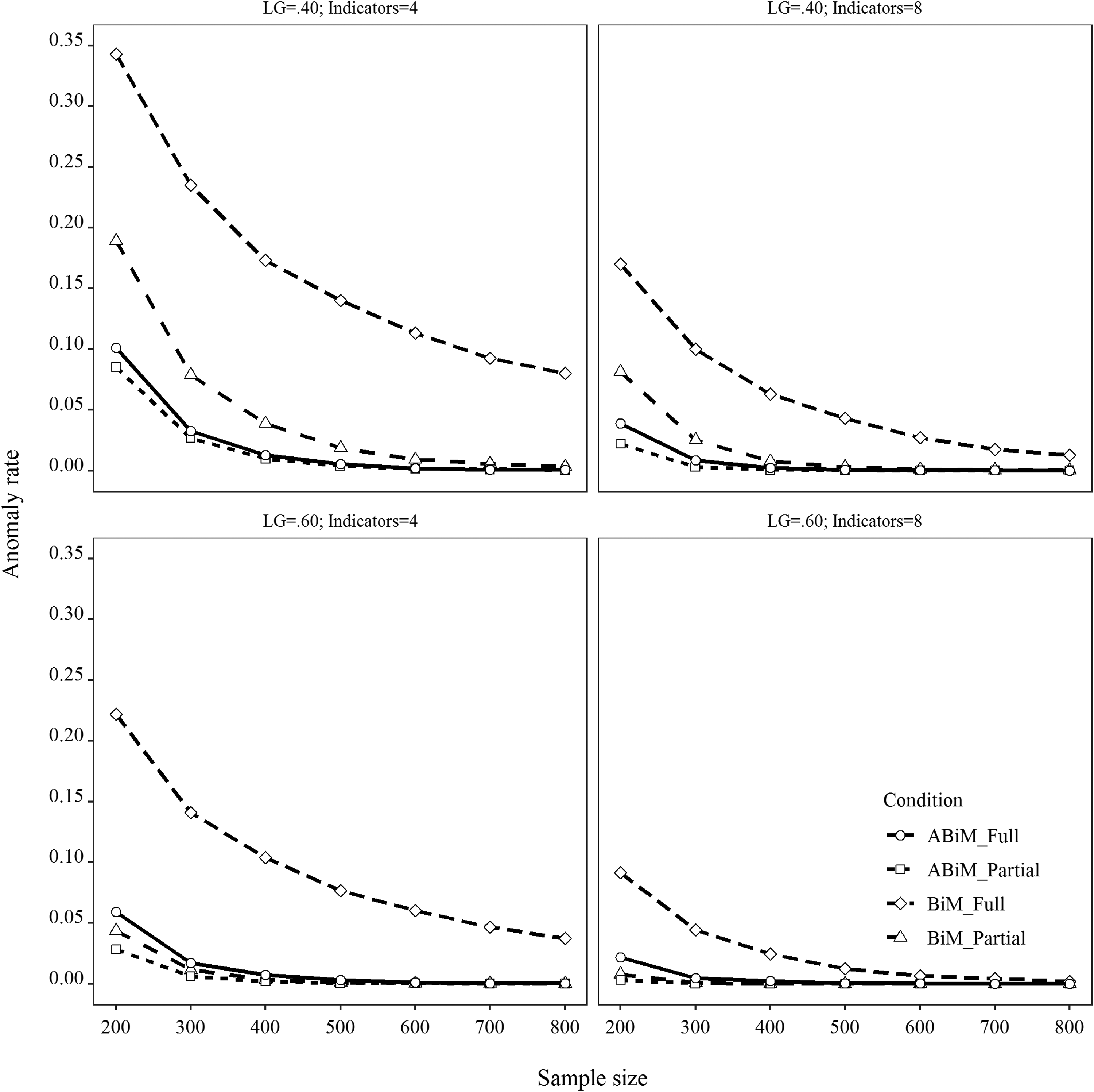
Anomaly rate in different conditions. LG = loadings on the general factor; indicators = number of indicators per facet; ABiM = augmented bifactor model; BiM = bifactor model; full = full predictive model (FM4); partial = partial predictive model (FM1-FM3).

Given the general statistic dictum that a greater number of parameters generally makes model estimation harder when sample size is held constant, it is surprising that increasing the number of indicators per facet ameliorated the anomaly problem (but see Idaszak, Bottom, & Drasgow, 1988, who found improved results for factor analysis when increasing the number of indicators per factor). For example, when we held the sample size to 200 and average loadings on the general factor to .40 and BiM was used, the anomaly rate was close to 35% when the number of indicators per facet was four. It was 17% when the number of indicators per facet was doubled. When the average loading on the general factor was .60, the same pattern was observed: The AR dropped from about 23% to 10% when number of indicators per facet was doubled. In the best condition where ABiM was used (average loading on the general factor was .60, and number of indictors per facet was eight), the anomaly rate was 2% even when sample size was only 200.

Power, bias, RMSE

General factor

The first column of Figure 4 shows results for the conditions where only the general factor predicted the outcome variable in the population (GM1). The three partial models had power greater than .80 even when the sample size was only 200. Furthermore, Figure 5 shows estimation of the regression coefficient for the general factor was virtually unbiased. When the full model FM4 was fitted, power patterns differed substantially from the three partial models. Specifically, when the classic bifactor model with four indicators per facet was fitted, power was below .50 for the sample size of 200 and remained below .80 even when the sample size was 800. For the augmented bifactor models, power reached .80 for samples of 400. For eight indicators per facet, samples of 300 sufficed to reach the .80 power level. More importantly, the additional power of the augmented model came without increased bias. In fact, the augmented model stabilized parameter estimates, as demonstrated by the shrinking RMSEs in the first column of Appendix C.

Figure 4.

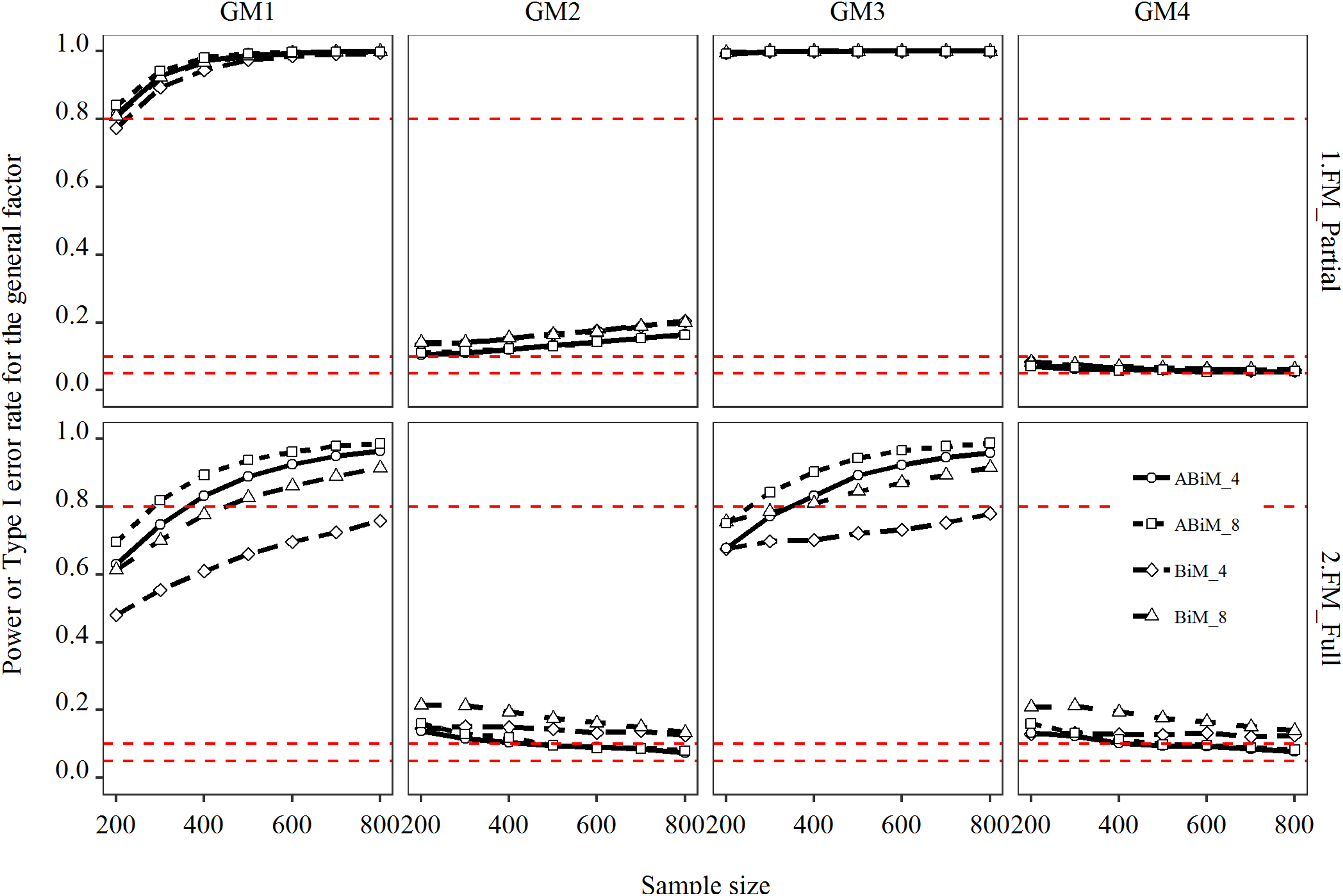
Power or Type I error rate for the general factor. Columns 1 and 3 represent power under different conditions. Columns 2 and 4 stand for Type I error rate in different conditions. GM = generating model; FM = fitted model; ABiM = augmented bifactor model; BiM = bifactor model; full = full predictive model (FM4); partial = partial predictive model (FM1-FM3). The number following ABiM or BiM indicates number of indicators per facet. The three red dashed lines correspond to y values of .05, .10, and .8.

Figure 5.

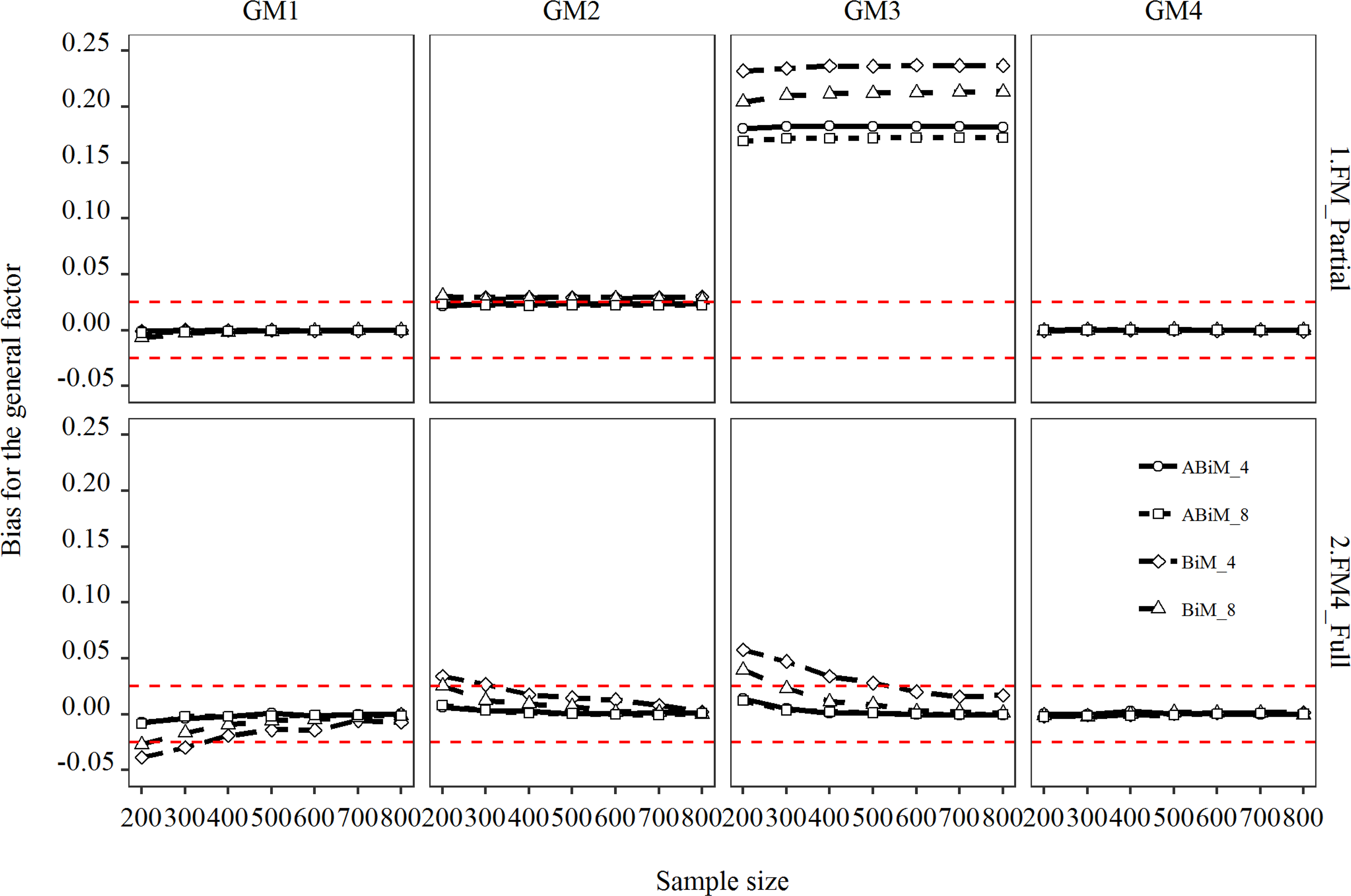
Bias for the general factor. GM = generating model; FM = fitted model; ABiM = augmented bifactor model; BiM = bifactor model. The number following ABiM or BiM indicates number of indicators per facet. Full = full predictive model (FM4); partial = partial predictive model (FM1-FM3). The three red dashed lines correspond to y values of –.025 and .025, which reflected 10% relative bias.

When the general factor and all three specific factors were predictive of the outcome (GM3), the three partial models (FM1-FM3) had almost perfect power for the regression coefficient of the general factor. However, these high levels of power were obtained at the cost of severely overestimating this regression coefficient. As can be seen in the third column of Figure 5, regardless of sample size, even the lowest bias was higher than .125 (50% relative bias) for the three partial models. Apparently, the predictive validity of the omitted specific factors was shifted onto the general factor. The more variables omitted, the more serious the overestimation (as can be seen in the third column of Appendix B). Interestingly, the ABiM reduced the degree of overestimation by about 20%. The severe bias of estimates of the regression coefficient of the general factor was almost entirely eliminated when the fitted model FM4 matched the generating model GM3. But power was reduced: More than 800 respondents would be required to obtain power of .80 when the classic bifactor model with four indicators per facet was used. For the augmented model, 400 respondents sufficed to obtain power above .80. If the number of indicators per facet were doubled, only 300 respondents were needed.

Specific factors

As can be seen from the second column of Figure 6, when only one of the specific factors was predictive (GM2), fitting the partial models produced power higher than .80 as long as sample size exceeded 300, regardless of whether the classic or augmented bifactor model was used. Moreover, Figure 7 shows that bias was close to zero across conditions. However, when the full model FM4 was fitted, power was reduced; the classic model with four indicators per facet never reached a power of .80 when sample size was equal to or below 800. Moreover, Appendix F shows that RMSE increased substantially compared to when the partial models were fitted, indicating more volatile parameter estimates. Fortunately, the augmented model reduced the minimal sample size required for a power of .80 to 400. When the number of indicators per facet was doubled, only 300 respondents were sufficient. As displayed in Figure 7, bias stayed within the acceptable range, and the RMSEs of FM4 stayed close to those of the partial models when the augmented model was fitted.

Figure 6.

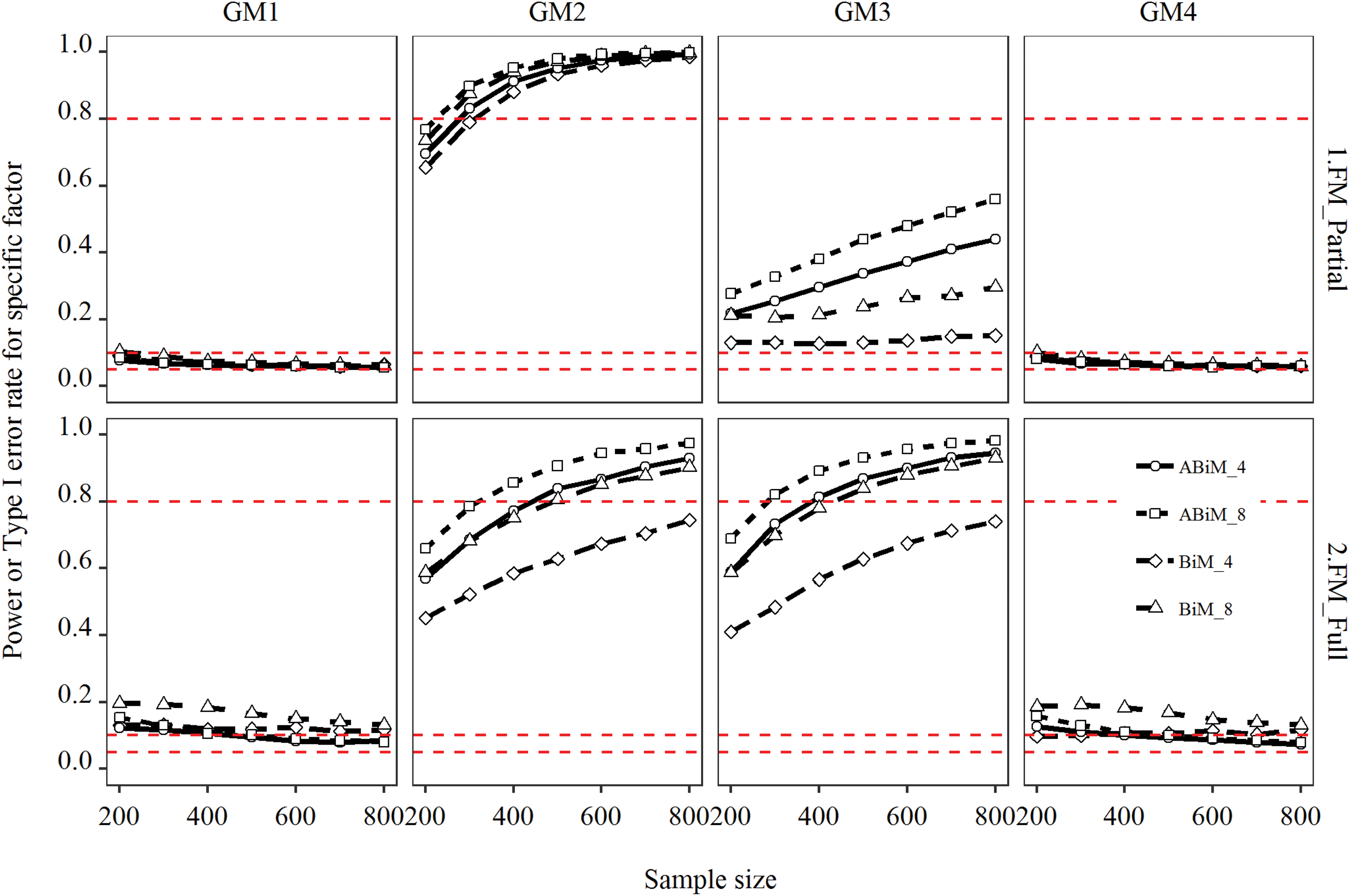
Power or Type I error rate for specific factor. Columns 2 and 3 represent power under different conditions. Columns 1 and 4 stand for Type I error rate in different conditions. GM = generating model; FM = fitted model; ABiM = augmented bifactor model; BiM = bifactor model; full = full predictive model (FM4); partial = partial predictive model (FM2-FM3). The number following ABiM or BiM indicates number of indicators per facet. The three red dashed lines correspond to y values of .05, .10, and .8.

Figure 7.

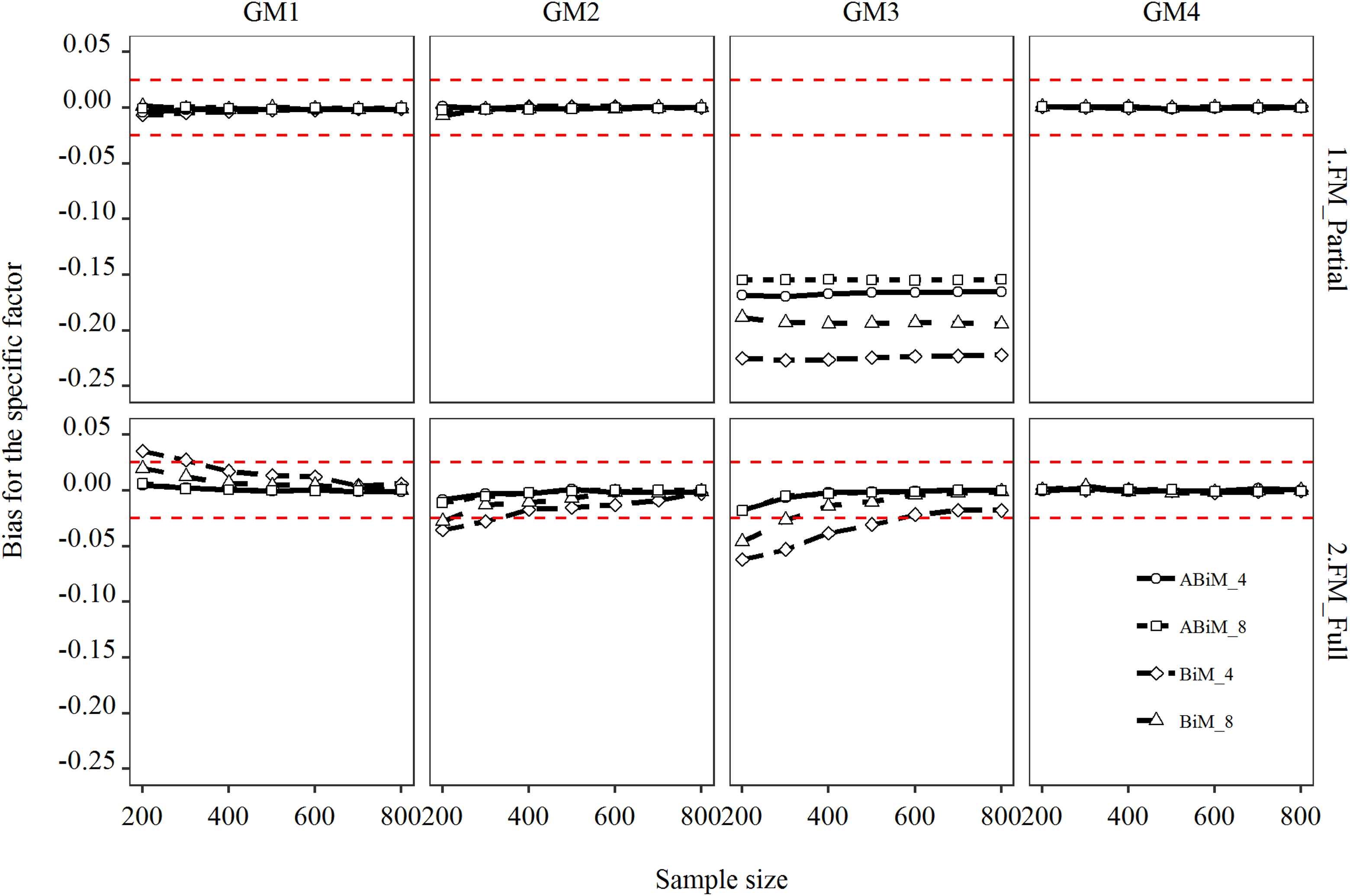
Bias for the first specific factor. GM = generating model; FM = fitted model; ABiM = augmented bifactor model; BiM = bifactor model; full = full predictive model (FM4); partial = partial predictive model (FM2-FM3). The number following ABiM or BiM indicates number of items per facet. The three red dashed lines correspond to y values of –.025, and .025, which reflected 10% relative bias.

When the general factor and all specific factors were nonzero predictors (GM3), fitting the two partial models greatly affected power, as shown in the third column of Figure 6. When the classic bifactor model with four indicators per facet was used, the power to detect the nonzero regression coefficient of the first specific factor was below 35% even in a condition (not shown) with N = 2,000. The augmented model increased power substantially over the classic model. Consistent with previous findings, doubling the number of indictors also increased power. The third column of Figure 7 shows severe bias in estimates of the regression coefficient of the specific factor when the two partial models (FM2 and FM3) were fitted. Bias was almost –.25 for the classic model with four indicators per facet. The reason why the augmented model and increased number of indicators per facet increase power is that they reduce the degree of underestimation and sampling variability simultaneously, as shown in the third columns of Figure 7 and Appendix F. When the full model FM4 was fitted, the pattern was nearly identical to what we reported in the previous paragraph. Augmenting one more indicator effectively reduced the minimal sample size required for power of .80 to 400. Further doubling the number of indicators reduced it to 300. Bias still stayed within the acceptable range. RMSE was also within the normal range.

Type I error rate, bias, and RMSE

General factor

When only the first specific factor was predictive of the outcome (GM2), fitting FM1 resulted in unacceptably high Type I error rates. As shown in the second column of Figure 4, Type I error rates were always greater than 10%. A closer inspection of Appendix A revealed that this pattern was solely driven by FM1 given that the Type I error rate increased nearly linearly with sample size in FM1. When the classic model with four indicators per facet was used, the lowest Type I error rate was more than 20%. Doubling the number of indictors per facet was of little value. The augmented model reduced the Type I error rate slightly, but it was still too high to be acceptable. These high Type I error rates result from overestimation of the regression coefficient for the general factor (it was 0 in GM2). As can be seen in the second column of Appendix B, bias was around .0875 (35% of .25) across sample sizes when the classic model was used. It dropped to around .065 (26% of .25) for the augmented model. When FM2 and FM3 were fitted, the Type I error rates were close to .05. There were little substantial differences between the classic and augmented models in these two conditions. The general pattern when FM4 was fitted was very similar except that Type I error rates were slightly higher when the sample sizes were below 400. Bias and RMSE for FM2, FM3, and FM4 stayed within the acceptable range across conditions.

When neither the general factor nor any of the specific factors was predictive (GM4), fitting the three partial models resulted in no inflation of Type I error rates, bias, and RMSE across conditions. The pattern of fitting FM4 was almost identical to what we found when GM2 was the data-generating model. Type I error rate was below .10 for samples of 400 or more and close to .05 for the sample size of 800. Bias and RMSE for FM4 stayed within the acceptable range across conditions.

Specific factors

As can be seen from the first and the last columns of Figures 6 and 7, the pattern for GM1 and GM4 was almost identical. Fitting the two partial models (FM2 and FM3) did not result in unacceptably high Type I error rates. As long as the sample size exceeded 300, Type I error rates were under .10 regardless of whether the classic or augmented model was used. As the sample size increased to 800, Type I error rates converged to .05. Bias and RMSE were both within the acceptable range across conditions. When the full model FM4 was fitted, results were somewhat different. When the sample size was 200, Type I error rates reached .20. Even for the augmented model, the Type I error rate was above .10. Additional analyses indicated that samples in excess of 1,000 would be needed to keep Type I error rates of the classic model under .10. Fortunately, only 500 respondents were needed to keep the Type I error rate under .10 for the augmented model. Bias and RMSE were within the acceptable range across conditions.

Discussion

To our knowledge, this is the first simulation study that examined the prevalence of anomalous results in bifactor predictive models, factors that influenced their probabilities, and the effectiveness of a new strategy to reduce anomalous results (Eid and colleagues did not use simulation to examine the performance of their methods). Based on a series of simulations, we found that anomalous results are most likely to occur when the general factor and all specific factors are included in the prediction of an external variable, sample size is small, factor loadings are modest, and only a small number of indicators per facet are available. Although fixing the path from one or more specific factors to outcomes to zero can reduce the occurrence of anomalous results, this practice led to high upward bias for the predictive validity of general factor and downward bias for specific factors in many cases. We also provide initial examinations of the power, Type I error rate, and estimation accuracy of regression coefficients in bifactor predictive models. It was found that regression coefficients can be severely biased and unstable under some circumstances, resulting in low power and high Type I error rates.

Researchers should be aware of anomalies of classic bifactor predictive models because unsatisfactory results may be obtained even if the measurement model is well identified. When the population factor loading matrix does not satisfy exact proportionality constraints (which means that the population model is identified), classical bifactor predictive models that include all specific factors with the general factor may still have estimation problems, particularly when sample size is small. Increasing sample size can decrease anomaly rates because more observations reduce sampling fluctuations, thus facilitating empirical identification and convergence to proper solutions (Anderson & Gerbing, 1984; Boomsma, 1985; Chen et al., 2001; Rindskopf, 1984). Consistent with some previous findings (Anderson & Gerbing, 1984; Idaszak et al., 1988), given a fixed sample size, increasing the number of indicators per facet can also help to reduce the anomaly rate. Apparently, more indicators per facet yields a lower probability of data that approximately satisfies the proportionality constraint or factor loadings, thus improving empirical identification.

Regarding estimation bias of regression coefficients in bifactor predictive models, perhaps the most important conclusion is that model specification (i.e., which specific factors predict outcome variables) matters a lot. As revealed by our findings, if a specific factor is truly predictive of an outcome but is not included in the regression, its predictive validity will be forced onto the general factor, providing overestimation of the effect of the general factor. Moreover, the inappropriate exclusion of a specific factor will cause severe underestimation of validities of other predictive specific factors. This estimation bias can further cause low power or high Type I error rates. Increasing the number of indicators per facet can only moderately compensate for the estimation bias caused by the omission of truly predictive factors.

It is reassuring to find that fitting the full predictive model (FM4) can bring estimation bias to an acceptable level even when some factors are truly of no predictive validity. However, there are power and Type I error problems associated with the full bifactor predictive model, especially when sample size is small. Type I error rates can be inflated, and power can be modest in some conditions. These issues are caused by unstable parameter estimates, as evidenced by large RMSEs.

Fortunately, we found strong evidence that the augmentation strategy is effective in several ways. First, augmenting classic bifactor models with one additional manifest indicator can ameliorate the problem of anomalous results. Given the fitted model, whether the augmentation strategy is used or not is the second strongest predictor of anomaly (sample size is the strongest predictor). For example, in the most challenging conditions (i.e., sample size of 200, four indicators per facet, .40 average loading on the general factor), the augmentation strategy reduced the anomaly rate from about .35 to .10. In the condition with a sample size of 800 and four indicators per facet, the augmentation strategy reduced the anomaly rate from about 10% to almost 0%. Second, the augmentation strategy can also reduce estimation bias and increase estimation stability, thus improving power and maintaining Type I error rates for regression coefficients associated with both the general factor and specific factor when the full model is fitted. Interestingly, even if partial models are fitted, augmentation can still reduce estimation bias and increase estimation stability. The reason why the augmentation strategy is effective is because it facilitates empirical identification. As discussed in Rindskopf (1984), empirical underidentification may be manifested in negative residual variances, nonconvergence, and abnormally large standard errors. It is important to note that sometimes an empirically underidentified model converges, but key parameters have abnormally large standard errors. Researchers should closely examine their results for this consequence of empirical underidentification.

In general, Study 1 suggests that ABiM substantially improves the performance of BiM, making it a methodologically robust option for examining the predictive validity of hierarchical constructs. In Study 2, we examined how ABiM performs compared to other models (e.g., CFM and HOM) for hierarchical constructs, especially when the underlying factor structure follows varying measurement models. Do different conceptualizations of hierarchical constructs lead to different substantive conclusions regarding the predictive validity of general factor, specific factors, and their overall predictive validity (R ²)? Will BiM be a more flexible model such that it can lead to correct conclusion in general regardless of true model? The second simulation study addressed these questions.

Study 2

This study was designed to examine the practical consequences of adopting different conceptualizations of hierarchical constructs. Specifically, we simulated data sets according to CFM, HOM, and ABiM. Each simulated data set was subjected to CFM, HOM, and ABiM. To evaluate the consequences, we focused on three criteria: (a) bias of regression coefficients, (b) the power/Type I error associated with regression coefficients, and (c) bias of overall R ². Because there is no general factor in CFM, we only compared regression coefficients associated with each facet to the corresponding parameters in other models (e.g., the regression coefficient of the first specific factor). When models that are different from the data-generation model are fitted to the data, there will be differences between population regression coefficients and estimated regression coefficients, which, technically speaking, are not estimation bias. The observed differences capture the consequence of model misspecification. Therefore, it is termed as size of misspecification (SOM). The reason why we discuss SOM is that users of CFM and ABiM often interpret the corresponding regression coefficients similarly: the unique contribution of facets. Therefore, we still used “under/overestimate” to describe these differences even though they are not bias in a technical sense. Because an HOM predictive model whose higher-order and all lower-order facets are included is nonidentified, we generalized the idea of ABiM to HOM. Specifically, an additional observed indicator was simulated as tapping the higher-order factor without going through any first-order factor. We label this modified model as augmented HOM (AHOM; see Figure 2g). Several additional simulations showed that AHOM had almost no identification problems.

Data generation and model estimation

When the number of facets is equal to three or two, HOM is nested within CFM. We wanted to avoid such special cases and therefore set the number of facets to four in this study. It also expands the breadth of conditions covered in Study 1. When setting up the population measurement model for predictors under different conceptualizations (ABiM, AHOM, and CFM), we kept item residuals constant across models. Specifically, when the generating model was ABiM, there were two types of items within a facet: One loaded more on the general factor ( $λ_{g}$ = .60 and $λ_{s}$ = .40), and one loaded more on the specific factor ( $λ_{g}$ = .40 and $λ_{s}$ = .60) to ensure that this model would not be statistically equivalent to HOM. When data were generated from AHOM, all items loaded on the first-order factor with $λ = \sqrt{.50} \approx .71$ , and all first-order factors loaded on the higher-order factor $λ = \sqrt{.50} \approx .71$ . The Schmid-Leiman transformation shows that such an AHOM is equivalent to a BiM with all loadings equal to .51. When CFM was the true model, all items loaded on their corresponding factors with $λ = \sqrt{.52} \approx .72$ , and all first-order factors were correlated with each other with $ρ = .50$ . Item commonalities were kept at .52 across models. The additional indicator in ABiM, AHOM, and CFM had $λ = .50$ . When setting up the structural model, two types of models were generated for each conceptualization. In the first model (ABiM1, AHOM1, and CFM1), the regression coefficient associated with each predictor was set to .25. In the second model (ABiM2, AHOM2, and CFM2), the regression coefficients of the last two predictors were set to zero while the others remained at .25. Population parameters for measurement models, structural models, and population R ² are presented in Table 2. The outcome variable was always measured by four indicators with loadings equal to .70. Sample size was manipulated to range from 200 to 800 with increments of 100. The number of indicators per facet was set to four or eight. When data generated from ABiM or AHOM were fitted to a CFM, the additional indicator was forced to load on the last factor.³ When CFM was used to generate the data, we simulated one more indicator for the last factor, and this item was used as the additional indicator that only loaded on to the general factor or higher-order factor in ABiM or AHOM.

Table 2.

Population Parameters Used to Simulate Data (Study 2).

	ABiM						AHOM						CFM
	Population factor loadings
	G	S1	S2	S3	S4	H	G	R1	R2	R3	R4	H	F1	F2	F3	F4	H
X1	.40	.60				.52	.51	.51				.52	.72				.52
X2	.40	.60				.52	.51	.51				.52	.72				.52
X3	.60	.40				.52	.51	.51				.52	.72				.52
X4	.60	.40				.52	.51	.51				.52	.72				.52
X5	.40		.60			.52	.51		.51			.52		.72			.52
X6	.40		.60			.52	.51		.51			.52		.72			.52
X7	.60		.40			.52	.51		.51			.52		.72			.52
X8	.60		.40			.52	.51		.51			.52		.72			.52
X9	.40			.60		.52	.51			.51		.52			.72		.52
X10	.40			.60		.52	.51			.51		.52			.72		.52
X11	.60			.40		.52	.51			.51		.52			.72		.52
X12	.60			.40		.52	.51			.51		.52			.72		.52
X13	.40				.60	.52	.51				.51	.52				.72	.52
X14	.40				.60	.52	.51				.51	.52				.72	.52
X15	.60				.40	.52	.51				.51	.52				.72	.52
X16	.60				.40	.52	.51				.51	.52				.72	.52
Additional	.50					.25	.50					.25				.50	.25
	Population correlations among latent factors
	G	S1	S2	S3	S4		G	R1	R2	R3	R4		F1	F2	F3	F4
G	1						1
S1/R1/F1	.00	1					.00	1					1
S2/R2/F2	.00	.00	1				.00	.00	1				.50	1
S3/R3/F3	.00	.00	.00	1			.00	.00	.00	1			.50	.50	1
S4/R4/F4	.00	.00	.00	.00	1		.00	.00	.00	.00	1		.50	.50	.50	1
	Population structural models
Regression	ABiM1: Y = .25G + .25S1 + .25S2 + .25S3 + .25S4, R ² = .313						AHOM1: Y = .25G + .25R1 + .25R2 + .25R3 + .25R4, R ² = .313						CFM1: Y = .25F1 + .25F2 + .25F3 + .25F4, R ² = .625
Regression	ABiM2: Y = .25G + .25S1 + .25S2 + 0S3 + 0S4, R ² = .188						AHOM2: Y = .25G + .25R1 + .25R2 + 0R3 + 0R4, R ² = .188						CFM2: Y = .25F1 + .25F2 + 0F3 + 0F4, R ² = .186

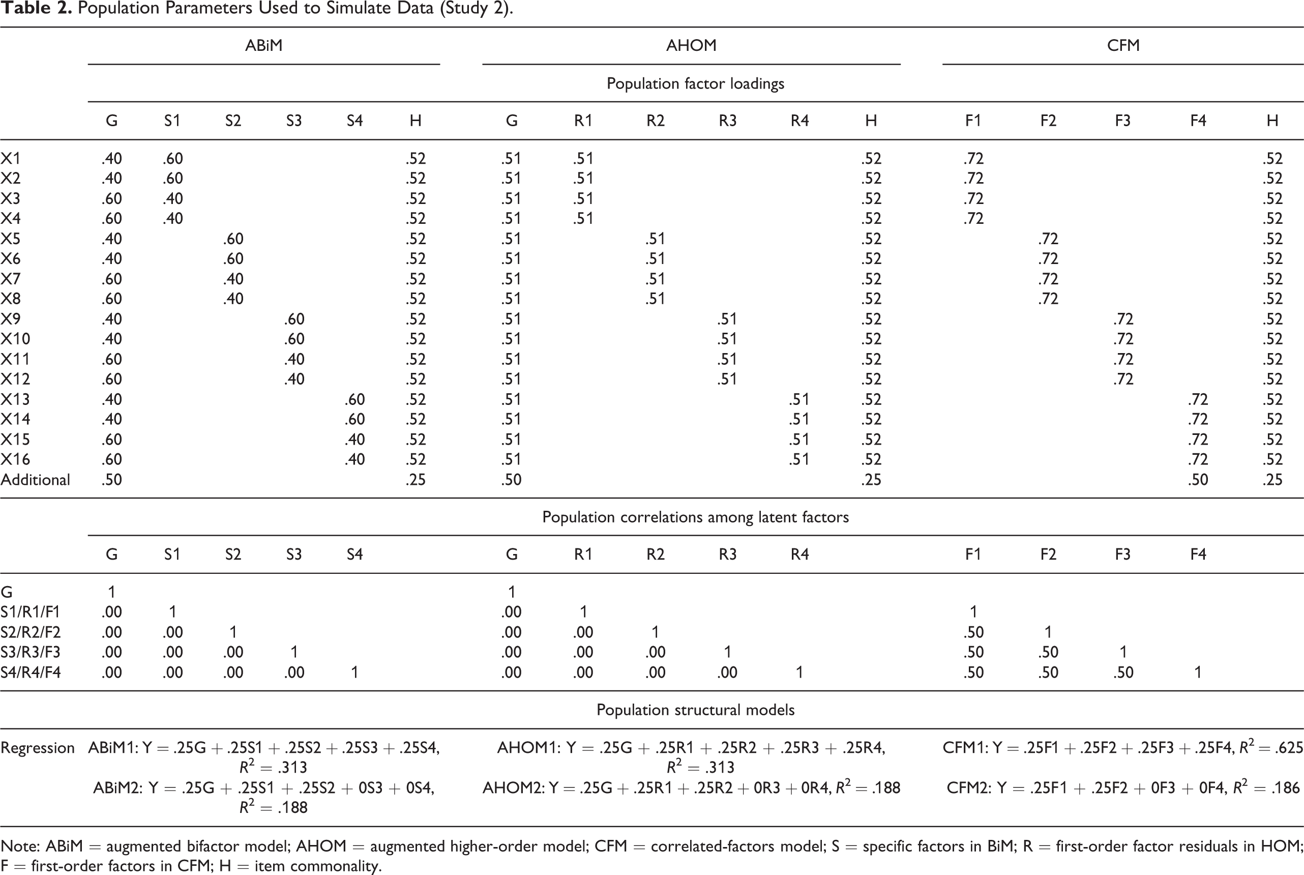
Note: ABiM = augmented bifactor model; AHOM = augmented higher-order model; CFM = correlated-factors model; S = specific factors in BiM; R = first-order factor residuals in HOM; F = first-order factors in CFM; H = item commonality.

In total, there were 84 conditions (3 × 2 × 2 × 7 = 84). Sample data were generated using the same procedure as Study 1. Maximum likelihood estimation was used. Replications that produced anomalous results were rejected until 1,000 valid replications were obtained. In addition, we also selected a sample size of 10,000 and ran 500 replications for each of these conditions to study the asymptotic performance of each model. All analyses were performed on valid replications.

When reporting results for ABiM1, AHOM1, and CFM1, we only focus on the general factor/higher-order factor and the first specific factor/facet because results for the other specific factor/facets were the almost identical to the first one. When reporting results for ABiM2, AHOM2, and CFM2, we focus on the general factor/higher-order factor, the first and the third specific factor/facet. That is because results for the second and the fourth specific factor/facet were almost identical to the first and the third, respectively. Also, we only report results for conditions whose number of indicators per facet was four because the overall pattern was very similar to conditions that had eight indicators per facet. Detailed results for the eight-item conditions can be found in the Supplemental Material (available in the online version of the journal).

Results

When the generation model was ABiM

As can be seen from Table 3, when the generation model was ABiM1 (βs = .25), fitting ABiM resulted in almost no bias in the regression coefficients and negligible bias in R ² once sample size reached 300. When sample size was 200, R ² was overestimated by 15%. Power for both the general factor and specific factors reached .85 when sample size reached 300. These findings are consistent with what we reported in Study 1. Fitting the AHOM led to somewhat different results. Although regression coefficients were still unbiased, the power to detect these effects decreased substantially compared to ABiM. Specifically, the power to detect the effect of the general factor and specific factor was only .42 and .30 when sample size was 200. Even when sample size reached 500, the power was still below 80%. Also, R ² was overestimated by 32% (bias = .100) when sample size was 200. Even though bias in R ² went down with increasing sample size and was asymptotically unbiased, it was overestimated by 11% (bias = .034) when sample size was 800. Fitting the CFM was more problematic. First, regression coefficient estimates of facets were underestimated by 44% (SOM = .138), and the power to detect the effect of these facets was far below .80 even for a sample size of 800. R ² was also constantly underestimated across sample sizes by 29% to approximately 36% (bias = .091∼.113).

Table 3.

Bias/Size of Misspecification and Power/Type I Error Rate When Data-Generating Model Was ABiM1 and ABiM2 (Study 2).

GM	Key Parameters	FM	Bias/Size of Misspecification								Power/Type I Error Rate
GM	Key Parameters	FM	200	300	400	500	600	700	800	10000	200	300	400	500	600	700	800	10000
ABiM1	R ² = .313	ABiM	.048	.029	.024	.016	.017	.013	.011	–.003	1.00	1.00	1.00	1.00	1.00	1.00	1.00	1.00
		AHOM	.101	.086	.063	.054	.050	.049	.035	.008	1.00	1.00	1.00	1.00	1.00	1.00	1.00	1.00
		CFM	–.092	–.101	–.108	–.110	–.112	–.114	–.113	–.123	1.00	1.00	1.00	1.00	1.00	1.00	1.00	1.00
	β _G = .25	ABiM	.002	.003	.000	.002	–.001	–.001	.002	.000	.75	.89	.95	.99	.99	1.00	1.00	1.00
		AHOM	.012	.002	.001	.002	–.002	–.003	.003	.000	.42	.54	.65	.73	.81	.84	.90	1.00
		CFM	—	—	—	—	—	—	—	—	—	—	—	—	—	—	—	—
	β_S1/R1/F1 = .25	ABiM	–.004	.001	–.001	–.003	–.001	–.002	–.001	.000	.70	.87	.92	.98	.99	1.00	1.00	1.00
		AHOM	–.012	.006	.000	.001	.002	.003	.001	.000	.30	.51	.58	.66	.75	.81	.87	1.00
		CFM	–.111	–.101	–.112	–.112	–.113	–.113	–.110	–.110	.23	.33	.39	.43	.50	.59	.65	1.00
ABiM2	R ² = .188	ABiM	.058	.036	.027	.022	.015	.014	.015	.003	1.00	1.00	1.00	1.00	1.00	1.00	1.00	1.00
		AHOM	.137	.093	.073	.056	.046	.042	.037	.003	1.00	1.00	1.00	1.00	1.00	1.00	1.00	1.00
		CFM	.021	.008	.004	.000	–.003	–.003	–.002	–.008	1.00	1.00	1.00	1.00	1.00	1.00	1.00	1.00
	β _G = .25	ABiM	.006	–.001	.000	.003	–.001	.001	–.001	.000	.76	.88	.95	.98	1.00	1.00	1.00	1.00
		AHOM	.005	.001	–.001	.004	–.001	–.001	–.002	.000	.42	.53	.65	.74	.83	.86	.91	1.00
		CFM	—	—	—	—	—	—	—	—	—	—	—	—	—	—	—	—
	β_S1/R1/F1 = .25	ABiM	–.005	–.002	–.001	–.003	–.005	–.002	.002	.000	.68	.82	.92	.96	.98	.99	1.00	1.00
		AHOM	–.001	.000	.003	–.002	–.002	.003	.007	.000	.33	.46	.60	.64	.73	.80	.86	1.00
		CFM	.045	.043	.043	.040	.039	.041	.046	.040	.67	.84	.91	.97	.99	1.00	1.00	1.00
	β_S3/R3/F3 = 0	ABiM	–.007	.003	–.002	.002	–.002	–.002	–.001	.000	.08	.07	.07	.05	.06	.05	.05	.05
		AHOM	–.007	.000	–.001	.001	–.001	.001	.001	.000	.04	.05	.06	.04	.05	.05	.04	.05
		CFM	–.087	–.075	–.081	–.074	–.078	–.080	–.080	–.080	.12	.11	.17	.15	.19	.24	.27	.99

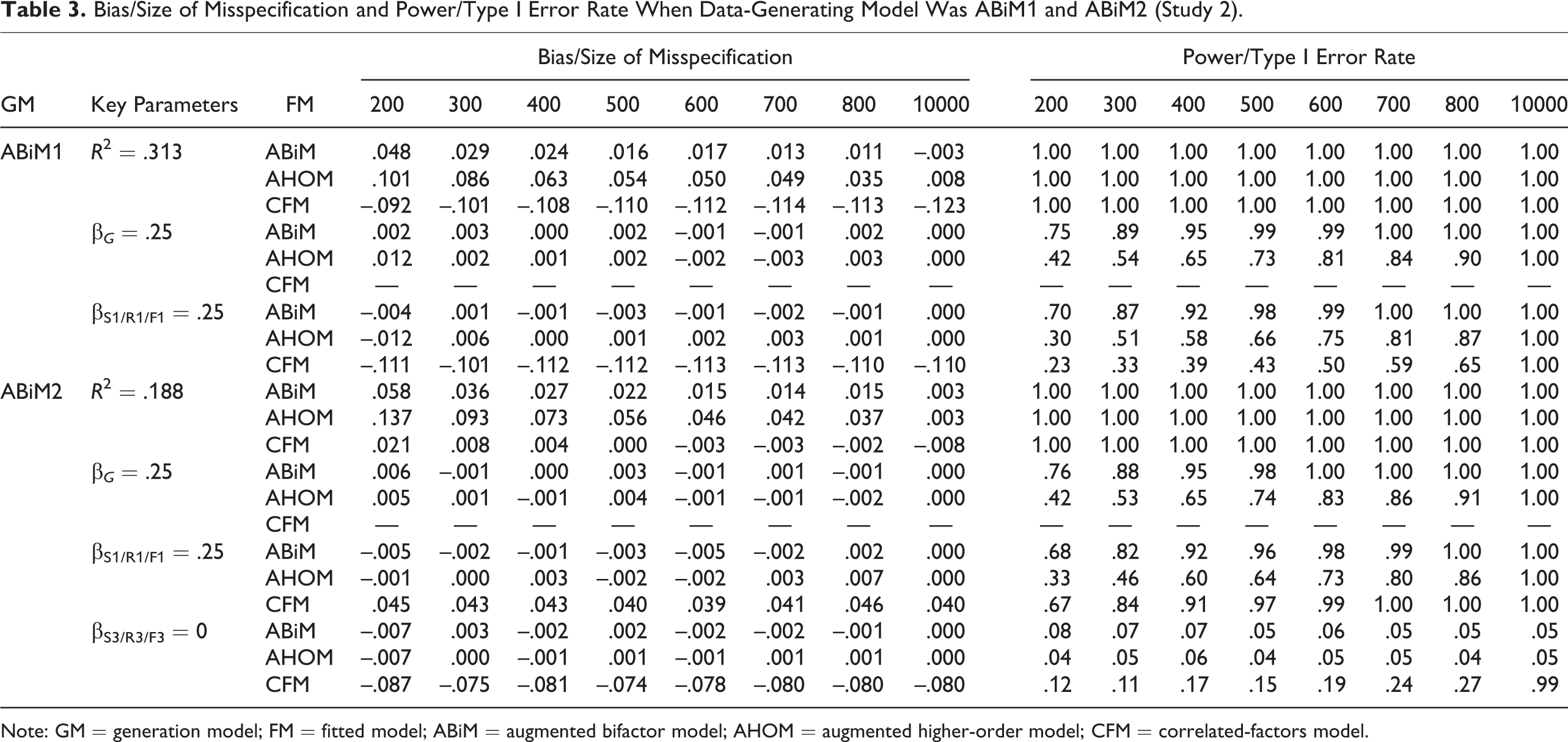
Note: GM = generation model; FM = fitted model; ABiM = augmented bifactor model; AHOM = augmented higher-order model; CFM = correlated-factors model.

When the ABiM2 was the generation model (β _G = β _S ₁ = .25, β _S ₃ = 0), fitting ABiM resulted in almost no bias in regression coefficients. The power to detect the effect of the general factor and the first specific factor exceeded .80 when sample size reached 300. Type I error rate associated with the third specific factor was close to .05 (.050∼.081) across sample sizes. However, R ² was overestimated by 31% (bias = .058) when sample size was 200. Overestimation of R ² only dropped below 10% when sample size reached 600. Fitting AHOM resulted in no bias in regression coefficients. However, the power to detect the effect of the general factor and the first specific factor was substantially lower, although the Type I error rate associated with the third specific factor was close to .05. Moreover, R ² was more overestimated with AHOM despite being asymptotically unbiased. Specifically, R ² was overestimated by 73% (bias = .139) at a sample size of 200 and by 30% (bias = .056) at a sample size of 500. Even when sample size reached 800, it was still overestimated by 20% (bias = .038). Fitting CFM yielded a different pattern of results. First, compared to the corresponding regression coefficients of specific factors in the population model, the regression coefficient of the first facet was overestimated by about 18% (SOM = .040∼.045), whereas those of the third facet were underestimated by about 33% relative to .25 (SOM = –.0875 to approximately –.075). Second, the power to detect the effect of the first facet was close to that in the bifactor model and higher than AHOM. But the Type I error rate associated with the third facet was .12 and increased with sample size. Surprisingly, the bias in R ² was negligible when sample size reached 300.

When the generation model was AHOM

As shown in Table 4, when the generation model was AHOM1 (βs = .25), fitting ABiM resulted in negligible bias in regression coefficients once sample size reached 300. However, the power to detect the effect of the general factor and specific factors did not reach .80 until sample size reached 600. R ² was also moderately overestimated by 12% to approximately 33% (bias = .038∼.119) until sample size was 800. Results for fitting AHOM were similar to ABiM: There was almost negligible bias in regression coefficients; the power was below .80 until sample size was 600; R ² was overestimated by 11% to approximately 26% (bias = .034∼.081) until sample size reached 800. Fitting CFM led to consistent underestimation of the regression coefficients of facets by 33% to approximately 44% (SOM = .083∼.110), which caused low power (the power was only .70 even at a sample size of 800). R ² was also consistently underestimated by 27% to approximately 35% (bias = .068∼.088).

Table 4.

Bias/Size of Misspecification and Power/Type I Error Rate When Data-Generating Model Was AHOM1 and AHOM2 (Study 2).

GM	Key Parameters	FM	Bias/Size of Misspecification								Power/Type I Error Rate
GM	Key Parameters	FM	200	300	400	500	600	700	800	1,0000	200	300	400	500	600	700	800	1,0000
AHOM1	R ² = .313	ABiM	.104	.068	.062	.059	.052	.036	.028	.008	1.00	1.00	1.00	1.00	1.00	1.00	1.00	1.00
		AHOM	.081	.053	.044	.050	.044	.034	.028	.008	1.00	1.00	1.00	1.00	1.00	1.00	1.00	1.00
		CFM	–.084	–.094	–.102	–.105	–.106	–.108	–.109	–.113	1.00	1.00	1.00	1.00	1.00	1.00	1.00	1.00
	β _G = .25	ABiM	.042	.024	.009	–.002	–.003	.000	.002	.000	.62	.67	.71	.76	.82	.88	.92	1.00
		AHOM	.023	.018	.007	–.002	–.003	–.001	.000	.000	.48	.60	.68	.74	.79	.87	.92	1.00
		CFM	—	—	—	—	—	—	—	—	—	—	—	—	—	—	—	—
	β_S1/R1/F1 = .25	ABiM	–.042	–.021	–.012	.001	.003	.000	–.004	.000	.43	.56	.67	.76	.83	.87	.89	1.00
		AHOM	–.021	–.015	–.008	.001	.003	.002	–.001	.000	.31	.47	.61	.70	.80	.85	.89	1.00
		CFM	–.108	–.105	–.108	–.110	–.107	–.106	–.109	–.110	.25	.36	.42	.52	.59	.67	.70	1.00
AHOM2	R ² = .188	ABiM	.166	.107	.080	.060	.046	.041	.031	.003	1.00	1.00	1.00	1.00	1.00	1.00	1.00	1.00
		AHOM	.111	.083	.061	.046	.037	.036	.026	.003	1.00	1.00	1.00	1.00	1.00	1.00	1.00	1.00
		CFM	.014	.007	.003	–.003	–.004	–.005	–.007	–.008	1.00	1.00	1.00	1.00	1.00	1.00	1.00	1.00
	β _G = .25	ABiM	.015	.002	.004	.004	.001	–.002	.001	.000	.58	.62	.72	.77	.82	.87	.90	1.00
		AHOM	.006	–.001	.004	.003	–.001	–.003	–.001	.000	.43	.53	.69	.75	.80	.84	.90	1.00
		CFM	—	—	—	—	—	—	—	—	—	—	—	—	—	—	—	—
	β_S1/R1/F1 = .25	ABiM	–.022	–.004	–.005	–.005	–.005	.000	–.004	.000	.48	.61	.67	.72	.79	.85	.88	1.00
		AHOM	–.010	–.001	–.004	–.003	–.004	.002	–.002	.000	.34	.52	.59	.70	.77	.84	.87	1.00
		CFM	.033	.037	.039	.037	.034	.036	.035	.030	.69	.86	.94	.98	.99	1.00	1.00	1.00
	β_S3/R3/F3 = 0	ABiM	–.018	–.004	–.010	–.004	–.004	.001	–.004	.000	.16	.13	.12	.11	.11	.09	.07	.05
		AHOM	–.007	–.001	–.010	–.002	–.003	.002	–.003	.000	.03	.04	.05	.04	.05	.05	.04	.04
		CFM	–.070	–.068	–.075	–.066	–.069	–.068	–.070	–.070	.10	.10	.15	.14	.20	.20	.23	.99

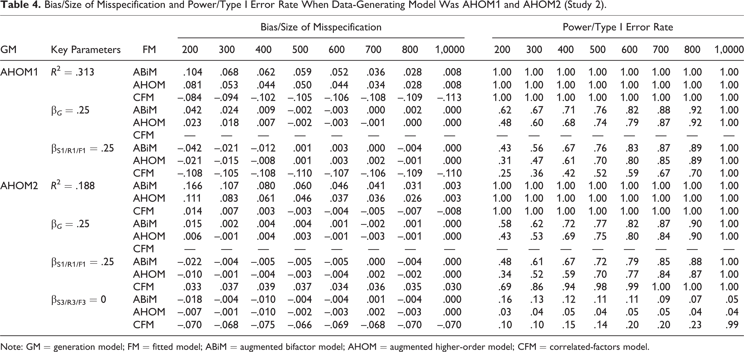
Note: GM = generation model; FM = fitted model; ABiM = augmented bifactor model; AHOM = augmented higher-order model; CFM = correlated-factors model.

When the generation model was AHOM2 (β _G = β _R ₁ = .25, β _R ₃ = 0) and the fitted model was ABiM, there was little bias in regression coefficients when sample size reached 300. But the power to detect the effect of the general factor and the first specific factor did not reach .80 until sample size was 600, which was lower than when the generation model was ABiM2. The Type I error rate for the third specific factor was .16 when sample size was 200. It decreased to .07 when sample size reached 800. R ² was overestimated by 16% to approximately 88% (bias = .031∼.165), especially when sample size was small. The pattern for fitting AHOM was close to ABiM, except that AHOM led to somewhat lower power, better Type I error rate, and slightly lower overestimation of R ². Fitting CFM resulted in different results. First, the regression coefficient of the first factor was consistently overestimated by about 12% (SOM = .030), and the regression coefficient of the third factor was consistently underestimated by about 28% (SOM = .070). Correspondingly, the power to detect the effect of the first factor reached .80 at a sample size of 300. The Type I error rate for the third facet was .10 at a sample size of 200 and increased with sample size. As found in conditions where the generation model was ABiM2, there was negligible bias in R ² for CFM.

When the generation model was CFM

As shown in Table 5, when the generation model was CFM1 (βs = .25), fitting both ABiM and AHOM led to consistent underestimation of the regression coefficients by about 25% (SOM = –.06). Consequently, the power to detect the effect of the first facet did not reach .80 until sample size was 800. Surprisingly, bias in R ² was negligible once sample reached 400 for ABiM and 300 for AHOM. Fitting CFM resulted in no bias in regression coefficients and R ² across sample sizes. The power to detect the effect of the first facet was close to .80 even at a sample size of 200.

Table 5.

Bias/Size of Misspecification and Power/Type I Error Rate When Data-Generating Model Was CFM1 and CFM2 (Study 2).

GM	Key Parameters	FM	Bias/Size of Misspecification								Power/Type I Error Rate
GM	Key Parameters	FM	200	300	400	500	600	700	800	1,0000	200	300	400	500	600	700	800	1,0000
CFM1	R ² = .625	ABiM	.094	.077	.060	.045	.039	.031	.029	–.005	1.00	1.00	1.00	1.00	1.00	1.00	1.00	1.00
		AHOM	.076	.054	.044	.033	.030	.025	.023	–.005	1.00	1.00	1.00	1.00	1.00	1.00	1.00	1.00
		CFM	.014	.011	.010	.004	.006	.004	.004	–.005	1.00	1.00	1.00	1.00	1.00	1.00	1.00	1.00
	β_S1/R1/F1 = .25	ABiM	–.053	–.068	–.063	–.060	–.060	–.063	–.066	–.060	.55	.57	.66	.71	.77	.80	.82	1.00
		AHOM	–.057	–.063	–.062	–.061	–.061	–.062	–.063	–.060	.36	.47	.58	.66	.73	.77	.81	1.00
		CFM	.003	–.001	.000	–.001	.001	–.001	.000	.000	.79	.91	.97	1.00	1.00	1.00	1.00	1.00
CFM2	R ² = .186	ABiM	.188	.145	.100	.080	.060	.051	.048	.002	1.00	1.00	1.00	1.00	1.00	1.00	1.00	1.00
		AHOM	.136	.101	.072	.056	.047	.038	.037	.002	1.00	1.00	1.00	1.00	1.00	1.00	1.00	1.00
		CFM	.028	.018	.014	.009	.010	.006	.006	.002	1.00	1.00	1.00	1.00	1.00	1.00	1.00	1.00
	β_S1/R1/F1 = .25	ABiM	–.054	–.045	–.045	–.042	–.049	–.050	–.044	–.050	.43	.53	.58	.63	.68	.71	.77	1.00
		AHOM	–.046	–.041	–.047	–.045	–.049	–.050	–.045	–.050	.28	.40	.47	.54	.61	.67	.74	1.00
		CFM	.001	.003	.002	.000	.000	–.005	.002	.000	.60	.79	.88	.92	.96	.99	1.00	1.00
	β_S3/R3/F3 = 0	ABiM	.013	.022	.026	.028	.019	.027	.025	.020	.16	.17	.14	.12	.11	.11	.13	.19
		AHOM	.020	.025	.025	.026	.020	.027	.024	.020	.03	.04	.04	.06	.05	.05	.05	.18
		CFM	–.005	–.005	.000	.000	–.003	.004	.000	.000	.06	.06	.05	.06	.05	.07	.05	.04

Note: GM = generation model; FM = fitted model; ABiM = augmented bifactor model; AHOM = augmented higher-order model; CFM = correlated-factors model.

When the generation model was CFM2 (β _F ₁ = .25, β _F ₃ = 0), fitting both ABiM and AHOM led to consistent underestimation of the regression coefficient of the first facet by about 18% (SOM = –.045) and overestimation of the regression coefficient of the third facet by about 10% relative to .25. The power to detect the effect of the first facet did not reach .80 even at a sample size of 800. The Type I error rate associated with the third facet of the ABiM ranged from about .10 to approximately .16, whereas that of the AHOM stayed closer to the nominal level across sample sizes. Regarding R ², even though it was asymptotically unbiased, it was severely overestimated for both ABiM and AHOM, especially when sample size was small. For example, at a sample size of 200, R ² of ABiM and AHOM was overestimated by 101% and 73% (bias = .188 and .136), respectively. Even when sample size reached 800, R ² was overestimated by 26% and 20% (bias = .048 and .037) for ABiM and AHOM. Fitting CFM resulted in virtually no bias in regression coefficients and R ² across sample sizes. The power to detect the effect of the first facet was close to .80 even at a sample size of 300. The Type I error rate associated with the third facet remained around .05 across sample sizes.

Discussion

The results shown in Table 3, 4, and 5 demonstrated the importance of analyzing one’s data with an appropriate model: Fitting a misspecified model sometimes led to very misleading results. A critical decision for researchers is whether to adopt a hierarchical representation (ABiM and AHOM) or a correlated factor representation (CFM). This had a great influence on key results. For example, when the data-generation model was ABiM1 or AHOM1, fitting CFM severely underestimated the regression coefficients of specific factors, thus causing the power to be below .80 even at a sample size of 800. R ² was also consistently underestimated. This means that researchers would be likely to falsely conclude that facets do not have incremental validity and the overall predictive validity of the construct is small. On the other hand, when only some of the specific factors have incremental validity (ABiM2 and AHOM2), fitting CFM is likely to overestimate the regression coefficients of facets that have nonzero incremental validity. Specific factors with zero incremental validity were also found to be predictive but in the negative direction. R ², however, was almost unbiased once sample size reached 300. When CFM1 was the data-generation model, fitting either ABiM or AHOM moderately underestimated the regression coefficients of facets and thus had lower power. But R ² was accurately recovered once sample size reached 300. When CFM2 was the data-generation model and ABiM or AHOM was fitted, the regression coefficients of facets that had nonzero incremental validity were slightly underestimated, and the regression coefficients of facets with zero incremental validity were slightly overestimated. But statistical power was reasonable in sufficiently large samples despite slightly high Type I error rates for ABiM. It is interesting to note that ABiM and AHOM had very similar asymptotic performances in terms of bias, power, and Type I error rate regardless of data-generation models. Both ABiM and AHOM accurately recovered R ² regardless of data-generation models. For a sample of several hundred, ABiM performed somewhat better than AHOM in terms of power and similarly in terms of regression coefficient bias. But it had slightly higher Type I error rates and larger relative bias of R ² for small to modest sample sizes (e.g., n < 600).

Even though ABiM and AHOM accurately recovered R ² regardless of data-generation models asymptotically, typical sample sizes often seen in organizational studies do not seem to suffice to achieve this desirable performance. This result occurred because the precision (standard deviation) of estimated regression coefficients in ABiM and AHOM were about 1 times larger than those in CFM in many cases (AHOMs had even lower precision than ABiMs), indicating that regression coefficients in ABiM and AHOM vary across replications more than CFM. When they were squared to obtain R ², upward estimation errors were more influential than downward errors, thus leading to overestimation of R ². This problem is particularly severe in cases where the true regression coefficients of some specific factors were zero. Any deviation from zero will result in overestimation of R ² because the squared estimate is always greater than zero.

General Discussion

Despite their increasing popularity, there is still ambiguity about whether and how bifactor models should be used to examine the predictive validity of constructs. Specifically, little attention has been paid to the nonidentification problems of bifactor models when used in predictive models. Moreover, little work has investigated the practical consequences of adopting different conceptualizations of constructs when examining predictive validity. The present study first reviewed the statistical problems of bifactor models and existing solutions. We then adopted the augmented bifactor model as a strategy for addressing these problems. A Monte Carlo simulation study showed that this strategy effectively reduced the likelihood of anomalous results, increased power, and maintained Type I error rates close to the nominal level. The second simulation study demonstrated the practical consequences of adopting different models for constructs maybe substantial: Researchers may arrive at different conclusions regarding the predictive validity of hierarchical constructs depending on their choice of models. This is certainly problematic.

In general, ABiM led to correct substantive conclusions regarding incremental validity of facets regardless of the true data-generation model given a sufficiently large sample (n ≥ 600), but R ² values are likely to be substantially overestimated. In the following, we discuss pros and cons of using bifactor models for prediction in light of our current findings, highlight several implications, and provide practical recommendations for planning future research.

Bifactor models and the augmentation strategy

As typically implemented, BiM specifies general and specific factors as orthogonal components, thus allowing researchers to examine their psychometric properties independently and additively. These features are particularly relevant for studying the predictive validity of hierarchical domains; because all factors are orthogonal, regression coefficients can be directly interpreted as the independent contribution of each component. However, our first series of simulations showed that BiM is prone to problems (nonconvergence, etc.) and inadequate power when the number of indicators per facet is modest (e.g., four) and sample size is small to moderate (n < 600). Nonetheless, many constructs in organizational research are measured by a small number of indicators (Hinkin, 1995). Typical sample sizes used in organizational research are also often in the range we examined (Su et al., 2019). Furthermore, interpretation of factors in BiM is problematic in many cases (Eid et al., 2017). These concerns limit the potential usefulness of BiMs.

ABiM inherits the conceptual advantage of BiM but seems to mitigate the problem of nonidentification and construct ambiguity. The additional indicator largely eliminates anomalous results and thus improves the statistical performance of BiMs. ABiMs work reasonably well even in the settings where BiM fails. In addition, unlike BiM, whose factors have ambiguous construct validity, the augmenting indicator gives clear construct meanings to factors in ABiM. The general factor is defined as the augmenting indicator, and its construct meaning should not change as facets are added or removed. Similarly, specific factors are residualized facets relative to the augmenting indicator. Interested readers are encouraged to refer to Eid et al. (2017) for an excellent discussion. An additional advantage of ABiM is that it encourages researchers to think deeper about the construct’s meaning because an indicator of the general factor is needed. This requirement may, in fact, facilitate theory development. Moreover, ABiM seems more robust to some model misspecifications. Although AHOM has the same conceptual virtues and performs almost identically to ABiM asymptotically, its statistical performance at more modest sample levels is less optimal. CFM seems more limited. First, unambiguous interpretation of regression coefficients is not possible when the facets are moderately to highly correlated. Second, it may result in underestimation of the overall predictive validity of hierarchical constructs and lead to wrong conclusions. In sum, the augmentation strategy seems to solve the statistical and conceptual problems arising with BiM while maintaining its intuitive appeal. CFM is not recommended for studying hierarchical constructs from both a conceptual and pragmatic perspective. Whether a construct is hierarchical or not, however, is a topic that has been debated since the time of Spearman and Thurstone.

Considerations of adopting ABiMs and recommendations

Despite the advantages discussed previously, researchers should still be cautious when adopting ABiM because it still inherits some problems of BiM. First, BiMs have an overfitting tendency. In reality, researchers do not know the true model underlying the data but still need to choose one to answer research questions. The common practice is to fit different models to the data and use various model fit indices to select the best-fitting model. BiMs in past studies have often stood out as best fitting (Rodriguez, Reise, & Haviland, 2016). However, recent studies suggested that BiMs tend to beat other models (e.g., HOM and CFM) because they have an overfitting tendency. For example, BiMs can absorb cross-loadings, correlated residuals, and population heterogeneity through the general factor (Murray & Johnson, 2013; Raykov et al., 2019) and fit invalid or even random data (Bonifay & Cai, 2017; Reise et al., 2016). Therefore, researchers are recommended to not only examine model comparison results based on multiple fit indices (e.g., comparative fit index, Tucker-Lewis index, root mean square error of approximation, standardized root mean square residual, Akaike information criterion, Bayesian information criterion) but also to conduct additional robustness check before making their final decision. For example, researchers can use the iteratively reweighted least squares estimation method to ensure that ABiM fits better because it better describes the response process instead of just tolerating invalid responses (Reise et al., 2016). Moreover, researchers are strongly encouraged to evaluate ABiM solutions through statistics such as various omega reliability coefficients and factor determinacy. If these statistics are too low, the estimated ABiM solution may not be meaningful despite good fit statistics. Another less well-known but extremely useful statistic for robustness check is the construct reliability—or more recently termed as construct replicability—that quantifies “how well a latent variable is represented by a given set of observed indicators, and, thus, replicable across studies” (Rodriguez et al., 2016, p.143; Hancock & Mueller, 2001). A meaningful ABiM solution should have moderate to high construct replicability for both the general factor and specific factors. Researchers can refer to Rodriguez et al. (2016) for an excellent tutorial on the calculation and interpretation of these indices. In addition, replication using multiple samples is also encouraged.

Even when robustness checks and theories support the use of ABiMs, researchers should still be careful. Our first series of simulation showed that arbitrarily fixing some paths to zero can lead to overestimation in some cases. Therefore, it appears that all factors should be included in the prediction of external variables because this can keep estimation bias to a minimum and maintain power at an adequate level, even though the researcher is only interested in the general factor.

Our second study demonstrated that an R ² derived from ABiM is likely to be overestimated when sample size is small to moderate. A potential solution is to recalculate R ² by summing up the squares of only statistically significant standardized regression coefficients. Shrinkage formula may also be useful here. We sometimes noticed suspiciously large standard errors appear for regression coefficients (but not for other parameters) even though model estimation terminated normally. The appearance of very large standard errors is a sign of empirical underidentification (Rindskopf, 1984). Results obtained from such conditions are not trustworthy. Although there is no established guideline about how large is “suspiciously large,” researchers can compare standard errors of regression coefficients to the standard errors of other parameters. If the former is 3 or 4 times larger than the latter, there is cause for concern.

Sample size is another extremely important consideration for adopting ABiM. We recommend sample sizes of 500 or more in general. Such large sample sizes may be needed to keep the anomaly rate, power, Type I error rate, and estimation bias within acceptable ranges. This recommendation also coincides with Kretzschmar and Gignac’s (2019) finding that a sample size of 490 is required to achieve stable estimation of latent variable correlations in typical scenarios (ρ = .20, reliability = .70). Tailored simulations can be used to obtain a more precise estimate of sample size requirements because they vary substantially across contexts (Wolf et al., 2013). We provided R code on the Open Science Framework website that interested readers can use to assess their needs. Generally, we recommend against the use of ABiM if sample size is around or below 200.

How to find a good augmenting indicator is another important issue for researchers. We tentatively suggest two approaches. First, researchers can start from existing measures. Because most measures of hierarchical constructs were not developed using bifactor models, it is possible that some of these items may in fact only tap the general factor but are incorrectly assigned to a specific facet. Therefore, researchers can fit bifactor models to such measures. If some items consistently show high loadings on the general factor and trivial loadings on specific factors across multiple samples, such items may be considered as good candidates. Subsequently, researchers can ask a group of subject matter experts to make informed judgments about these candidate augmenting items. Items that survive statistical examinations and expert judgments can be used as augmenting items. Second, researchers can also write augmenting items from scratch. In some cases, the names of hierarchical constructs can be good candidates. For example, the item “I am an agreeable person” might be a good augmenting item for Agreeableness. In some other cases, items that do not refer to a specific target or domain also work (Eid et al., 2017). For example, Brunner and colleagues (2010) used items like “I’m good at most school subjects” to measure general academic self-concept. Fraley et al. (2015) also used items like “I find it easy to depend on people in close relationships” to measure global attachment styles. These items also need to go through statistical scrutiny before being used.

Last but not least, even though specific factors are constrained be orthogonal in the ABiM, it is not necessarily required for model identification. One of the anonymous reviewers recommended that researchers should always examine whether the orthogonal constraint is reasonable by comparing the fit of the ABiM and the more general bifactor-(S·I-1) model via a likelihood ratio test. If there is no statistically significant difference, then researchers can proceed with ABiM. If the ABiM fits significantly worse, researchers should adopt the more general bifactor-(S·I-1) model.

Considerations of choosing between models

A reviewer raised two interesting questions regarding model selection and model misfit that are not only pertinent to the current study but also may be important in broader contexts. While an elaborated discussion is beyond the scope of the current study, we decided to briefly address these questions in hope of raising awareness among researchers.

First, the reviewer asked, “What if a researcher’s specific data set is (1) supported by multiple models, (2) not supported by multiple models, (3) or there is mixed support?” (1) Although not widely recognized, some seemingly very different SEM models can indeed be equivalent in that they yield identical implied covariance or correlation matrices. Therefore, researchers are recommended to use the nesting and equivalence testing (NET) procedures to test for equivalence (Bentler & Satorra, 2010). If the NET procedure indicates equivalence, it is impossible to identify which model is the “true model” statistically. In such cases, researchers are encouraged to refer to their theories to decide which model is most appropriate. (2) If the data are not supported by multiple models, then the researcher might search for a better fitting model by looking for one that is very different from the one the researcher is using. Or one might just choose the model that fits the data the best. However, picking a model based on fit statistics, especially if they are not nested, can be very difficult: Some fit statistics may prefer one model, whereas other fit statistics may prefer another model (but see a recent description of the Vuong test for statistically comparing nonnested models by Merkle, You, & Preacher, 2016). (3) For mixed support, researchers should collect more or better data to help inform their decision. Researchers are encouraged to consider substantive theory while taking into consideration model parsimony.

The reviewer also asked when there is model misfit, how can a researcher probe the source of misfit (misfit from the measurement model or the structural model)? It is possible that the measurement model fits well but the structural model fits badly, or vice versa. However, traditional model fit evaluation focuses on global fit and does not differentiate misfit due to the measurement part and the structural part, which makes it hard to probe the source of misfit (if there is any). Psychometricians have considered these problems and proposed several solutions. For example, Anderson and Gerbing (1988) advocated a two-step strategy. A measurement model is first fitted to the data. If the measurement model shows acceptable fit, then researchers fit the full SEM model. A sequential chi-square test is then used to test specific hypotheses concerning the structural proportion of the model. There are also some fit indices for evaluating the fit of the structural model, including the target coefficients (TC2; Marsh, 1987), RMSEA-P (McDonald & Ho, 2002), and noncentrality structural covariance index, with a focus on the path model component of a composite model (NSCI-P; Williams & O'Boyle, 2011). Lance et al. (2016) provided a good summary of existing indices and developed six new indices. Recently, Thoemmes, Rosseel, and Textor (2018) also suggested the use of graphical criteria like d-separation and trek-separation for evaluating local fit. Modification indices and expected parameter change statistic can also aid with identifying model misfit. In sum, these methods can be used to evaluate fit of different components of an SEM model. Interested readers are encouraged to refer to these articles for more details.

Limitations and future directions

As with any simulation, the current studies are far from comprehensive. For example, all effect sizes were set to be .25, which is frequently seen and important, but other values should be investigated. We also did not consider conditions where the number of items per facet was unequal. Results may differ in these conditions. Another limitation is that we assumed a perfect structure with no cross-loadings and residual correlations. However, empirical data are likely to be messy with small cross-loadings (Asparouhov & Muthén, 2009). It is worth exploring how robust our conclusions are when nonzero cross-loadings are forced to zero rather than correctly modeled. Third, even though the augmentation strategy and increased sample size can reduce anomalous results, it is not always possible to add such an indicator (e.g., archival data analysis) or obtain more respondents (e.g., clinical population). In such cases, it might be interesting to examine whether Bayesian estimation can produce more accurate and stable parameter estimates by supplying informative priors. Fourth, we assumed orthogonality among BiM factors throughout this article because it allows straightforward explanations of regression coefficients of these factors. However, this is not required for the bifactor-(S·I -1) model (Eid et al., 2017). Future studies should examine the generalizability of our current findings in these conditions. Fifth, strictly speaking, adding new items to an existing scale is scale adaptation that might be problematic (Heggestad et al., 2019). Researchers should provide sufficient evidence to support validity of the adapted scale, particularly the construct validity of the augmenting item. Sixth, when comparing ABiM/AHOM and CFM, we compared regression coefficient estimates to the generating model parameters because researchers often interpret them similarly—as the unique contribution of a specific facet/factor. However, such comparisons are not fully statistically justified because predictors in these models may be scaled on somewhat different metrics. As suggested by one of the reviewers, a more justified comparison should be made between the expected regression coefficient for, say, CFM calculated based on the generating BiM model and estimated CFM regression coefficients. However, we are currently not aware of an established way to derive the expected value for CFM regression coefficients based on ABiM/AHOM generating models. In sum, small differences in estimation accuracy across misspecified and correctly specified models should not be overemphasized.

Conclusion

We reviewed the problems of BiMs in the context of studying the predictive validity of hierarchical constructs and proposed the augmentation strategy to address these problems. Simulation studies showed that BiMs are prone to anomalous results and low power, whereas ABiMs yield improved performance. We also investigated the practical consequences of adopting different conceptualizations of constructs and found that ABiMs have adequate power to arrive at correct conclusions regarding the incremental validity of facets and can reasonably recover the overall predictive validity regardless of the data-generation model given a sufficiently large sample size.

Supplemental Material

Supplemental Material, ORM_18_0126_R5_Supplementary_material_Tables - Using Bifactor Models to Examine the Predictive Validity of Hierarchical Constructs: Pros, Cons, and Solutions

Supplemental Material, ORM_18_0126_R5_Supplementary_material_Tables for Using Bifactor Models to Examine the Predictive Validity of Hierarchical Constructs: Pros, Cons, and Solutions by Bo Zhang, Tianjun Sun, Mengyang Cao and Fritz Drasgow in Organizational Research Methods

Footnotes

Appendix A

Appendix B

Appendix C

Appendix D

Appendix E

Appendix F

Authors’ Note

An earlier version of this article was presented on April 20, 2018, at the 33rd Annual Conference of the Society for Industrial and Organizational Psychology.

Acknowledgments

We would like to thank our Action Editor, Dr. Jonas Lang, and three anonymous reviewers for their extremely constructive feedback.

Declaration of Conflicting Interests

The author(s) declared no potential conflicts of interest with respect to the research, authorship, and/or publication of this article.

Funding

The author(s) received no financial support for the research, authorship, and/or publication of this article.

ORCID iD

Bo Zhang

Tianjun Sun

Supplemental Material

Supplemental material for this article is available online.

Notes

References

Aichholzer

Danner

Rammstedt

(2018). Facets of personality and “ideological asymmetries.” Journal of Research in Personality, 77, 90–100.

Anderson

J. C.

Gerbing

D. W.

(1984). The effect of sampling error on convergence, improper solutions, and goodness-of-fit indices for maximum likelihood confirmatory factor analysis. Psychometrika, 49(2), 155–173.

Ashton

M. C.

Lee

(2007). Empirical, theoretical, and practical advantages of the HEXACO model of personality structure. Personality and Social Psychology Review, 11(2), 150–166.

Asparouhov

Muthén

(2009). Exploratory structural equation modeling. Structural Equation Modeling: A Multidisciplinary Journal, 16(3), 397–438.

Asparouhov

Muthén

(2019). Nesting and equivalence testing for structural equation models. Structural Equation Modeling: A Multidisciplinary Journal, 26(2), 302–309.

Bentler

P. M.

Satorra

(2010). Testing model nesting and equivalence. Psychological Methods, 15(2), 111–123.

Bonifay

Cai

(2017). On the complexity of item response theory models. Multivariate Behavioral Research, 52(4), 465–484.

Boomsma

(1985). Nonconvergence, improper solutions, and starting values in LISREL maximum likelihood estimation. Psychometrika, 50(2), 229–242.

Bosco

F. A.

Aguinis

Singh

Field

J. G.

Pierce

C. A.

(2015). Correlational effect size benchmarks. Journal of Applied Psychology, 100(2), 431–449.

10.

Box

G. E.

(1976). Science and statistics. Journal of the American Statistical Association, 71(356), 791–799.

11.

Brunner

Keller

Dierendonck

Reichert

Ugen

Fischbach

Martin

(2010). The structure of academic self-concepts revisited: The nested Marsh/Shavelson model. Journal of Educational Psychology, 102(4), 964–981.

12.

Brunner

Nagy

Wilhelm

(2012). A tutorial on hierarchically structured constructs. Journal of Personality, 80(4), 796–846.

13.

Cai

(2010). A two-tier full-information item factor analysis model with applications. Psychometrika, 75(4), 581–612.

14.

Cai

Wirth

R. J

. (2013). flexMIRT®: A numerical engine for flexible multilevel multidimensional item analysis and test scoring (Version 2.00) [Computer software]. Vector Psychometric Group.

15.

Cai

Yang

J. S.

Hansen

(2011). Generalized full-information item bifactor analysis. Psychological Methods, 16(3), 221–248.

16.

Caspi

Houts

R. M.

Belsky

D. W.

Goldman-Mellor

S. J.

Harrington

Israel

Meier

M. H.

Ramrakha

Shalev

Poulton

Moffitt

T. E.

(2014). The p factor: one general psychopathology factor in the structure of psychiatric disorders? Clinical Psychological Science, 2(2), 119–137.

17.

Castro-Schilo

Grimm

K. J.

Widaman

K. F.

(2016). Augmenting the correlated trait–correlated method model for multitrait–multimethod data. Structural Equation Modeling: A Multidisciplinary Journal, 23(6), 798–818.

18.

Chalmers

R. P

. (2012). mirt: A multidimensional item response theory package for the R environment. Journal of Statistical Software, 48(6), 1–29.

19.

Chen

Bollen

K. A.

Paxton

Curran

P. J.

Kirby

J. B.

(2001). Improper solutions in structural equation models: Causes, consequences, and strategies. Sociological Methods & Research, 29(4), 468–508.

20.

Chen

F. F.

Hayes

Carver

C. S.

Laurenceau

J. P.

Zhang

(2012). Modeling general and specific variance in multifaceted constructs: A comparison of the bifactor model to other approaches. Journal of Personality, 80(1), 219–251.

21.

Chen

F. F.

Jing

Hayes

Lee

J. M.

(2013). Two concepts or two approaches? A bifactor analysis of psychological and subjective well-being. Journal of Happiness Studies, 14(3), 1033–1068.

22.

Chen

F. F.

West

S. G.

Sousa

K. H.

(2006). A comparison of bifactor and second-order models of quality of life. Multivariate Behavioral Research, 41(2), 189–225.

23.

Christensen

Mackinnon

A. J.

Korten

Jorm

A. F.

(2001). The “common cause hypothesis” of cognitive aging: Evidence for not only a common factor but also specific associations of age with vision and grip strength in a cross-sectional analysis. Psychology and Aging, 16(4), 588–599.

24.

Costa

P. T.

McCrae

R. R.

(1995). Domains and facets: Hierarchical personality assessment using the Revised NEO Personality Inventory. Journal of Personality Assessment, 64(1), 21–50.

25.

Debusscher

Hofmans

De Fruyt

(2017). The multiple face(t)s of state conscientiousness: Predicting task performance and organizational citizenship behavior. Journal of Research in Personality, 69, 78–85.

26.

Eid

Geiser

Koch

Heene

(2017). Anomalous results in G-factor models: Explanations and alternatives. Psychological Methods, 22(3), 541–562.

27.

Eid

Krumm

Koch

Schulze

(2018). Bifactor models for predicting criteria by general and specific factors: Problems of nonidentifiability and alternative solutions. Journal of Intelligence, 6(3), 1–23.

28.

Fraley

R. C.

Hudson

N. W.

Heffernan

M. E.

Segal

(2015). Are adult attachment styles categorical or dimensional? A taxometric analysis of general and relationship-specific attachment orientations. Journal of Personality and Social Psychology, 109(2), 354–368.

29.

Gibbons

R. D.

Bock

R. D.

Hedeker

Weiss

D. J.

Segawa

Bhaumik

D. K.

Kupfer

D. J.

Frank

Grochocinski

V. J.

Stover

(2007). Full-information item bifactor analysis of graded response data. Applied Psychological Measurement, 31(1), 4–19.

30.

Gibbons

R. D.

Hedeker

D. R.

(1992). Full-information item bi-factor analysis. Psychometrika, 57(3), 423–436.

31.

Gignac

G. E.

(2009). Partial confirmatory factor analysis: Described and illustrated on the NEO–PI–R. Journal of Personality Assessment, 91(1), 40–47.

32.

Gignac

G. E.

(2016). The higher-order model imposes a proportionality constraint: That is why the bifactor model tends to fit better. Intelligence, 55, 57–68.

33.

Grewal

Cote

J. A.

Baumgartner

(2004). Multicollinearity and measurement error in structural equation models: Implications for theory testing. Marketing Science, 23(4), 519–529.

34.

Gustafsson

J. E.

Balke

(1993). General and specific abilities as predictors of school achievement. Multivariate Behavioral Research, 28(4), 407–434.

35.

Hancock

G. R.

Mueller

R. O

. (2001). Rethinking construct reliability within latent variable systems. In Cudeck

du Toit

Sorbom

(Eds.), Structural equation modeling: Present and future (pp. 195–216). Scientific Software International.

36.

Heggestad

E. D.

Scheaf

D. J.

Banks

G. C.

Monroe Hausfeld

Tonidandel

Williams

E. B.

(2019). Scale adaptation in organizational science research: A review and best-practice recommendations. Journal of Management, 45(6), 2596–2627.

37.

Hinkin

T. R.

(1995). A review of scale development practices in the study of organizations. Journal of Management, 21(5), 967–988.

38.

Holzinger

K. J.

Swineford

(1937). The bi-factor method. Psychometrika, 2(1), 41–54.

39.

Idaszak

J. R.

Bottom

W. P.

Drasgow

(1988). A test of the measurement equivalence of the revised Job Diagnostic Survey: Past problems and current solutions. Journal of Applied Psychology, 73(4), 647–656.

40.

Jennrich

R. I.

Bentler

P. M.

(2011). Exploratory bi-factor analysis. Psychometrika, 76(4), 537–549.

41.

Jennrich

R. I.

Bentler

P. M.

(2012). Exploratory bi-factor analysis: The oblique case. Psychometrika, 77(3), 442–454.

42.

Jensen

A. R

. (1998). The g factor and the design of education In Sternberg

R. J.

Williams

W. M.

(Eds.), Intelligence, instruction, and assessment: Theory into practice (pp. 111–131). Lawrence Erlbaum Associates Publishers.

43.

Jeon

Rijmen

Rabe-Hesketh

(2014). Flexible item response theory modeling with FLIRT. Applied Psychological Measurement, 38(5), 404–405.

44.

Judge

T. A.

Rodell

J. B.

Klinger

R. L.

Simon

L. S.

Crawford

E. R.

(2013). Hierarchical representations of the five-factor model of personality in predicting job performance: Integrating three organizing frameworks with two theoretical perspectives. Journal of Applied Psychology, 98(6), 875–925.

45.

Kell

Lang

(2017). Specific abilities in the workplace: More important than g? Journal of Intelligence, 5(2), 13–31.

46.

Kell

Lang

(2018). The great debate: General ability and specific abilities in the prediction of important outcomes? Journal of Intelligence, 6(3), 1–23.

47.

Kretzschmar

Gignac

G. E.

(2019). At what sample size do latent variable correlations stabilize? Journal of Research in Personality, 80, 17–22.

48.

Lance

C. E.

Beck

S. S.

Fan

Carter

N. T.

(2016). A taxonomy of path-related goodness-of-fit indices and recommended criterion values. Psychological Methods, 21(3), 388–404.

49.

Mansolf

Reise

S. P.

(2016). Exploratory bifactor analysis: The Schmid-Leiman orthogonalization and Jennrich-Bentler analytic rotations. Multivariate Behavioral Research, 51(5), 698–717.

50.

Markon

K. E.

(2019). Bifactor and hierarchical models: Specification, inference, and interpretation. Annual Review of Clinical Psychology, 15, 51–69.

51.

Marsh

H. W.

(1987). The hierarchical structure of self-concept and the application of hierarchical confirmatory factor analysis. Journal of Educational Measurement, 24(1), 17–39.

52.

Maslach

Jackson

S. E.

Leiter

M. P

. (1996). Maslach Burnout Inventory manual (3rd ed.). Consulting Psychologists Press.

53.

Mason

C. H.

Perreault

W. D.

Jr , (1991). Collinearity, power, and interpretation of multiple regression analysis. Journal of Marketing Research, 28(3), 268–280.

54.

McAbee

S. T.

Oswald

F. L.

Connelly

B. S.

(2014). Bifactor models of personality and college student performance: A broad versus narrow view. European Journal of Personality, 28(6), 604–619.

55.

McDonald

R. P.

M. H. R.

(2002). Principles and practice in reporting structural equation analyses. Psychological Methods, 7(1), 64–82.

56.

McGrew

K. S.

(2009). CHC theory and the human cognitive abilities project: Standing on the shoulders of the giants of psychometric intelligence research. Intelligence, 37, 1–10.

57.

Merkle

E. C.

You

Preacher

K. J.

(2016). Testing nonnested structural equation models. Psychological Methods, 21(2), 151–163.

58.

Mike

King

Oltmanns

T. F.

Jackson

J. J.

(2018). Obsessive, compulsive, and conscientious? The relationship between OCPD and personality traits. Journal of Personality, 86(6), 952–972.

59.

Moshagen

Hilbig

B. E.

Zettler

(2018). The dark core of personality. Psychological Review, 125(5), 656–688.

60.

Murray

A. L.

Johnson

(2013). The limitations of model fit in comparing the bi-factor versus higher-order models of human cognitive ability structure. Intelligence, 41(5), 407–422.

61.

Muthén

L. K.

Muthén

B. O.

(2002). How to use a Monte Carlo study to decide on sample size and determine power. Structural Equation Modeling: A Multidisplinary Journal, 9(4), 599–620.

62.

Cao

Marsh

H. W.

Tay

Seligman

M. E.

(2017). The factor structure of the Values in Action Inventory of Strengths (VIA-IS): An item-level exploratory structural equation modeling (ESEM) bifactor analysis. Psychological Assessment, 29(8), 1053–1058.

63.

Nye

C. D.

Chernyshenko

O. S.

Stark

Drasgow

Phillips

H. L.

Phillips

J. B.

Campbell

J. S.

(2020). More than g: Evidence for the incremental validity of performance-based assessments for predicting training performance. Applied Psychology: An International Review, 69(2), 302–324.

64.

Olea

M. M.

Ree

M. J.

(1994). Predicting pilot and navigator criteria: Not much more than g. Journal of Applied Psychology, 79(6), 845–851.

65.

Raykov

Marcoulides

G. A.

Menold

Harrison

(2019). Revisiting the bi-factor model: Can mixture modeling help assess its applicability? Structural Equation Modeling: A Multidisciplinary Journal, 26(1), 110–118.

66.

Ree

M. J.

Carretta

T. R.

Teachout

M. S.

(2015). Pervasiveness of dominant general factors in organizational measurement. Industrial and Organizational Psychology, 8(3), 409–427.

67.

Ree

M. J.

Earles

J. A.

(1991). Predicting training success: Not much more than g. Personnel Psychology, 44(2), 321–332.

68.

Ree

M. J.

Earles

J. A.

Teachout

M. S.

(1994). Predicting job performance: Not much more than g. Journal of Applied Psychology, 79(4), 518–524.

69.

Reise

S. P.

(2012). The rediscovery of bifactor measurement models. Multivariate Behavioral Research, 47(5), 667–696.

70.

Reise

S. P.

Kim

D. S.

Mansolf

Widaman

K. F.

(2016). Is the bifactor model a better model or is it just better at modeling implausible responses? Application of iteratively reweighted least squares to the Rosenberg Self-Esteem Scale. Multivariate Behavioral Research, 51(6), 818–838.

71.

Reise

S. P.

Moore

T. M.

Haviland

M. G.

(2010). Bifactor models and rotations: Exploring the extent to which multidimensional data yield univocal scale scores. Journal of Personality Assessment, 92(6), 544–559.

72.

Reise

S. P.

Morizot

Hays

R. D.

(2007). The role of the bifactor model in resolving dimensionality issues in health outcomes measures. Quality of Life Research, 16(1), 19–31.

73.

Reise

S. P.

Scheines

Widaman

K. F.

Haviland

M. G.

(2013). Multidimensionality and structural coefficient bias in structural equation modeling: A bifactor perspective. Educational and Psychological Measurement, 73(1), 5–26.

74.

Revelle

. (2018). psych: Procedures for personality and psychological research. https://CRAN.R-project.org/package=psychVersion=1.8.12.

75.

Richard

F. D.

Bond

C. F.

Jr Stokes-Zoota

J. J.

(2003). One hundred years of social psychology quantitatively described. Review of General Psychology, 7(4), 331–363.

76.

Rindskopf

(1984). Structural equation models: Empirical identification, Heywood cases, and related problems. Sociological Methods & Research, 13(1), 109–119.

77.

Roberts

B. W.

Chernyshenko

O. S.

Stark

Goldberg

L. R.

(2005). The structure of conscientiousness: An empirical investigation based on seven major personality questionnaires. Personnel Psychology, 58(1), 103–139.

78.

Rodriguez

Reise

S. P.

Haviland

M. G.

(2016). Evaluating bifactor models: Calculating and interpreting statistical indices. Psychological Methods, 21(2), 137–150.

79.

Rosseel

(2012). Lavaan: An R package for structural equation modeling and more. Version 0.5–12 (BETA). Journal of Statistical Software, 48(2), 1–36.

80.

Salthouse

T. A.

(1998). Relation of successive percentiles of reaction time distributions to cognitive variables and adult age. Intelligence, 26(2), 153–166.

81.

Samuel

D. B.

Widiger

T. A.

(2008). A meta-analytic review of the relationships between the five-factor model and DSM-IV-TR personality disorders: A facet level analysis. Clinical Psychology Review, 28(8), 1326–1342.

82.

Schaufeli

W. B.

Bakker

(2003). Utrecht work engagement scale (UWES) preliminary manual [Version 1, November 2003]. Utrecht University: Occupational Health Psychology Unit.

83.

Schmid

Leiman

J. M.

(1957). The development of hierarchical factor solutions. Psychometrika, 22(1), 53–61.

84.

Schmidt

F. L.

Hunter

(2004). General mental ability in the world of work: Occupational attainment and job performance. Journal of Personality and Social Psychology, 86(1), 162–173.

85.

Schmiedek

S. C.

(2004). Toward an alternative representation for disentangling age-associated differences in general and specific cognitive abilities. Psychology and Aging, 19(1), 40–56.

86.

Sigal

M. J.

Chalmers

R. P.

(2016). Play it again: Teaching statistics with Monte Carlo simulation. Journal of Statistics Education, 24(3), 136–156.

87.

Soto

C. J.

John

O. P.

(2017). The next Big Five Inventory (BFI-2): Developing and assessing a hierarchical model with 15 facets to enhance bandwidth, fidelity, and predictive power. Journal of Personality and Social Psychology, 113(1), 117–143.

88.

Zhang

Liu

Tay

(2019). Modeling congruence in organizational research with latent moderated structural structural equations. Journal of Applied Psychology, 104(11), 1404–1433.

89.

Thoemmes

Rosseel

Textor

(2018). Local fit evaluation of structural equation models using graphical criteria. Psychological Methods, 23(1), 27–41.

90.

Wee

Newman

D. A.

Joseph

D. L.

(2014). More than g: Selection quality and adverse impact implications of considering second-stratum cognitive abilities. Journal of Applied Psychology, 99(4), 547–563.

91.

Wee

(2018). Aligning predictor-criterion bandwidths: Specific abilities as predictors of specific performance. Journal of Intelligence, 6, 1–14.

92.

Williams

L. J.

O’Boyle

Jr (2011). The myth of global fit indices and alternatives for assessing latent variable relations. Organizational Research Methods, 14(2), 350–369.

93.

Wolf

E. J.

Harrington

K. M.

Clark

S. L.

Miller

M. W.

(2013). Sample size requirements for structural equation models: An evaluation of power, bias, and solution propriety. Educational and Psychological Measurement, 73(6), 913–934.

94.

Yung

Y. F.

Thissen

McLeod

L. D.

(1999). On the relationship between the higher-order factor model and the hierarchical factor model. Psychometrika, 64(2), 113–128.

Supplementary Material

Please find the following supplemental material available below.

For Open Access articles published under a Creative Commons License, all supplemental material carries the same license as the article it is associated with.

For non-Open Access articles published, all supplemental material carries a non-exclusive license, and permission requests for re-use of supplemental material or any part of supplemental material shall be sent directly to the copyright owner as specified in the copyright notice associated with the article.

0.00 MB

0.18 MB