
Abstract
The empirical study of change has proven to be one of the most vexing challenges in organizational science. Fortunately, contemporary methodologies originating from developmental psychology may provide a potential solution and are consequently working their way into the literature. In particular, organizational researchers are increasingly employing variations of latent change score (LCS) models to address questions regarding change, development, and dynamics. Although these models may indeed be used to reliably study change, development, and dynamics, many studies utilizing these models—and published in premier outlets—are characterized by questionable methodological choices, improper modeling procedures, and suboptimal research designs. Thus, the purpose of the present article is to (a) provide a critical review of LCS models, (b) outline appropriate modeling procedures (with corresponding Mplus and R syntax), (c) compare and contrast LCS modeling with other analytical techniques, and (d) delineate best practices. Ultimately, we endorse the use of LCS models by organizational researchers interested in studying longitudinal phenomena. However, we also heed researchers to do so judiciously because their misuse may lead to their unwarranted rejection by the field.
Advancements in methodology have historically precipitated advancements in organizational research. For example, multilevel analytical techniques enabled researchers to move beyond purely metaphorical descriptions of organizations as complex “systems” consisting of multiple, interdependent layers (e.g., Kozlowski & Klein, 2000) and actually build a body of empirical research spanning and connecting levels (Kozlowski et al., 2013). Similarly, the advent of meta-analyses allowed organizational scientists to transcend the use of selective (though insightful) literature reviews and construct quantitative syntheses of entire literatures (Aguinis et al., 2011). As one final, recent example, research validating wearable sensor technologies (Chaffin et al., 2017) has provided evidence that one’s position in an organization’s network, as well as the activity state of the network as a whole, fluctuates substantially on a day-to-day basis, a discovery precluded by widely used, survey-based methodologies (Matusik, Heidl, Hollenbeck, Yu, Howe, & Lee, 2019). Indeed, the past 30 years of organizational research have been characterized by a sort of methodological “plurality” that has advanced the field in several important ways (Cortina, Aguinis, & Deshon, 2017).
Reinforcing this trend of methodological plurality is the growing use of latent change score models (Grimm et al., 2017; McArdle & Hamagami, 2001; McArdle & Nesselroade, 2014) by organizational researchers (e.g., Gao-Urhahn et al., 2016; Li et al., 2014; Miscenko et al., 2017; Toker & Biron, 2012; van de Brake et al., 2018). Utilizing the structural equation modeling (SEM) framework and general-purpose SEM software familiar to organizational scholars (e.g., Mplus, R), latent change score (LCS) models explicitly define the change that occurs in constructs as latent variables (Wang et al., 2016). In other words, LCS models capture change without the calculation of difference scores (i.e., xt – xt –1), which suffer from several methodological problems (Edwards, 1995, 2001), including questionable reliability (Cronbach & Furby, 1970), and do so using well-known syntactical language.
Importantly, the ability to reliably capture change is just one of the unique strengths of LCS models. LCS models can also be used to (a) examine the autoregressive, nonlinear trajectories of constructs as they evolve independently over time or as they coevolve with other constructs; (b) provide empirical evidence for the theoretical argument that two constructs share a dynamic relationship; and (c) predict development over discrete intervals through the inclusion of time-varying and/or time-invariant covariates (Grimm, Castro-Schilo, & Davoudzadeh, 2013; Grimm et al., 2017; King et al., 2006). Thus, the unique capabilities of LCS models provide researchers with a multitude of ways to address the countless calls for the longitudinal examination of organizational phenomena (e.g., Cronin et al., 2011; Mitchell & James, 2001; Ployhart & Vandenberg, 2010; Vantilborgh et al., 2018).
Considering the numerous advantages this modeling approach affords, as well as its growing use among organizational scholars, a critical review and detailed tutorial appears timely. As such, the purpose of the present article is to enhance the use of LCS models by organizational researchers. To do so, we provide an overview of predominant LCS models in everyday language, detailing their history, outlining appropriate modeling procedures (with a running example, real data, and corresponding Mplus and R syntax), highlighting common mistakes, and delineating best practices. There has been no comprehensive overview of LCS modeling published in the organizational literature to date, which is highly problematic because organizational scholars have a notable habit of applying “new” analytical techniques before fully understanding them (Cortina, Aguinis, & DeShon, 2017). LCS modeling is no exception to this.
Indeed, there are several studies published in premier outlets from which we can draw only limited conclusions due to researchers’ questionable methodological choices (e.g., the use of inconsistent intervals between measurement occasions) and modeling approaches (e.g., the failure to test for nested models). This is worrisome because most early adopters seeking to publish research using some novel analytical technique will look to and emulate what is already published in their journals, rather than abide by more stringent standards found in the original sources, when inferring what is acceptable in the “real world” of research in their field. As a result, the cluster of early users of LCS models will set the precedent for what constitutes acceptable practice in this domain, and we hope to ensure that these early users are setting the appropriate standard. Although we commend those who eagerly adopt contemporary methodologies because it helps push us forward as a discipline (Salas et al., 2017), the field’s tendency to misuse methodologies (e.g., the use of small sample sizes when testing mediation via bootstrapping; Koopman et al., 2015) could lead to their unwarranted rejection by the field before they are given the opportunity to prove their merit (Efron, 2000).
Latent Change Score Models: The Basics
History and Fundamentals
Latent change score models, referred to initially as latent difference score models (McArdle & Hamagami, 2001), are a family of longitudinal, SEM-based models pioneered by John McArdle and his colleagues (McArdle, 2001; McArdle et al., 2000; McArdle & Nesselroade, 1994). The two primary objectives of LCS models include (a) the description of general patterns of change and (b) the estimation of time-sequential associations both within and between variables (Grimm et al., 2017). To accomplish these objectives, LCS models capitalize on the distinct strengths of latent growth curve (LGC) models and autoregressive cross-lagged (ARCL) models (Clark, Nuttall, & Bowles, 2018). Specifically, LCS models describe the developmental trends variables undergo (like LGC models) and quantify within-variable and/or between-variable, past-dependent change (like ARCL models; McArdle & Nesselroade, 2014). Through the incorporation of cross-lagged effects among two or more variables (Xu et al., 2020), multivariate (e.g., bivariate) LCS models facilitate the study of dynamics (Grimm et al., 2017).
As noted, McArdle and his colleagues (e.g., Fumiaki Hamagami) developed LCS models. McArdle is a professor of psychology and gerontology, a subdiscipline of developmental psychology. Given his extensive record of publication in that discipline, as well as the emphasis LCS models place on within-construct change (which is of major interest to developmental psychologists; Grimm et al., 2017), this modeling approach has gained a good deal of traction in developmental psychology. Indeed, developmental psychologists have applied LCS models to a variety of data collected from samples of varying age groups, including children (e.g., Grimm, Zhang, et al., 2013), adults (e.g., Luo et al., 2018), and older individuals (e.g., Wetzel & Huxhold, 2016; Wetzel et al., 2016). This said, LCS models have garnered interest across several disciplines (e.g., education, clinical psychology; Clark et al., 2018), including organizational psychology/organizational behavior (OPOB; see Table 1).
Publications in Organizational Science Outlets Employing Variations of Latent Change Score Models From 2014 to 2018.
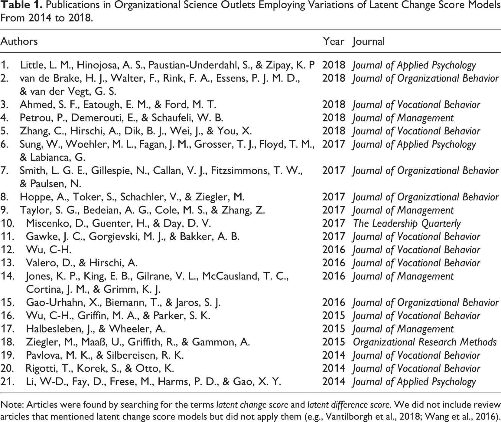
Note: Articles were found by searching for the terms latent change score and latent difference score. We did not include review articles that mentioned latent change score models but did not apply them (e.g., Vantilborgh et al., 2018; Wang et al., 2016).
As the method gained in popularity (see Figure 1), its name gradually evolved from latent difference score to latent change score modeling. This is because difference scores, in the traditional sense (e.g., xt – xt –1), have several shortcomings (Edwards, 2001), and thus often elicit adverse reactions, yet are never actually calculated in LCS models. Instead, change is represented by latent variables in LCS models. This name change also occurred because the term difference(s) is often used to discuss dissimilarities between units (e.g., individuals, teams) rather than change within units (Ferrer & McArdle, 2010). Although LCS models can be used to examine between-unit differences (e.g., Bernard et al., 2015), the basic, univariate LCS models that serve as the foundation for more complex, multivariate (e.g., bivariate), dynamic models capture the development that occurs within constructs within units over time (e.g., evolution in verbal ability within-individuals across their life spans).
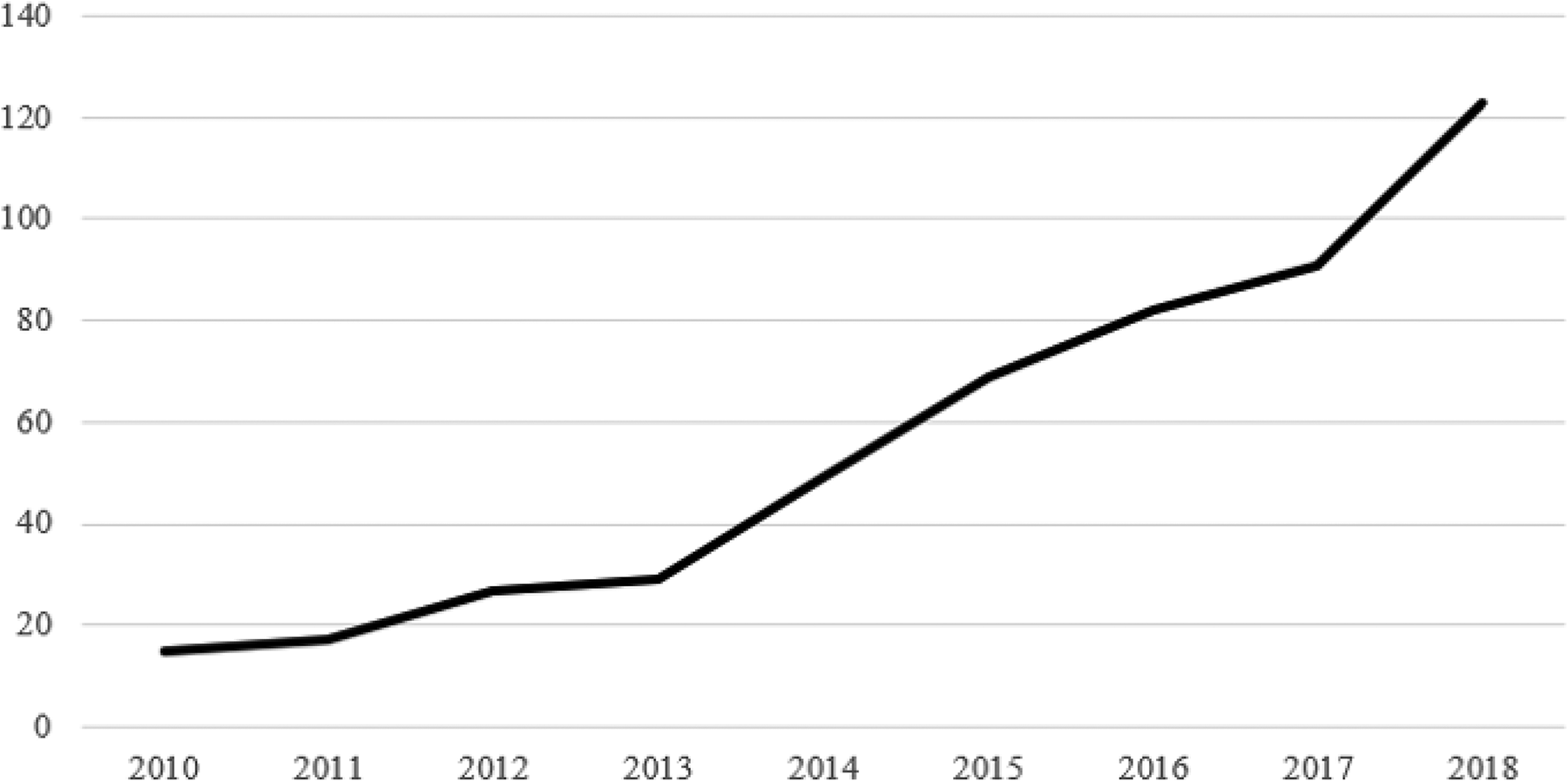
Number of articles, across disciplines, referencing latent change score models between 2010 and 2018.
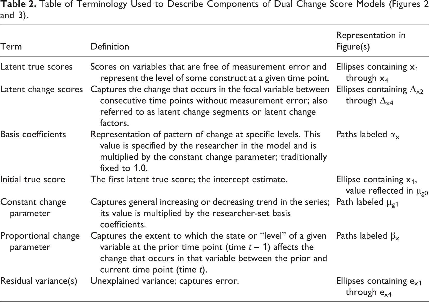
Indeed, univariate (i.e., single variable) LCS models essentially deconstruct the trajectory of a single variable into a sequence of latent true scores (i.e., scores on variables that are free of measurement error and represent the level of some construct at a given time point) and latent change scores, the latter of which captures the change that occurs in the focal variable between consecutive time points (also without measurement error). The latent true scores for variable x are represented by the ellipses containing x1 through x4 in Figures 2 and 3. The latent change scores (or latent change “factors,” as they are sometimes referred to; Clark et al., 2018) for variable x are represented by the ellipses containing Δx2 through Δx4 in Figures 2 and 3.
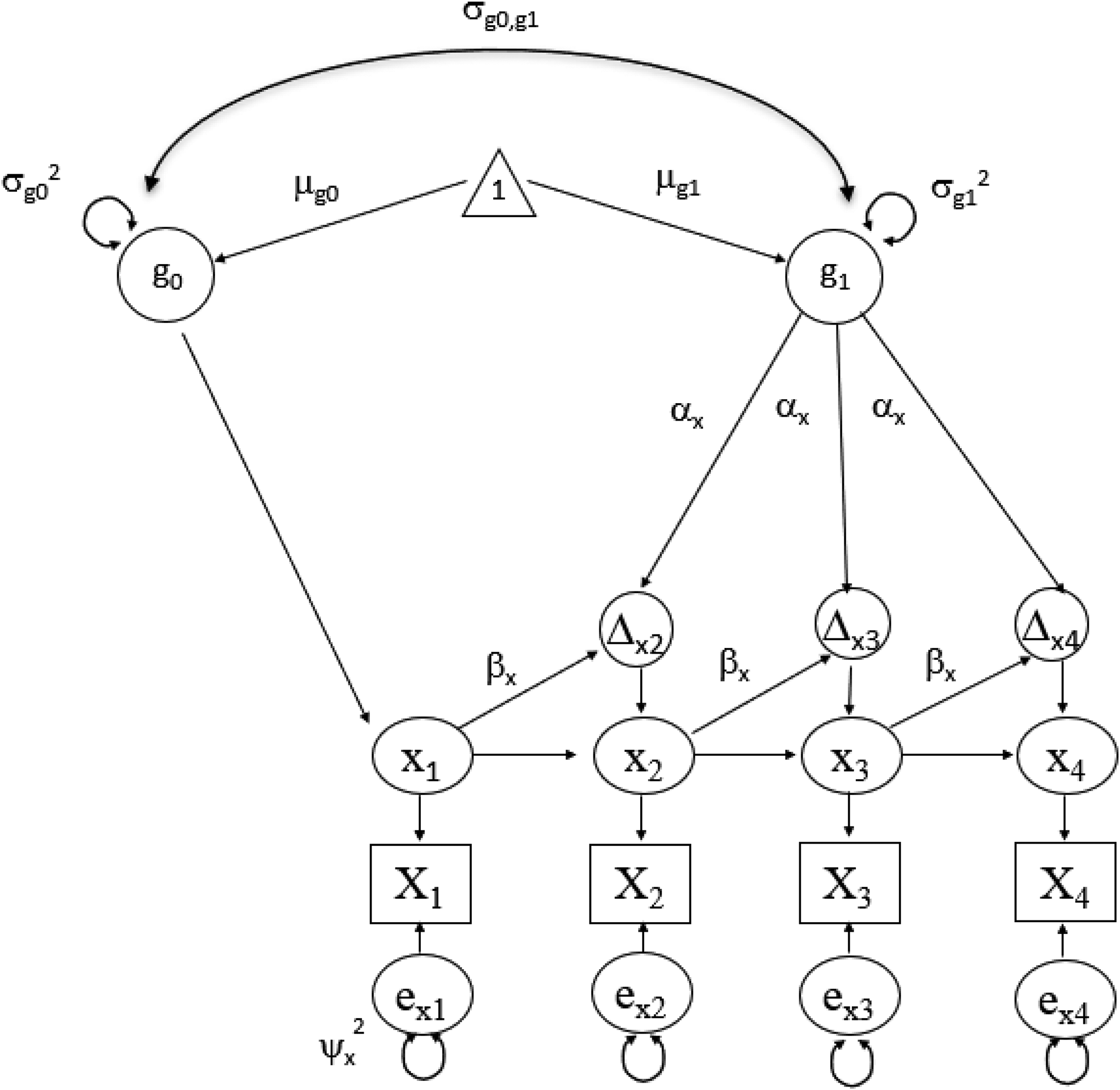
Univariate dual change score model with four time points.
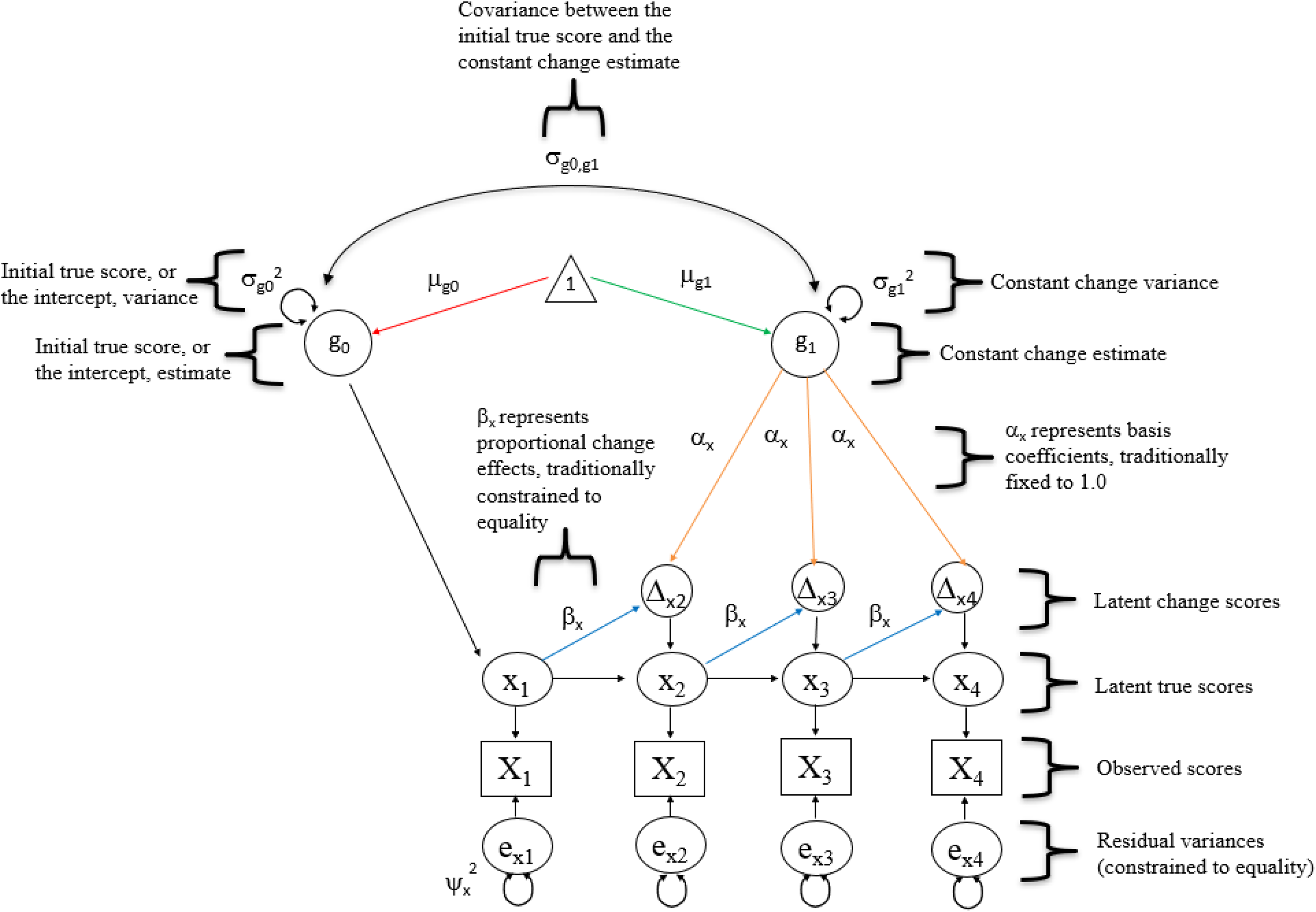
Univariate dual change score model with four time points, with annotated and highlighted paths.
Key Components of Dual Change Score Models: Proportional and Constant Change
Once modeled, latent change scores may be predicted by a variety of variables, including prior levels of the focal variable itself. For example, the univariate dual change score model, the most foundational LCS model and most commonly used basis for more complex, multivariate LCS models (Clark et al., 2018), predicts latent change using two distinct estimates derived from the variable itself. These estimates are captured by the proportional change and constant change parameters (Grimm et al., 2017). In Figures 2 and 3, βx represents the proportional change parameter estimate for variable x, and µg1 represents the constant change parameter estimate for variable x. Table 2 provides definitions for each of the components associated with dual change score models just discussed.
As it pertains to interpretation, the proportional change estimate does not reflect autoregression (also referred to as stability or memory; Barker et al., 2014). This can be a point of confusion for new users. In LCS models, the autoregressive weight of variable xt on variable xt –1 is actually fixed to 1.0, as is the loading for the latent change score factor reflecting the change that occurred in variable x between time t and time t – 1, in order to effectively mimic subtraction (Kievit et al., 2018). As explained by McArdle (2009), doing this results in a latent change score factor that “is now explicitly defined as ‘the part of the score of [variable xt ] that is not identical to [variable xt –1]’” (p. 583). Thus, LCS models account for autoregression, but they do not provide an explicit test of stability, unlike alternative models such as the autoregressive latent trajectory (ALT) model (Barker et al., 2014). We will discuss the ALT model as well as similar analytical approaches later in the article.
What the proportional change estimate does tell researchers is the direction and magnitude to which the state or “level” of a given variable at the prior time point (time t – 1) affects the change (Δ) that occurs in that variable between the prior and current time point (i.e., the change that occurs between time t – 1 and time t). That is, it informs researchers as to how much a variable’s score at time t – 1 is related to ensuing increases or decreases in that variable, if it is related whatsoever. For example, a significant, positive proportional change estimate in a univariate LCS model could provide evidence for the argument that newly hired employees with higher quality (or higher levels of) leader-member exchange (LMX) in one month (time t – 1) will exhibit larger increases in LMX by the next month (time t) relative to those employees who have lower quality LMX at time t – 1. As another example, a significant, negative proportional change estimate could provide evidence for the argument that employees with higher levels of commitment in one year (time t – 1) will exhibit larger decreases in commitment by the next year (time t) relative to employees who have lower levels of commitment at time t – 1.
In contrast to the proportional change estimate, the constant change estimate captures the general increasing or decreasing trend in the series. For example, a significant, negative constant change estimate in a model examining employee commitment might suggest that employees decreasingly commit to their organizations over time (although all parameter estimates should be considered jointly when plotting trajectories—more on this in the following). In this sense, the constant change estimate is akin to a slope factor in LGC models (Clark et al., 2018). In fact, LCS models that explicitly exclude proportional change estimates effectively operate as LGC models (Grimm, Castro-Schilo, & Davoudzadeh, 2013), specifically linear models given that the constant change estimate specifies that a fixed amount of change occurs over time. This is because the basis coefficients (labeled αx in Figures 2 and 3), which are multiplied by the constant change estimate when determining a variable’s overall trajectory (see Equation 1), are traditionally fixed to 1.0 across all time points.
Given their capabilities, widespread use, and principle role in more complex, multivariate models, dual change score models—the most foundational LCS model—will be the primary focus of this article henceforth. Although constant change and proportional change estimates may be omitted from univariate LCS models, the inherent value of the dual change score modeling approach comes from its ability to (a) capitalize on the strengths of two dominant analytical techniques (LGC and ARCL), (b) capture change over discrete intervals without difference scores, (c) provide empirical evidence that prior levels of a variable predict ensuing increases or decreases in that variable (i.e., proportional change), and (d) be extended to more complex, multivariate models examining dynamic construct relationships. We expand on each of these latter three strengths in the following.
Reliably Capture Change Over Discrete Intervals
First, the ability to model within-construct change without difference scores enables a plethora of research opportunities that existing approaches preclude. In dual change score models, the unique change that occurs between each time point is distinctly and reliably (in the psychometric sense) modeled. Thus, the latent variable representing the change that occurs in a construct between time t and time t + 1 is distinct from the latent variable representing the change that occurs in this same construct between time t + 1 and time t + 2, time t + 2 and time t + 3, and so forth. Each of these error-free, optimally reliable latent variables represents a potential outcome that can be explained or predicted by covariates (i.e., variables other than the prior level of the focal variable itself, which is captured by proportional change estimates; King et al., 2006). Although the parameter estimates of these covariates are frequently constrained to equality across change segments to help with model convergence, researchers may—and potentially should, depending on theory—allow these parameters to be freely estimated over time (we elaborate more on this later in the article).
As an example of one application, consider research that has demonstrated that extraversion is positively related to team-member-rated influence in the early stages of a group’s life cycle but is unrelated in the later stages of a group’s life cycle (Deuling et al., 2011). Assuming that one is interested in how extraversion affects changes in influence (i.e., increases or decreases) as the team continues to operate over time, one could regress each latent change score (i.e., change segment) on extraversion and allow this effect to be freely estimated for each. Such nuanced trajectories are almost unheard of in OPOB because dominant approaches for modeling longitudinal phenomena, such as LGC models, are unable to reliably capture change over discrete intervals (Grimm, Castro-Schilo, & Davoudzadeh, 2013). Instead, the primary objective of such methods is to describe general trajectories (Collins et al., 2016).
Provide Empirical Evidence of Past-Dependent, Proportional Change
A second strength of LCS models is that they allow researchers to empirically demonstrate that the starting point or prior level of a variable predicts subsequent increases or decreases in that variable. For example, Matusik, Hollenbeck, Matta, and Oh (2019) demonstrated with univariate models that teams who undergo the transition from standalone teams to component teams nested within multiteam systems experience decrements to their psychological empowerment. Furthermore, their findings suggest that standalone teams with “high” levels of psychological empowerment before the transition experienced greater decrements than those with “low” levels of psychological empowerment. Again, it is important to note that this is not autoregression. Rather, the proportional change estimates in dual change score models indicate whether and to what extent the level of a variable at time t predicts increases (indicated by a significant, positive proportional change coefficient) or decreases (indicated by a significant, negative proportional change coefficient) in that same variable. It does not indicate whether the level of a variable at time t is related to the level of that same variable at time t + 1.
A Basis for Dynamic Multivariate Models
A final strength of dual change score models is that multiple may be combined to examine dynamic, cross-lagged relationships among constructs. For example, the bivariate dual change score model, the most commonly fit bivariate LCS model, allows for “couplings” among constructs, or the ability to test whether constructs reciprocally influence one another over time (Grimm et al., 2017). That is, bivariate dual change score models not only quantify within-variable change (much like univariate dual change score models) but also occasion-to-occasion associations among variables. In this sense, bivariate dual change score models allow one to test whether variables have dynamic, mutually reinforcing relationships with one another over time, a possibility previously proposed by organizational scientists (e.g., Mitchell & James, 2001) that has only recently received testing in the literature.
Although the application of LCS models in organizational research is in its infancy, those researchers that have employed these models have often done so to examine reciprocal relationships between constructs. For example, Toker and Biron (2012) utilized a bivariate model to examine the temporal relationship between job burnout and depression. These researchers ultimately found that increases in depression were associated with subsequent increases in job burnout and vice versa. Similarly, Li and colleagues (2014) demonstrated that changes in work characteristics may lead to changes in personality and that changes in personality may also lead individuals to shape characteristics of their work down the road. As one final example, Taylor and colleagues (2017) examined a three-variable LCS model to test dynamic mediation.
While on the topic of the relationship between univariate and bivariate dual change score models, it is important to distinguish the concept of change from the concept of dynamics. We construe the concept of change as simply the development that occurs in a single variable. This development might occur over a discrete interval (e.g., the difference in variable x between time t and time t – 1) or across an entire window of observation (i.e., the overall trajectory a variable exhibits, the focus of LGC models). Univariate dual change score models solely capture change through (a) modeling the overall trajectory of a variable, (b) decomposing that trajectory into discrete change segments, and (c) estimating proportional (past-dependent) change. Thus, researchers might use univariate dual change score models if their research questions pertain to trajectories, proportional change, or the specific amount of change that occurs between measurement occasions. However, these models do not directly speak to dynamics.
Although some organizational researchers have equated autoregression with dynamics (see Dishop et al., 2020, p. 417, for examples of this in the literature), this is inconsistent with how we conceptualize dynamics and how dynamics are conceptualized by other scientific disciplines (e.g., physics, biology; Xu et al., 2020). Generally speaking, other disciplines would consider two variables to be dynamic (or would argue that they share a dynamic relationship) if there are significant cross-lagged relationships among them (i.e., variable x at time t predicts change in variable y at time t + 1 and vice versa). For example, the autoregressive distributed lag (ARDL) model is a dynamic model because it examines the concurrent (i.e., time t) and cross-lagged (i.e., time t – 1) effects of variable x on variable y at time t (and accounts for autoregression in variable y in doing so; Xu et al., 2020). Consistent with Xu et al. (2020), as well as other scientific disciplines, we consider dynamic models to be those that examine cross-lagged relationships between variables, and we do not equate the term dynamics with autoregression. Although bivariate dual change score models indeed capture change and account for autoregression like univariate dual change score models, they differ from univariate models in that they may be used to examine dynamic relations among two variables.
In sum, there are a number of strengths associated with this methodology. LCS models, and particularly dual change score models, capitalize on the strengths of both LGC and ARCL models. They also allow researchers to model and predict change over discrete intervals in an optimally reliable way, enabling the exploration of nuanced developmental trajectories. Finally, these models allow researchers to test proportional change in constructs of interest and may be expanded to multivariate models that enable investigations into complex, dynamic relationships among two or more constructs. With these strengths in mind, we next turn to modeling procedures, focusing first on the univariate dual change score model before transitioning to more complex, multivariate LCS models.
Dual Change Score Modeling Procedures
In this section, we walk readers through modeling procedures for univariate and bivariate dual change score models. We provide a running example with real data, specifically the first four years of data collected as part of the LISS (Longitudinal Internet Studies for the Social sciences) panel administered by CentERdata (Tilburg University, The Netherlands), which is freely available to researchers on request (see https://www.lissdata.nl/). We chose to use these data because there are equal intervals between measurement occasions (1 year; see Best Practice 1 in the Discussion section) and because it provides a more than sufficient sample size (n = 9,402), per our power analysis (see Best Practice 2 in the Discussion section). Readers can find the syntax for all models discussed in this article’s GitHub repository (https://github.com/researcher2653/lcsorm).
For our running example, we focus on life satisfaction and pay satisfaction because the two may share a mutually reinforcing, reciprocal relationship. Greater satisfaction with one’s pay may be associated with subsequent increases in one’s general satisfaction with life, and greater general life satisfaction may “spill over” and positively influence one’s satisfaction with one’s pay. Both constructs were measured with a single item (“We would first like to know how satisfied you are with your wages or salary or profit earnings” and “How satisfied are you with the life you lead at the moment?”) and on an 11-point scale (0 = not at all satisfied, 10 = fully satisfied or completely satisfied). Furthermore, we linearly transformed participants’ responses by adding 1 to each (thus avoiding responses with a value of 0), and we used full-information maximum likelihood (FIML) estimation to handle missing data (per Best Practice 3 in the Discussion). 1
Univariate Dual Change Score Models
The unconditional, univariate dual change score model may be described as a nested (or hierarchical; Kline, 2011) model. Nested within the univariate dual change score model is the univariate intercept-only (or “no change”) model and the univariate constant change model (akin to a linear LGC model). In what follows, we describe the typical parameters that are freely estimated in each of these models. It is important to note that some model specifications may be relaxed (e.g., equality constraints), which we discuss in a later section.
The intercept-only model provides information about a construct’s starting point (or intercept). It typically contains three freely estimated parameters: the intercept mean/estimate, the intercept variance, and the residual variance, which is constrained to equality across measurement occasions (i.e., a single estimate represents all residual variances). This model is nested within the constant change model. The constant change model provides information about the construct’s starting point (or intercept) and its general pattern of change (positive or negative). It typically contains six freely estimated parameters: all of those in the intercept-only model as well as the constant change mean/estimate, the constant change variance, and the covariance between the constant change parameter and intercept. This model is nested within the dual change score model. Finally, the dual change score model provides information regarding the construct’s starting point, general pattern of change, and proportional change. It typically contains seven freely estimated parameters: all of those estimated in the constant change model as well as a proportional change estimate. The proportional change estimate is usually constrained to equality across latent change score factors, thus resulting in a single estimate representing all proportional change (Clark et al., 2018). 2
Thus, to build a dual change score model, we start by constructing the entire model and constraining the parameters associated with the higher-order constant change and dual change score models to zero (see the “Intercept-Only Model” code in the GitHub repository). This gives us the model fit statistics and three parameter estimates for the intercept-only model. Then, we relax the constraints on the parameters associated with the constant change model because the intercept-only model is nested within the constant change model (see the “Constant Change Model” code in the GitHub repository). This gives us the model fit statistics and six parameter estimates for the constant change model. Assuming the results of a chi-square difference test suggest that the more complex, constant change model provides a significant improvement in fit over the intercept-only model, we can then relax the constraints placed on the proportional change estimates (see the “Univariate Dual Change Score Model” code in the GitHub repository). This gives us the model fit statistics and seven parameter estimates for the dual change score model. We then, again, conduct a chi-square difference test to determine whether there is a significant improvement in model fit.
The dual change score model may be retained if it (a) provides a significant improvement in model fit over the constant change model and (b) meets commonly accepted standards for acceptable fit based on indices familiar to organizational researchers such as root mean square error of approximation (RMSEA), comparative fit index (CFI), and standardized root-mean-square residual (SRMR; Bentler, 1990; Hu & Bentler, 1999; Kline, 2011). Moreover, the choice to retain the dual change score model should be informed by theory rather than justified post hoc (i.e., “harking,” or hypothesizing after results are known; Bosco et al., 2016). That said, we recognize that the nuance and complexity of the theories currently in place are often overmatched relative to the nuance and complexity of the potential empirical models that can be tested via LCS modeling. Thus, the value of LCS models as a transparently employed, inductive theory-building tool cannot be overestimated (Hollenbeck & Wright, 2017; Vancouver, 2018).
Once a model is selected (based on the requisites outlined previously), significant (p < .05) parameter estimates may be interpreted. The interpretation of the mean of the intercept (also referred to as the initial true score) is relatively straightforward because it represents the predicted average starting point of the construct under consideration. However, the interpretations of the constant change and proportional change parameters are more complex because they conjointly shape the overall trajectory of the focal construct. As noted previously, a positive constant change estimate typically suggests a general increasing trend, and a negative constant change estimate typically suggests a general decreasing trend. As also noted, a positive proportional change estimate suggests that the value (or state) of the construct at time t is related to ensuing increases between time t and time t + 1, and a negative proportional change estimate suggests that the value (or state) of the construct at time t is related to ensuing decreases between time t and time t + 1.
However, researchers must take all three estimated parameters (i.e., the intercept, constant change, and proportional change estimates) together when plotting overall trends. This can be accomplished by using the following equation:

where Δxt+1 represents the average amount of change that occurs in variable x between time t and time t + 1, µ x represents the model-estimated constant change parameter, α x represents the researcher-set basis coefficient (which is typically fixed to 1.0), β x represents the model-estimated proportional change parameter, and x t represents the value of the latent true score for variable x at the prior (or perhaps initial) point in time. Assuming that xt is the intercept (i.e., the initial true score, or first time point), the value ultimately calculated for Δ x t +1 is added to the intercept estimate provided by the dual change score model to derive the estimate for the latent true score for the second time point (time t + 1 in this example). Then the process repeats, with the latent true score derived for Time 2 (time t + 1) feeding into the next change estimate and, consequently, latent true score for Time 3 (time t + 2 in this example).
To illustrate this process, we will examine pay satisfaction and life satisfaction using the first 4 years of the LISS data set (as noted). Again, sample syntax can be found in the GitHub repository. The intercept-only model for pay satisfaction did not provide an acceptable fit, χ2(11) = 278.99, p < .01, CFI = .93, RMSEA = .06, SRMR = .10, based on the SRMR estimate. 3 The constant change model, χ2(8) = 113.25, p < .01, CFI = .97, RMSEA = .05, SRMR = .04, and dual change score model, χ2(7) = 72.43, p < .01, CFI = .98, RMSEA = .04, SRMR = .05, both provided acceptable fit. To determine whether the more complex, higher-order models provided significant improvements in fit over the simpler, lower-order models, we engaged in a series of chi-square difference tests. These tests revealed that the constant change model provided a significant improvement in fit over the intercept-only model, χ2 diff(3) = 165.74, p < .01, and that the dual change score model provided a significant improvement in fit over the constant change model, χ2 diff(1) = 40.82, p < .01. Thus, the dual change score model was retained.
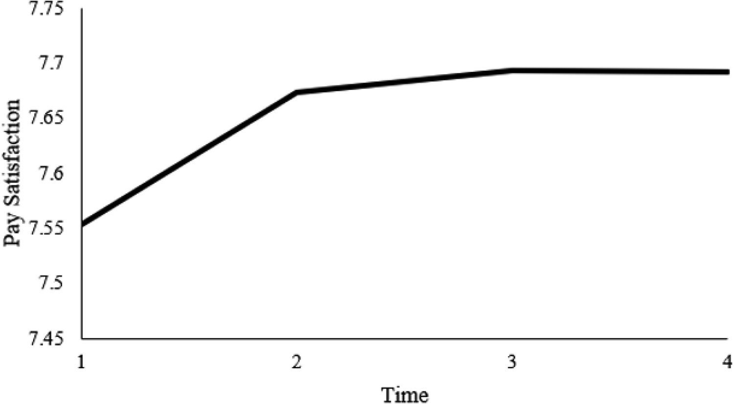
The dual change score model provided an intercept estimate of 7.584 (p < .01), a constant change estimate of 3.996 (p < .01), and a proportional change estimate of –.515 (p < .01), and we fixed our basis coefficients to 1.0 (as is typical for these models). The results suggest that participants’ pay satisfaction averaged 7.584 at the start of the study (equivalent to the intercept estimate) and increased, on average, by .090 by the second measurement (3.996 + [–.515 × 7.584]), .044 by the third measurement (3.996 + [–.515 × 7.674]), and .021 by the fourth measurement (3.996 + [–.515 × 7.718]). These results also suggest that despite a general upward trend in terms of pay satisfaction, pay satisfaction increased at a decelerating rate over time. This reduced rate is due to the fact that the proportional change estimate (–.515) is multiplied by a larger value at each successive time point because scores increase, on average, over time. That is, because pay satisfaction increases between measurement intervals, the effect of the proportional change estimate strengthens with time. This is why dual change score models are considered to be nonlinear, cumulative models (McArdle & Nesselroade, 2014). The second occasion accounts for the first occasion, the third occasion accounts for the second occasion, and so on and so forth, ultimately resulting in a curvilinear trend (see Figure 6 for pay satisfaction). A tool for plotting these trajectories can be found in this article’s GitHub repository.
Interestingly, a different pattern emerged when examining life satisfaction. The intercept-only, χ2(11) = 206.27, p < .01, CFI = .98, RMSEA = .05, SRMR = .04; constant change, χ2(8) = 86.06, p < .01, CFI = .99, RMSEA = .03, SRMR = .06; and dual change score, χ2(7) = 33.38, p < .01, CFI = 1.0, RMSEA = .02, SRMR = .05, models all provided acceptable fit. Additionally, a series of chi-square difference tests revealed that the constant change model provided a significant improvement in fit over the intercept-only model, χ2 diff(3) = 120.21, p < .01, and that the dual change score model provided a significant improvement in fit over the constant change model, χ2 diff(1) = 52.68, p < .01. Thus, the dual change score model was retained.
The dual change score model provided an intercept estimate of 8.556 (p < .01), a constant change estimate of 5.894 (p < .01), and a proportional change estimate of –.698 (p < .01), and we fixed our basis coefficients to 1.0. These results suggest that participants’ life satisfaction averaged 8.556 at the start of the study (equivalent to the intercept estimate) and decreased, on average, by .08 by the second measurement (5.894 + [–.698 × 8.556]), .022 by the third measurement (5.894 + [–.698 × 8.476]), and .01 by the fourth measurement (5.894 + [–.698 × 8.454]). These results also suggest that despite a general downward trend, life satisfaction declined at a slower rate over time (see Figure 7). This reduced rate is due to the fact that the proportional change estimate (–.698) is multiplied by a smaller value at each successive time point because scores decrease, on average, over time. That is, because life satisfaction decreases between intervals, the effect of the proportional change estimate weakened with time.
As noted previously, researchers should be aware that although the univariate intercept-only, constant change, and dual change score models “typically” have three, six, and seven freely estimated parameters (respectively), residual variances and proportional change estimates do not necessarily need to be constrained to equality over time. They are usually constrained to equality to facilitate model convergence and conserve degrees of freedom. If researchers find that models do not converge with equality constraints or if there is a theoretical reason to assume residual variances and/or proportional change estimates vary over time, then these homogeneity assumptions may be relaxed (see Best Practice 6). Researchers should follow the hierarchical model testing procedures described previously if equality constraints are relaxed, and chi-square difference tests should be used to determine which model to retain.
Bivariate Dual Change Score Models
As noted, another major objective of LCS models is to examine time-sequential associations (or dynamic “couplings,” or cross-lagged relationships) between constructs. Researchers may use the bivariate dual change score model to estimate such associations. An examination of Figures 4 and 5 reveals that the bivariate dual change score model is simply two univariate dual change score models with associations among the constructs’ latent true and latent change scores, slopes, and intercepts. Specifically, γ y represents the effect of variable x’s latent true score at time t on the change that occurs in variable y between time t and time t + 1, and γ x represents the effect of variable y’s latent true score at time t on the change that occurs in variable x between time t and time t + 1.
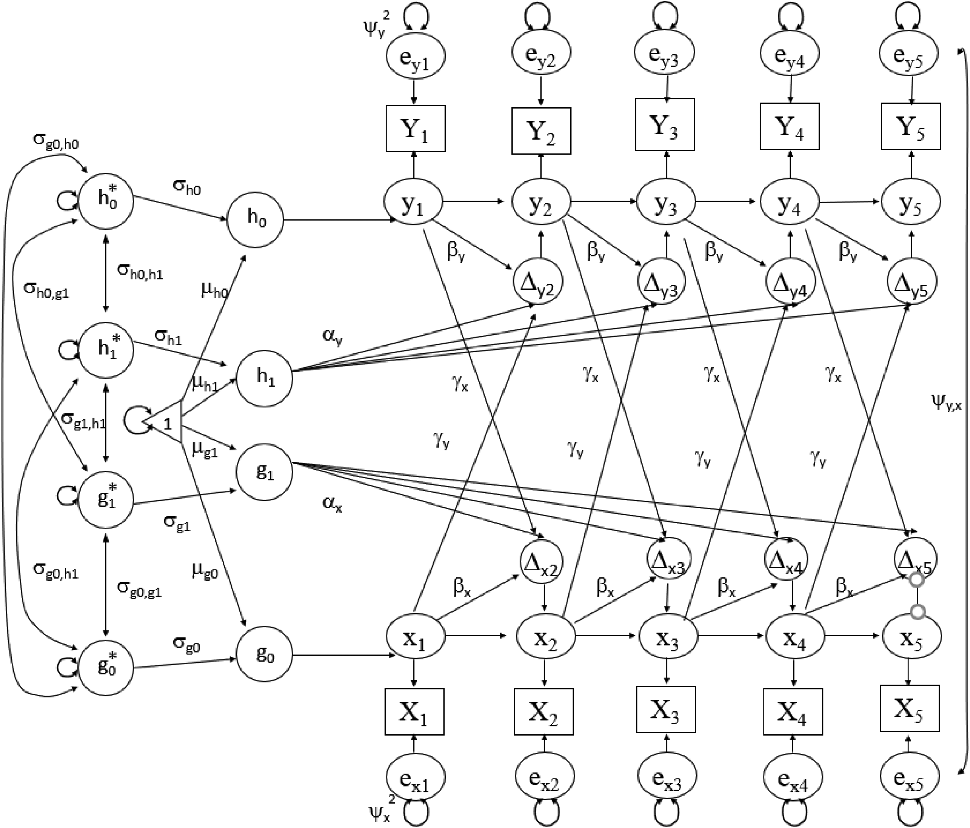
Bivariate dual change score model with five time points.
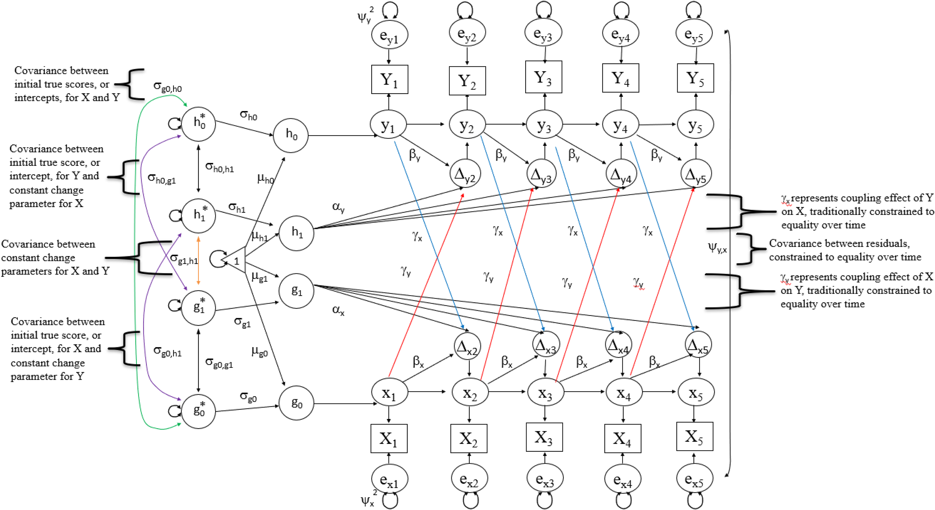
Bivariate dual change score model with five time points, with annotated and highlighted paths.
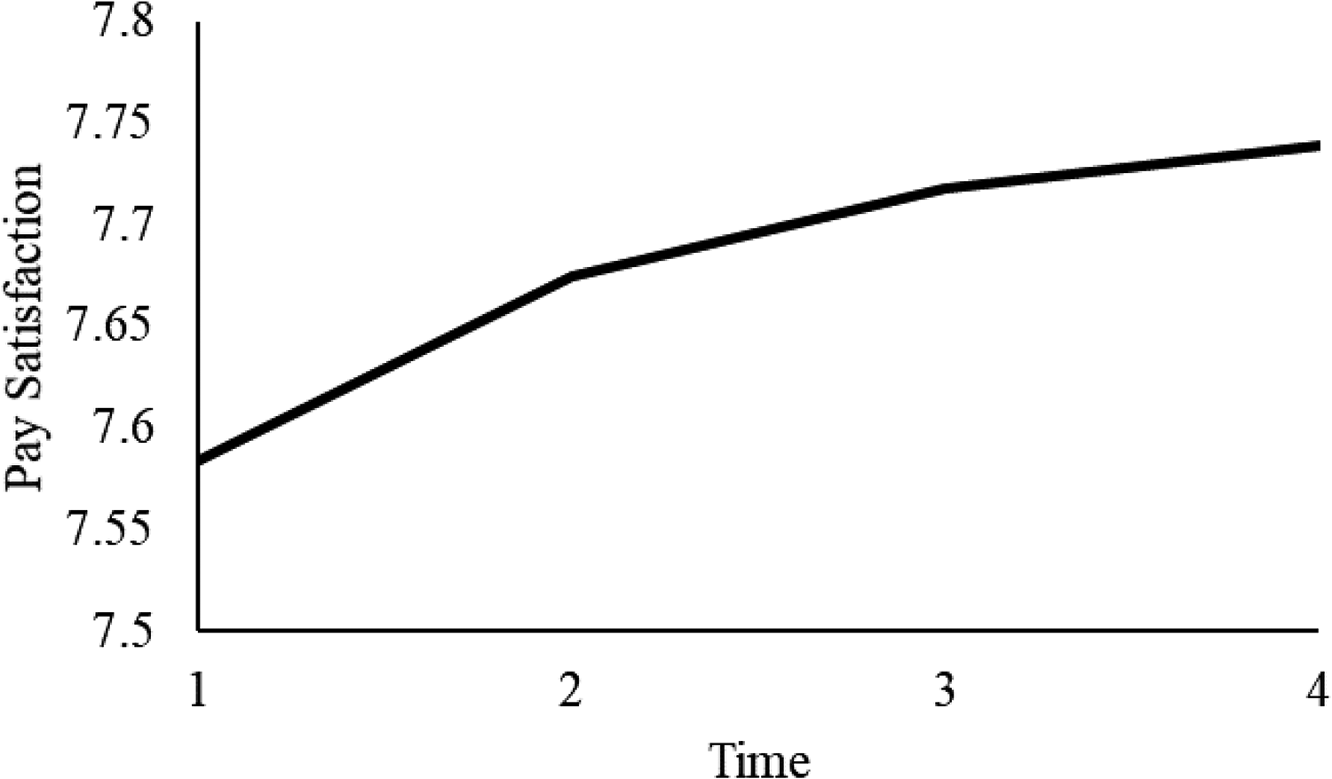
Univariate dual change score model trajectory for pay satisfaction.
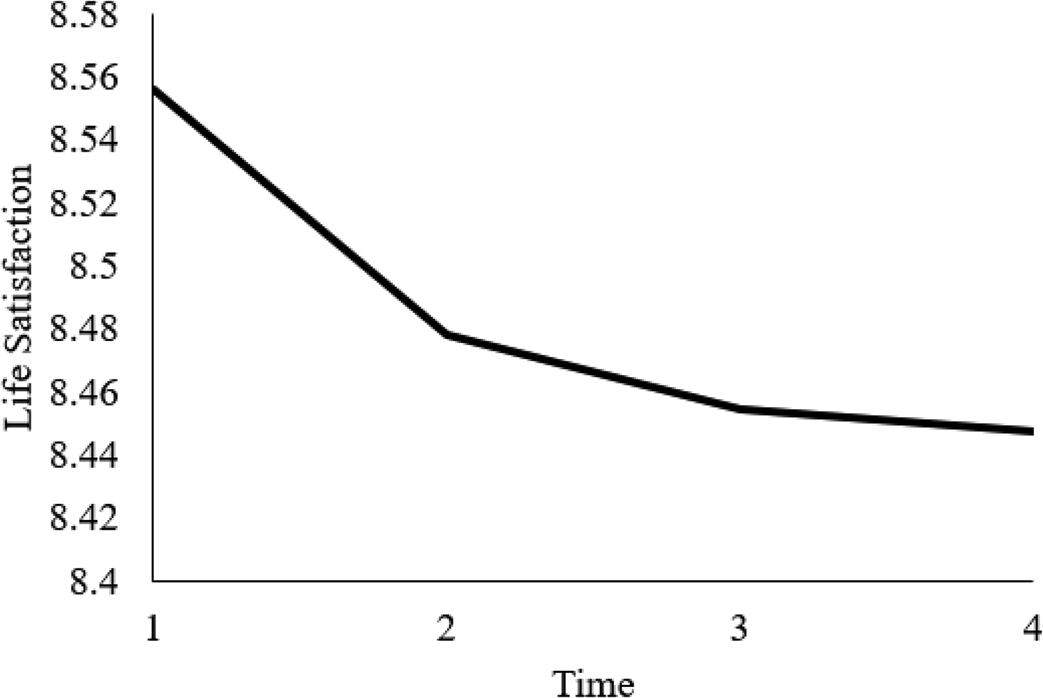
Univariate dual change score model trajectory for life satisfaction.
The unconditional, bivariate dual change score model may be described as nested (or hierarchical; Kline, 2011) like the univariate dual change score model. Typically, a series of four bivariate dual change score models are fit in determining whether two variables have time-sequential associations with one another (Grimm et al., 2017), although researchers may choose to engage in more rigorous tests of nesting. We advise running univariate models for the two constructs of interest before running the bivariate model to ensure that dual change score models are appropriate for the data. However, we realize that this is a more “purist” approach that some researchers adhere to (e.g., Hounkpatin, Boyce, Dunn, & Wood, 2018) and others do not (e.g., Ferrer et al., 2007). Considering that a series of four nested models is the norm, we focus on this approach (see the “Bivariate Dual Change Score Model” code in the GitHub repository).
In the first of the four models (the “no coupling” model), all coupling parameters (γ y and γ x ) are constrained to zero, indicating no time-sequential associations among variables. In the second and third models, unidirectional couplings are fit. That is, in one of these models, the effect of variable x on variable y (γ y ) is estimated while the effect of y on x (γ x ) is constrained to zero, and in the other model, the effect of y on x (γ x ) is estimated while the effect of x on y (γ y ) is constrained to zero. As is the case with the proportional change estimates in the univariate dual change score model, the estimated coupling effects are typically constrained to equality over time (e.g., the coupling effect of x on y, or γ y , is held constant over time). Therefore, these models result in the estimation of one additional parameter and the loss of one degree of freedom over the no coupling model. In the fourth and final model (the “full coupling” model), the simultaneous effects of the two variables on one another are freely estimated (i.e., both γ y and γ x are freely estimated). As before, these parameters are usually constrained to equality over time (e.g., γ y between time t and time t + 1 is assumed to be equal to γ y between time t + 1 and time t + 2). To clarify, however, they are not held constant to one another (i.e., γ y is not constrained to the same value as γ x ). Therefore, the resultant, full coupling model should provide two additional parameter estimates over the no coupling model and have two fewer degrees of freedom.
Given their nested nature, researchers should engage in a series of chi-square difference tests to ensure that the added complexity of higher-order models is warranted. Assuming that (a) these tests suggest that a higher-order model is justified and (b) this model provides acceptable fit statistics, researchers may then interpret significant parameter estimates. For example, a negative, significant coupling effect of variable x on variable y suggests that higher values of the latent true score x at time t are associated with subsequent decreases in y between time t and time t + 1. Once again, however, researchers must take all model estimates (intercept, constant change, proportional change, and couplings) into account when plotting trajectories. This may be accomplished through a simple extension of Equation 1, from the prior section:

For variable x, where Δ x t +1, µ x , α x , β x , and xt have the same interpretation as before, γ x represents the coupling effect variable y has on variable x, and yt is the value of the latent true score for variable y at the prior (or perhaps initial) point in time (time t). A simple adaptation of this formula can be made to calculate change in variable y:

Just as before, the results of these formulas (Δ x t +1 and Δ y t +1) represent the change that occurs between time points, and this change is added to the prior time point (xt and yt , respectively) to acquire the value for the subsequent time point (xt +1 and yt +1). Furthermore, these resultant values are reentered into their respective formulas to calculate Δ x t +2 and Δ y t +2 because these models are cumulative (McArdle & Nesselroade, 2014).
To illustrate this process, we return to our running example of pay satisfaction and life satisfaction. Say that we hypothesize a dynamic, reciprocal relationship between the two such that they are mutually reinforcing: Higher levels of pay satisfaction will be related to subsequent increases in life satisfaction and vice versa. The first model, the no coupling model, provided an acceptable fit to the data, χ2(25) = 122.03, p < .01, CFI = .99, RMSEA = .02, SRMR = .04. Our first unidirectional coupling model, in which the effects of life satisfaction on changes in pay satisfaction were freely estimated, also provided an acceptable fit, χ2(24) = 116.32, p < .01, CFI = .99, RMSEA = .02, SRMR = .04, and a significant improvement in fit over the no coupling model, χ2 diff(1) = 5.71, p = .02. Our second unidirectional coupling model, in which the effects of pay satisfaction on changes in life satisfaction were freely estimated, provided an acceptable model fit, χ2(24) = 120.55, p < .01, CFI = .99, RMSEA = .02, SRMR = .04, but did not provide a significant improvement in model fit over the no coupling model, χ2 diff(1) = 1.48, p = .22. Finally, the full coupling model provided an acceptable fit to the data, χ2(23) = 115.13, p < .01, CFI = .99, RMSEA = .02, SRMR = .04, and a significant improvement in fit over the no coupling model, χ2 diff(2) = 6.90, p = .03, but not over our first unidirectional coupling model, χ2 diff(1) = 1.19, p = .27. Thus, the unidirectional coupling model, in which the effects of life satisfaction on changes in pay satisfaction were freely estimated, was retained.
The results of our retained model included a positive and significant intercept estimate for pay satisfaction (B = 7.554, p < .01), a positive but nonsignificant constant change estimate for pay satisfaction (B = 0.785, p = .596), a negative and significant proportional change estimate for pay satisfaction (B = –0.547, p < .01), and a positive and significant coupling estimate for the effect of life satisfaction on pay satisfaction (B = 0.405, p = .02). These results suggest that (a) there is a general upward, nonlinear trend in pay satisfaction; (b) prior scores on assessments of pay satisfaction act as a limiting factor on subsequent increases in pay satisfaction (as was the case in our univariate model); and (c) prior scores on assessments of life satisfaction act as a facilitating factor (or a positive leading indicator) on subsequent increases in pay satisfaction. These results lend some support to our hypothesis, specifically our argument that higher levels of life satisfaction spill over and lead to increases in pay satisfaction.
However, the retained model did not include a significant coupling effect of pay satisfaction on life satisfaction. This suggests that pay satisfaction is not a leading indicator of subsequent changes in life satisfaction. That is, the latent true score for pay satisfaction at time t does not positively or negatively affect the change that occurs in life satisfaction between time t and time t + 1. Thus, life satisfaction and pay satisfaction are not mutually reinforcing—although life satisfaction is associated with increases in pay satisfaction, pay satisfaction is not associated with increases in life satisfaction. Therefore, our hypothesis is only partially supported.
This trajectory for pay satisfaction is plotted in Figure 8 (the tool for which can be found in the GitHub repository). It should be noted that plotting bivariate dual change score models can also be completed with statistical vector plots, which is a complex technique that we do not believe is accessible or intuitive for the average user, both from a modeling and an interpretation standpoint. For those interested in learning more, however, we suggest reviewing work by Boker and McArdle (1995) as well as Z. Zhang et al. (2015).
Bivariate Dual change score model trajectory for pay satisfaction with unidirectional coupling effects.
Alternative Dual Change Score Models
As alluded to, these models can be made increasingly complex. For example, McArdle and Grimm (2010) discussed the use of multigroup bivariate dual change score models, which can be used to determine if there are between-group differences in dynamic couplings among constructs of interest. Although an in-depth discussion of multigroup modeling is beyond the scope of this article (the authors of this article may be contacted for syntax and instructions, if desired), researchers can test for between-group differences by initially specifying a model in which all parameter estimates are constrained to equality between Group A (e.g., males, or firms in turbulent industries, or subordinates, or employed individuals) and Group B (e.g., females, or firms in stable industries, or supervisors, or unemployed individuals) before slowly releasing these equality constraints. Researchers would then test whether allowing these estimates (means, variances, covariances, etc.) to be freely estimated significantly improves model fit. If there is a significant improvement in model fit, then it may be inferred that there are significant between-group differences in the freely estimated parameters.
Dual change score models may also be extended by including time-varying or time-invariant covariates predicting the various latent variables modeled in dual change score models (e.g., the moderating effect of physical activity on the temporal relationship between job burnout and depression; Toker & Biron, 2012). Moreover, they can be used to examine dynamic, longitudinal mediation (Simone & Lockhart, 2019), or the effect that change in some independent variable has on the change that occurs in a dependent variable, via the effect it has on the change that occurs in some mediating variable. For example, Taylor and colleagues (2017) examined the effect of changes in workplace incivility (time t – 1) on changes in turnover cognitions (time t + 1), via changes in burnout (time t), in a “trivariate” LCS model. As one final example of how these models may be extended, burgeoning research is finding that there may be value in examining dual change score models with curvilinear bases (e.g., quadratic dual change score models with basis coefficients fixed to values other than 1; Hamagami & McArdle, 2019).
Choosing Between LCS Models and Alternative Models
Until now, we have focused almost exclusively on LCS models. Although we have mentioned other modeling approaches in passing, we have not discussed alternative approaches to modeling longitudinal phenomena in great detail to avoid creating confusion in our exposition. This may leave researchers wondering whether LCS models are really the best methodological choice for their specific research questions or if alternative models might be equally (or even more) appropriate. In this section, we compare LCS models to other approaches that are commonly used to study longitudinal phenomena and share conceptual overlap with LCS models. These include latent growth curve models, autoregressive cross-lagged models, autoregressive distributed lag models, and autoregressive latent trajectory models. In Table 3, we include a high-level overview of the differences between these models. Also, we preface this section by stating that we are comparing the baseline, bivariate versions of these models to one another—we will not go into every variation of or modification that can be made to each of these models for the sake of space and clarity.
Comparison of Latent Change Score Models With Alternative Methods for Analyzing Longitudinal Data.
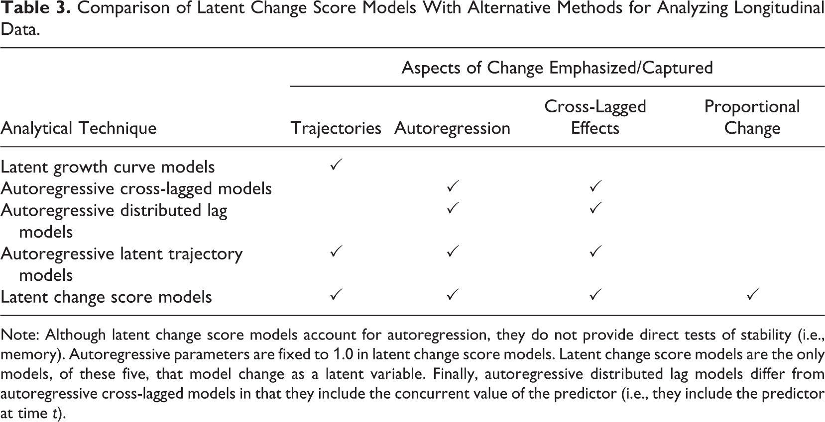
Note: Although latent change score models account for autoregression, they do not provide direct tests of stability (i.e., memory). Autoregressive parameters are fixed to 1.0 in latent change score models. Latent change score models are the only models, of these five, that model change as a latent variable. Finally, autoregressive distributed lag models differ from autoregressive cross-lagged models in that they include the concurrent value of the predictor (i.e., they include the predictor at time t).
We chose to focus on LGC, ARCL, ARDL, and ALT models not only because they are used to examine longitudinal phenomena but also because they are all based on the SEM framework (Barker et al., 2014; Hounkpatin et al., 2018). These models differ, however, in terms of the aspects of change they emphasize. Their emphasis may be on one or more of the following: (a) overall developmental processes, or overall change (i.e., trajectories); (b) autoregressive effects (i.e., stability, memory, self-similarity), or the effect that variable x at time t has on variable x at time t + 1; (c) cross-lagged effects (i.e., dynamic couplings), or the effect that variable x at time t has on variable y at time t + 1 (and vice versa); and (d) proportional change effects, or the direction and magnitude of the effect that variable x at time t has on the change (Δ) that occurs in variable x between time t and time t + 1.
The emphasis of baseline bivariate LGC models is on overall developmental processes, and thus trajectories, through the estimation of intercepts (i.e., initial values) and slopes (which are also referred to as mean-level change scores). Although one can examine covariances among intercepts and slopes, these models are not used to examine autoregressive, cross-lagged, or proportional change effects. Conversely, the emphasis of baseline bivariate ARCL models is on autoregressive and cross-lagged effects. They are like LGC models in that they are not used to examine proportional change, but they are unlike LGC models in that they do not explicitly model overall developmental processes (i.e., they do not capture slopes).
The emphasis of baseline bivariate ARDL models is also on autoregressive and cross-lagged effects, making ARDL models similar to ARCL models. Whereas ARCL models examine the effects of variable x and variable y at time t – 1 on variable y at time t (capturing cross-lagged and autoregressive effects, respectively), ARDL models examine these effects in addition to the concurrent (i.e., time t) effects of variable x on variable y at time t. An inspection of the formulas (p. 340) and figure (p. 341) explaining ARCL models, provided by Bollen and Curran (2004), and their comparison to the formula and figure (p. 598) provided by Xu and colleagues (2020) reveals the similarities between these two modeling approaches.
The baseline bivariate ALT model is most similar to the bivariate LCS model in that it combines aspects of both the LGC and ARCL models (Bollen & Curran, 2004). Thus, the emphasis of ALT models is on developmental processes, autoregression, and cross-lagged effects. However, ALT models do not explicitly model change between consecutive waves as a latent variable/factor, and relatedly, they do not capture proportional change. The baseline bivariate LCS model captures underlying developmental processes, autoregression, cross-lagged effects, and proportional change effects. Unlike ALT models, they explicitly model change as a latent variable, and, therefore, they can be used to treat change itself as a variable of theoretical interest. This is something that baseline ALT models (and all other models discussed) do not do.
In terms of choosing which method is the “right” one, we would personally advise against the use of baseline LGC and ARCL models. By ignoring autoregression and cross-lagged effects (LGC models) and overall development/trajectories (ARCL models), these models fail to fully flesh out the change that occurs in variables. Again, it is our personal belief that researchers avoid these techniques, although we can imagine one making the case that LGC models, for example, are sufficient if one is only interested in overall trajectories.
As noted, the key difference between ALT and LCS models is that ALT models do not model change as a latent variable. Thus, ALT models do not provide direct estimates of the change that occurs, and they cannot be used to predict interunit differences or variability in change. They also do not allow researchers to use change as a predictor of outcomes (e.g., change in one variable predicting change in another). Conversely, LCS models explicitly model change as a latent variable and thus can be used to divide trajectories into multiple discrete change segments, each of which is a potential outcome to be predicted or a potential predictor of other outcomes (King et al., 2006). They also capture proportional change effects and can be used to examine how change in one variable relates to changes in another variable, rather than how levels of one variable relate to levels/change in another variable. This latter strength of LCS models represents an important advantage over alternative approaches. Through modeling intraunit change (whereby change is predicated on prior levels within-units), researchers may be able to account for omitted interunit differences (e.g., ethnicity, gender) in variables that could act as confounds of the relationship between the variables of interest (Hounkpatin et al., 2018).
Ultimately, the goals of one’s research should determine model selection. If one is interested in examining the dynamic relations between two variables and is not interested in examining change (Δ) itself as a variable of interest, ALT models may suffice. Also, if one is interested in directly testing stability, one should not use LCS models because autoregressive parameters are fixed to 1.0 in these models. However, if one is interested in change as a theoretical variable, LCS models are preferred. In fact, Bollen and Curran (2004), in their article introducing ALT models, noted that “a researcher interested in studying change in a latent variable might prefer latent difference scores” (p. 376) over ALT models. Although LCS models are a bit more complex than ALT models (Barker et al., 2014), they allow for a greater breadth of research questions pertaining to change.
Discussion
One of our greatest qualities as a field is the eagerness with which we adopt new methodologies. After all, our “methods and measures are what make us a science” (Salas et al., 2017, p. 590). This said, and perhaps ironically, one of our greatest downfalls as a field is that we frequently apply methods incorrectly because we use them without fulling understanding them (Cortina, Aguinis, & DeShon, 2017). For example, a recent review of studies (a) published in top journals, (b) utilizing SEM, (c) reporting degrees of freedom in their results (as researchers always should), and (d) providing the information necessary for the reader to compute degrees of freedom themselves revealed that reader-computed degrees of freedom matched reported degrees of freedom only 62% of the time (Cortina, Green, et al., 2017). This suggests that the models tested in a significant portion of published articles are inconsistent with the theoretical models put forth by authors, seriously limiting the inferences that may be drawn from these analyses. As another example, an investigation on small sample mediation testing via bootstrapping, also common in top journals, revealed that this practice is associated with insufficient statistical power and may inflate one’s Type I error rate (Koopman et al., 2015).
The seriousness of these problems cannot be overstated, but they are the fault of the scientist and not the science. To avoid a similar fate for LCS modeling, it is imperative that we outline appropriate procedures and practices before this analytical technique takes on a life of its own in the literature. Indeed, we have already witnessed researchers make serious mistakes, which served as our inspiration for the six specific best practices listed in the following. Researchers using LCS models have utilized unequal spaces between latent true scores and employed insufficient sample sizes; failed to ensure multivariate normality, establish measurement invariance, or test nested models; and constrained parameters to equality over time without justification or consideration of other model specifications. We elaborate on each of these issues in the following.
Six Best Practices
Between the years 2014 and 2018, nearly two dozen articles published in top organizational science journals utilized some variation of LCS models (see Table 1). Regrettably, many of the studies appearing in these articles are characterized by questionable methodological choices, improper modeling procedures, and suboptimal research designs. As noted at the outset, this is highly problematic because the cluster of early users of LCS models will set the standard for what constitutes acceptable practice in this domain, a standard that others will likely emulate. Therefore, in the following sections, we briefly detail six best practices for LCS modeling, inspired by mistakes commonly witnessed in OPOB research.
Best Practice 1 (Study Design): Employ Equally Spaced Measurement Intervals
Seven of the studies appearing in Table 1 commited a serious mistake in that they failed to ensure equal spaces between latent true scores. Although the intervals between measurement occasions (i.e., observed scores), and thus latent true scores, do not have to be of any particular length (e.g., 1 week, 1 month, 1 year, etc.) to utilize LCS models, the time lag between them is assumed to be constant (Ferrer & McArdle, 2010; McArdle & Hamagami, 2001; Wang et al., 2016). Adherence to this assumption allows for a straightforward interpretation of parameter estimates, whereas the failure to ensure equal spaces between measurement occasions (and latent true scores) could result in entirely incorrect parameter estimates (Voelkle & Oud, 2015).
One obvious, prestudy method for ensuring equal spaces between latent true scores is the use of equal spaces between one’s measurement occasions. By ensuring a constant space between measurement occasions, researchers can directly model latent true scores that are equally distant in time. In cases where equal measurement intervals are not practically viable, we recommend that researchers utilize phantom variables. Phantom variables are latent variables that lack indicators (i.e., observed scores) and serve the purpose of enforcing artificially equidistant spaces between latent true scores. This relatively simple solution has been shown to produce reliable estimates in both real and simulated data (Voelkle & Oud, 2015).
Before transitioning away from the topic of measurement intervals, it is worth briefly discussing the number of measurements one should seek to obtain. The number of time points employed by the studies appearing in Table 1 range from two (e.g., Little et al., 2018) to 22 (i.e., Jones et al., 2016). Generally speaking, those who used two time points did so because they were only interested in capturing change in some variable without using simple difference scores. This is acceptable (McArdle, 2009), but it does not allow for the decomposition of change into that attributable to proportional change versus constant change, a key strength of LCS models. To capitalize on this strength, at least three time points are required when autoregressive parameters, coupling parameters, and residual and unique (co)variances are modeled as time invariant (Hounkpatin et al., 2018). When autoregressive parameters, coupling parameters, and (co)variances are modeled as time variant, then at least four time points are recommended (Usami et al., 2019).
In terms of maximum number of time points, we do not recommend any particular cutoff. Echoing prior research, we recommend that theory guides the number and timing of measurements but also acknowledge that more measurements is generally better (Ployhart & Vandenberg, 2010). More importantly, the number of time points and subjects should be based on the results one obtains from a power analysis. We provide more information on power analyses in our next best practice section.
Best Practice 2 (Study Design): Ensure a Sufficient Sample Size
When it comes to statistical power, six of the studies in Table 1 appeared to have utilized insufficient sample sizes. Researchers should consider and establish sample size requirements prior to the initiation of any study because without adequate statistical power, the validity of the conclusions that one can draw from the study’s results is endangered. Studies utilizing LCS models are no exception to this (Z. Zhang & Liu, 2018). Although there are various rules of thumb when it comes to minimum sample size requirements for SEM (e.g., n ≥ 100; Gorsuch, 1983), these requirements are actually contingent on several factors, including the number of variables in the model, anticipated parameter values, the amount of missing data, and model specification.
To help future researchers assess power and determine necessary sample sizes, Z. Zhang and Liu (2018) created online tools (for univariate dual change score models: https://webpower.psychstat.org/models/long03/; for bivariate dual change score models: https://webpower.psychstat.org/models/long04/) and R code for conducting Monte Carlo simulations (pp. 197-199). By manipulating these parameters, researchers can examine what power would be under different conditions. For example, suppose we input values similar to what we actually obtained for our life satisfaction dual change score model (described previously). With a sample size of 50 individuals (observed at four time points), we obtain statistical power greater than .97 for each parameter estimate. However, if we had a smaller proportional change parameter population estimate (β x = .01), power for the β x parameter drops to .12 (with a sample size of 50 individuals and four time points). We encourage researchers to use this tool when planning sample sizes and the number of measurement occasions.
Best Practice 3 (Data Preparation): Screen the Data
Twenty of the studies appearing in Table 1 seem to have failed to account for and/or address multivariate normality, and three used listwise deletion or mean imputation to handle missing data rather than preferred approaches such as FIML. As it pertains to the first point, maximum likelihood estimation in SEM assumes multivariate normality, which is a multidimensional generalization of the univariate normal, or Gaussian, distribution. Importantly, violations of this assumption can bias both model fit indices and standard errors (Kievit et al., 2018), which naturally has implications for model retention and interpretation. Fortunately, adjusted model fit indices and alternative methods for computing standard errors (e.g., Huber-White standard errors) can be used to account for nonnormality (see Kievit et al., 2018).
As a quick illustration of why testing and accounting for nonnormality is important, tests (e.g., Mardia, 1970) of the data used in our running example revealed that our focal variables (pay and life satisfaction) did not exhibit multivariate normality. Accordingly, we reran our analyses using Huber-White standard errors. Although this did not affect (a) decisions regarding model retention or (b) the interpretation of output in our univariate models, it did affect the interpretation of our results from our bivariate model. Specifically, our results suggested that life satisfaction did not predict subsequent change in pay satisfaction (B = 0.405, p = .191).
As it pertains to the second point, researchers are encouraged to use methods such as FIML when data are missing at random or missing completely at random (Grimm et al., 2017). Rather than imputing values for missing data or deleting observations that have missing data, FIML uses the information it has available to attempt estimation; FIML “obtains parameter estimates by maximizing the likelihood function of the incomplete data” (Dong & Peng, 2013, p. 8). Importantly, FIML has been shown to produce unbiased parameter estimates and valid fit statistics when assumptions regarding multivariate normality and data missingness (i.e., missing at random or completely at random) are met (Dong & Peng, 2013; Enders, 2009).
Best Practice 4 (Data Preparation): Test for Measurement Invariance
Thirteen of the studies appearing in Table 1 provided, at best, evidence of weak factorial invariance. Naturally, researchers interested in examining change in a given construct over time need to capture repeated measures of the construct using the same measurement instrument at each time point (Widaman et al., 2010). Although for single-item measures (which we used in our running example) invariance is assumed, the same is not true for scales with multiple indicators (Grimm et al., 2017). Indeed, some potential issues may arise when taking repeated measurements (even when using the same instrument), including the possibilities that (a) participants may not use the same frame of reference when providing responses and (b) scale values may not retain the same meaning over time (Ployhart & Vandenberg, 2010). To ensure that this is not the case, researchers examining constructs over time must be sure to test for longitudinal measurement invariance, termed factorial invariance in the SEM framework (Widaman et al., 2010). Testing factorial invariance involves a series of steps: a test of configural invariance, followed by a test of weak factorial invariance, and ending with a test of strong factorial invariance (Widaman & Reise, 1997).
Although researchers should also seek to establish strict factorial invariance, which builds on the strong factorial invariance model by placing equality constraints on residual variances (Widaman et al., 2010; A. D. Wu, Li, & Zumbo, 2007), this is often difficult to achieve in practice. Moreover, there seems to be some debate in the literature as to whether strict factorial invariance is absolutely necessary—whereas some scholars argue that strict factorial invariance is a necessity (e.g., A. D. Wu et al., 2007), others have implied that strong factorial invariance is sufficient (e.g., Widaman et al., 2010). More information regarding this debate is provided by A. D. Wu and colleagues (2007). The key takeaway is that the failure to establish strong or strict factorial invariance limits one’s ability to conclude that one is examining the same construct over time. Thus, we recommend that researchers ensure the variables of interest have strong or strict factorial invariance before testing LCS models.
Best Practice 5 (Model Building): Test for Nesting
Six of the studies appearing in Table 1 failed to test for any sort of nesting when tests of nesting would have been appropriate. Good theories tend to be parsimonious, or provide a viable, sufficient, and simple explanation for a given phenomenon with as few assumptions and unnecessary complexities as possible (Bacharach, 1989). Therefore, scientists ought to engage in a “ruminative and winnowing process” to remove that which needlessly complicates what can be explained in simpler terms (Rosenthal & Rosnow, 2008, p. 48). Comparisons of model fit statistics serve as an empirical application of this principle. As noted by Kline (2011), “given two models with similar fit to the same data, the simpler model is preferred, assuming that the model is theoretically plausible” (p. 102). A rigorous application of this principle involves model building, or the process by which a researcher adds freely estimated parameters to the model while simultaneously engaging in a series of chi-square difference tests (or other deviance tests). Assuming that (a) the chi-square difference test suggests a significant improvement in model fit, (b) all other fit statistics surpass acceptable thresholds (see Bollen, 1989; Hu & Bentler, 1999; Kline, 2011), and (c) the model is theoretically driven, the more complex (i.e., less parsimonious) model is retained.
Best Practice 6 (Model Building): Consider Releasing Equality Constraints
Finally, six of the studies appearing in Table 1 did not consider releasing equality constraints when doing so was a relevant modeling choice. As described earlier, modeling decisions must always be theory driven. Recent evidence has shown that this is particularly true in the application of equality constraints, or the decision to fix a given parameter to the same value over time. Although the customary practice of constraining parameters to equality (e.g., proportional change estimates and residual variances) or fixing them to some constant value (e.g., basis coefficients) over time eases the burden placed on estimation algorithms, facilitates model convergence, and allows for more parsimonious models that streamline theorizing, burgeoning research is showing that such invariance is unlikely in real data (Clark et al., 2018).
Indeed, Clark and colleagues (2018) demonstrated that a number of issues arise when applying unrealistic constraints to data. When invariance in key parameter estimates is inappropriately applied, parameter estimates explicitly meant to capture change have the potential to become “exceptionally biased” (Clark et al., 2018, p. 183). Moreover, this bias can be unpredictable in direction (i.e., parameters may be overestimated or underestimated), and fit statistics may fail to indicate that the model is indeed misspecified. Thus, the common practice of constraining parameters to equality may lead to incorrect estimates, and therefore decisions regarding such constraints should be informed by theory.
Future Research
Dual change score models, and LCS models more generally, are extremely flexible and therefore enable a plethora of future research opportunities. Although they are largely employed at the individual level of analysis (e.g., Little et al., 2018), these models can be employed at the dyadic (Estrada et al., 2018), team (e.g., Matusik, Hollenbeck, Matta, & Oh, 2019), and organizational levels to reliably study change in constructs as they evolve over time. Moreover, they can capture change with as few as two time points (e.g., Ziegler et al., 2015), be coupled to examine multivariate relationships (e.g., Li et al., 2014), and even be used to test dynamic mediation (e.g., Taylor et al., 2017). Importantly, they accomplish all of this in a modeling framework that many organizational researchers are intimately familiar with, SEM (Wang et al., 2016), and software commonly used in OPOB, such as Mplus and R. In the following, we expand on potential uses of LCS models in future research by reflecting on past research.
Change as an Outcome Variable
A majority of organizational research that has utilized LCS models has done so at the individual level of analysis. Typically, the primary objectives of this research have been to examine (a) change in some criterion variable (rather than overall levels of that variable) as a result of some independent variable (e.g., Sung et al., 2017) or (b) dynamic couplings among constructs as they coevolve over time (e.g., van de Brake et al., 2018). As an example of the first application, Little et al. (2018) examined the relationship between family unsupportive organizational practices and changes in work-family conflict, family-work conflict, and work stress in a sample of pregnant employees. As another example, Petrou and colleagues (2018) examined the relationship between organizational change communication, changes in job crafting behaviors, and changes in adjustment in a sample of police officers.
What is significant about this work is that it applied LCS models to overcome an ongoing issue in organizational research: its historic inability to empirically capture change (Ployhart & Vandenberg, 2010). Although many of the hypotheses developed by organizational researchers imply that changes in one variable are associated with changes in another, the measurement and examination of longitudinal change “has been a long-standing and controversial topic,” and the lack of consensus on “best methods” for the analysis of change has stunted longitudinal research in our discipline (Lance et al., 2000, p. 108). Future researchers interested in studying how some independent variable is associated with changes in some criterion variable should consider the use of the modeling technique introduced herein. Fortunately, this can be done with as few as two time points (McArdle, 2009).
Dynamic Interrelationships
As noted, other research at the individual level has used LCS models to examine dynamic couplings among two variables. For example, van de Brake et al. (2018) utilized a bivariate LCS model to examine whether within-person change in multiple team membership precedes, and may be predicted by, changes in individual job performance. Likewise, Miscenko and colleagues (2017) illustrated how changes in self-perceived leadership skills are associated with subsequent changes in leader identity (i.e., whether one sees oneself as a leader). Toker and Biron (2012), C. Zhang et al. (2018), and Li et al. (2014) also utilize bivariate models with couplings among constructs.
This emerging work is helping to push the field forward because it tests a prevailing concept in the literature: that two constructs may share a cyclical, mutually reinforcing or mutually limiting relationship (i.e., recursive causation; Mitchell & James, 2001). Indeed, Cronin and colleagues (2011) discussed the possibility of self-reinforcing and self-limiting feedback loops in their review of the literature on teams. Whereas a conflict spiral may be considered an example of a self-reinforcing feedback loop (contentious communications may be exchanged between and reciprocated by parties, escalating into an intensifying “spiral” of conflict; Brett et al., 1998), the relationship between repeat collaborations and team creativity may be considered self-limiting (Skilton & Dooley, 2010).
Clarifying Dynamics
Finally, and relatedly, we hope that future researchers will use LCS models to test claims regarding constructs’ dynamism. The term dynamic has been heavily (and somewhat haphazardly) applied in the organizational sciences—team properties (Cronin et al., 2011; Mathieu et al., 2017; Waller et al., 2016), employee identities (Ashforth et al., 2008), power and influence (Greer et al., 2017), and emotional labor (Scott et al., 2012), to name just a few constructs, have all been described as dynamic. However, the meaning of the term varies from one scholar to the next. If we wish to be taken seriously as a science, we believe that organizational researchers need to be more precise and consistent in their application of the term dynamic.
For example, are behaviors really “dynamic” on their own? Although there is likely to be an element of path dependence to behavior, such that one’s prior actions should be related to one’s future actions (e.g., routines; Parmigiani & Howard-Grenville, 2011), can a standalone behavior really be considered dynamic? We do not think so, and we do not think the broader scientific community would either. For example, the broader community would not deem day-to-day fluctuations in deliberate emotional displays (e.g., surface acting) dynamic (cf. Scott et al., 2012). We hope that by (a) conceptualizing dynamics in a way that is consistent with other scientific disciplines and (b) utilizing models that capture cross-lagged effects (e.g., LCS models, or perhaps even alternative models such as ALT, ARCL, or ARDL models), organizational researchers will come to a consensus regarding the term dynamics and apply it consistently.
Conclusion
There is clearly both a need for and an interest in dynamic analytical techniques in organizational research. Fortunately, latent change score modeling represents one such powerful, flexible technique and is therefore making its way into the literature. Although researchers may indeed use LCS models to reliably study change, examine nonlinear trajectories, estimate variable interrelationships, and provide evidence of dynamism, we heed them to use good judgment in doing so because misuse of this technique may lead to incorrect parameter estimates and, consequently, erroneous theoretical conclusions. We hope that by laying out appropriate modeling procedures (with corresponding syntax) and detailing best practices, we have circumvented future misapplications of this methodological approach.
Footnotes
Declaration of Conflicting Interests
The author(s) declared no potential conflicts of interest with respect to the research, authorship, and/or publication of this article.
Funding
The author(s) received no financial support for the research, authorship, and/or publication of this article.