The gender wage gap in the public and private sectors: The Spanish experience

Abstract

Using microdata from the Wage Structure Survey, we analyse the gender wage gap in the private and public sectors, considering the whole wage distribution. The main contribution is to assume that the decision to work in a sector is a prior process determined endogenously in the model. Thus, the usual Ordinary Least Square estimation is inconsistent, and it is necessary to use alternative techniques. We use quantile regression techniques to calculate how much of the gap is due to differences in returns between men and women and sectors, taking into account the sample selection bias. We find that the size of the gap attributed to different returns varies substantially across the wage distribution. Public sector employees are paid higher wages, on average, than their counterparts in the private sector, and the gap is wider for women. Moreover, the proportion of the gender wage gap explained (by different characteristics) tends to be greater for workers who are at the bottom of the wage distribution in both sectors. A look at the whole wage distribution reveals that discrimination in the gender wage gap is typically higher at its top than at its bottom, suggesting that glass ceilings are more prevalent than sticky floors for both men and women.

Keywords

Gender wage gap public sector quantile regression switching model

Introduction

Most studies on earnings gaps between men and women conducted by economists divide gender differences in payment into two components: the part that is explained by worker characteristics and that which is unexplained (Blau and Kahn, 2007). The latter part is often used as a proxy for discrimination. According to Suh (2017), modernisation theory indicates that there is a positive relationship between female labour force participation and development, increasing demand for labour and social acceptance of women’s employment.

Despite the gradual incorporation of women into the labour market since World War II, the fact is that, on average, women earn less than men do. Women also have lower participation rates and higher levels of unemployment. As a result, the entry of women into the labour force has attracted scholarly interest in the wage discrimination field. As is well known, wages depend on several characteristics of individual workers and at the same time on other factors associated directly with the market itself, such as trade union power and minimum wage legislation, so there could be heterogeneity in wages among workers (Hospido and Moral Benito, 2016). The popular neoclassical interpretation of wage gaps is associated with differences in productivity, so under that hypothesis, there should be equal pay with the same productivity level. However, it is known that this is not the case in reality and there is a large body of literature analysing wage gaps (Mandel and Semyonov, 2014).

A variety of techniques have been used to estimate gender earnings gaps and to estimate how much of them is due to wage-determining factors and how much to unexplained reasons (discrimination). Most authors interested in studying variation in wages have adopted the human capital model as the theoretical basis for the earnings function (Becker, 1964). Some of them use variants of Oaxaca’s (1973) decomposition to identify the causes of gender wage gaps. It is widely believed that there is still a substantial earnings gap between male and female employees, although it has narrowed in the last few decades. Recently, the size of both components has declined in the labour market due to several changes such as a reduction in discrepancies in relevant labour force attributes (education and work experience) and changes in the earnings returns on such attributes (Arulampalam et al., 2007).

Mainstream theory holds that gender inequality is reduced if the payment difference is ‘adjusted’ for differences in individual factors such as the education and experience. New empirical studies about Europe also show that work environment shapes gender wage inequality (see Rubery et al., 2005).

However, sociologists argue that occupational segregation is one of the main factors explaining earnings disparities between men and women. According to this point of view, women’s earnings are lower than men’s because women are selected into feminised low-paying jobs and occupations, either because of denied access to other jobs or because of self-selection (Petersen and Morgan, 1995; Treiman and Hartmann, 1981).

Thus, sectoral segregation is another important factor to be taken into account in the gender wage gap (see Kreimer, 2004). Segmentation theorists reject the idea that labour market divisions could be attributed to differences in productivity or in human capital. However, in recent decades, the labour market has seen a steady decline in rates of occupational segregation, especially among highly educated workers. The major cause of this decline is the growing integration of women into new occupations, particularly managerial positions, from which they were traditionally absent (Mandel, 2013; Weeden, 2004). For Spain, Segovia-Perez et al. (2020) conclude that there is gender bias in terms of wage conditions, with women earning less than their male counterparts. Despite this shortfall, feminist researchers have found that the politics of social reproduction and the household division of labour lead employers to consider a division of work into ‘good and bad jobs’ (see Grimshaw et al., 2017, for a review of the main theories). In this context, women are still considered all too often as secondary earners rather than equal earners.

Research on vertical segregation seeks to analyse the factors that result in the so-called glass ceiling (wider gaps and lower participation of women in the upper parts of the performance-related pay distribution), as the under-representation of women in management positions. The main cause is recurrently found to be that higher paying occupations are more inflexible, while women are simultaneously responsible for home and/or raising children (Kreimer, 2004). For the United Kingdom and New Zealand, Belgorodskiy et al. (2012) find that women agree that their pay is out of line with their male colleagues in ICT and does not reflect their qualifications or their position in the Information Communication Technology (ICT) industry. Research into the wage gap conducted by the World Economic Forum (2020) shows that the case of Spain is one of the worst in wage equity. Management positions in the country are mostly held by men, according to a report by the European Commission published in (2015). Furthermore, although the number of women in parliament has increased in countries such as Latvia, Spain and Thailand, globally, women still account for only 25% of MPs and only 21% of the 3343 ministers are women (see Organisation for Economic Co-operation and Development (OECD), 2019). According to the Spanish National Securities Market Commission (CNMV, 2019), at the end of 2018, women accounted for 19.9% membership of boards of directors of listed companies compared to 18.9% in 2017.

Alaez and Ullibarri (2001) show that sectoral and occupational segregation of women in the Spanish labour market is the main source of gender wage gaps. Fitzsimons (2017) shows that meanings ‘attached to gender’ can form part of the explanation for the persistence of gender segregation at work, thus offering a new approach to studying it. In this article, we seek to analyse the wage gap between the public and private sectors in Spain and calculate what proportion of it is not due to explainable factors, taking into account that the decision to work in the private/public sector is a process determined endogenously in the model. The public sector in the OECD is very significant: in 2015, 18.1% of the labour force worked in it. In Spain, the figure is 15%. As a second objective, we start from the fact that there is a gender wage gap and seek to test whether that gap is smaller in the public sector than in the private one.

In 2016, most European countries had a bigger gender wage gap in the private sector than in the public one, as expected (Table 6 in Appendix 1). On average, European women earn 11.8% less than men in the public and 16.9% less in the private sector. In Spain, the figures are 13% and 19%.

In the case of Spain, Hospido and Moral Benito (2016) find a positive public wage premium (for both men and women) even after accounting for characteristics and endogenous selection and a substantial variation in the public premium across the wage distribution once observed characteristics are accounted for. However, the variation is partially offset by different patterns of selection into the public sector, which make for greater compression in the public wage distribution. Similarly, Antón and Muñoz de Bustillo (2015) conclude that there is an average positive premium for public employment, mainly for low-skilled workers, whereas highly qualified employees in the public sector earn less than similar individuals in the private sector.

Antón and Muñoz de Bustillo (2015) also find that the gender wage gap is narrower in the public and the incidence of a glass-ceiling effect is much less clear than among private employees. Similarly, the findings of Bargain et al. (2018) show that monetary returns are lower in the public sector in France. Bargain et al. (2018) also conclude that “in Europe as a whole there is a positive selection – on both observable and unobservable – into the public sector in the long run, with the efficiency of national recruitment schemes reacting in selecting skilled workers”. De La Rica et al. (2015) analyse gender differences in the performance-related part of wages, which is considered to be a better proxy of individual performance. They find that the gender gap in performance-related pay is much higher (even after adjusting for observable characteristics and for segregation into different occupations) and conclude that there are clear signs of a glass-ceiling effect. In the case of Australia, Cai and Liu (2011) find that public sector wage premiums are relatively stable for women for almost all quantiles, but for men, they are negative for the top half of the distribution.

However, if the selection of a sector is not a random decision by workers, then the conventional approach to analysing discrimination is not correct because there is an endogeneity problem. If it is considered that there is a prior selection process for entering the public sector, the first choice for an individual is whether to take part in a public selection process to opt for a public sector job or not. Thus, if non-observable characteristics affecting wages are correlated with non-observable factors determining the choice of sector, the usual Ordinary Least Squares estimation will not be consistent. In this case, the so-called endogenous switching model may be a more suitable procedure. Moreover, using the entire wage distribution and applying quantile regression, it is possible to supplement previous results for the mean by analysing the whole wage distribution. To our knowledge, no earlier studies have addressed the issue of differences in the gender wage gap between the public and private sectors in Spain while accounting for sample selection and considering the whole wage distribution by using cross-sectional microdata. To that end, we use the most recent dataset that includes wages in Spain. The narrowing of gender wage gaps can be attributed to three major trends: a reduction in men’s and women’s measured and unmeasured wage-related characteristics, a decrease in the rate of occupational/sectoral segregation, and a decline in pay discrimination against women (Alaez and Ullibarri, 2001).

The two main objectives of our article are to examine wage gaps between the public and private sectors in Spain and to test the hypothesis that gender discrimination is lower in the public sector, considering that the decision to work in the private or public sector is a prior process determined endogenously in the model.

The structure of the article is as follows: the section ‘Data and methods’ sets out the data and the econometric methodology used in the study. The ‘Results’ section presents the principal results and the ‘Conclusion’ section addresses the main conclusions and implications.

Data and methods

Data and variables

Our source of the data is the Annual Wage Structure Survey (2014), specifically the microdata provided by the Spanish Statistical Office. The main purpose of this survey is to identify the average annual gross income per worker, broken down by working day and other social and demographic variables, related to occupation variables. The Annual Wage Structure Survey is conducted by the Spanish Statistical Office, and it combines data from different statistical and administrative sources. The survey is annual, and the most recent one available is from 2016, but microdata are only available each 4 years, so our database is from 2014. It puts average annual earnings in Spain in 2016 at 20,131.41 Euros for women and 25,924.43 Euros for men, so on average women’s earnings were 77.7% of those of men. According to the European Commission (2018), the gender gap in wages is also quite significant in Europe as a whole, but it decreases when similar situations such as having the same occupation, working hours and type of contract, among others, are considered.

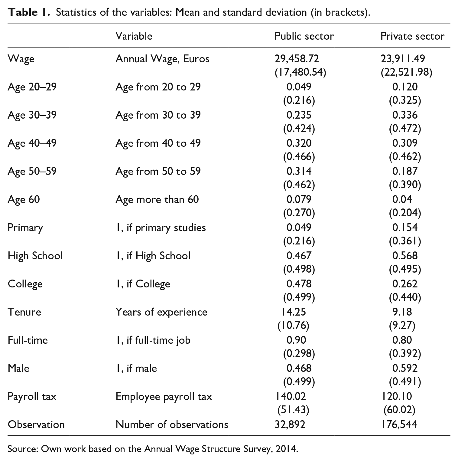
The variables selected for estimating earnings equations are those conventionally used for predicting earnings in labour productivity models: gender, age, level of education, work experience, tenure and full-time job. Earnings, the dependent variable, is measured as usual by annual wage (in logs). The survey considers that there is public control if the public administration owns more than 50% of the stock capital or holds the majority of votes on the board or governing body. The public bodies considered are the central administration, the regional governments and publicly run firms. As a necessary identification constraint in this framework, at least one of the explanatory variables included in the participation equation (probit) must be excluded from the wage equation. This is because the inverse Mills ratio (IMR) is a non-linear function of the explanatory variables in the probit equation; thus, the second stage equation (wage function) is identified because of this non-linearity. The variable considered for identification purpose is payroll taxes. The variables and their means are listed in Table 1.

Table 1.

Statistics of the variables: Mean and standard deviation (in brackets).

	Variable	Public sector	Private sector
Wage	Annual Wage, Euros	29,458.72 (17,480.54)	23,911.49 (22,521.98)
Age 20–29	Age from 20 to 29	0.049 (0.216)	0.120 (0.325)
Age 30–39	Age from 30 to 39	0.235 (0.424)	0.336 (0.472)
Age 40–49	Age from 40 to 49	0.320 (0.466)	0.309 (0.462)
Age 50–59	Age from 50 to 59	0.314 (0.462)	0.187 (0.390)
Age 60	Age more than 60	0.079 (0.270)	0.04 (0.204)
Primary	1, if primary studies	0.049 (0.216)	0.154 (0.361)
High School	1, if High School	0.467 (0.498)	0.568 (0.495)
College	1, if College	0.478 (0.499)	0.262 (0.440)
Tenure	Years of experience	14.25 (10.76)	9.18 (9.27)
Full-time	1, if full-time job	0.90 (0.298)	0.80 (0.392)
Male	1, if male	0.468 (0.499)	0.592 (0.491)
Payroll tax	Employee payroll tax	140.02 (51.43)	120.10 (60.02)
Observation	Number of observations	32,892	176,544

Source: Own work based on the Annual Wage Structure Survey, 2014.

As can be seen, public sector workers in Spain are older: 31.5% are aged between 50 and 59, compared to 18.7% in the private sector. Moreover, in the public sector, the percentage of workers with higher education qualifications is 47.8%, compared to 26.2% in the private sector. The number of women is much higher in the public sector (53.2%) than in the private sector (40.8%), the proportion of full-time contracts is very high in both sectors and, finally, the average job tenure is greater in public than in the private sector by just over 5 years.

Wage gap

The Oaxaca decomposition is the most popular technique for analysing gender wage discrimination. It breaks down the average wage gap between two demographic groups, which usually, but not exclusively, means men and women. The idea is to estimate the earnings functions for each group separately and the results are used to calculate the percentages of the (log) earnings gaps attributable to the explained part (due to different characteristics) and the unexplained part (discrimination). We consider the model

w_{i j} = x_{i}^{T} β_{j} + u_{i j}

(1)

where j = 1 for public and j = 2 for the private one. Blinder (1973) and Oaxaca (1973) propose calculating the wage gap and its causes by subtracting the group 1 income equation from the group 2 income equation, assuming that the difference between the parameters of the equation corresponds to discrimination. Then

{\bar{x}}_{1}^{T} {\hat{β}}_{1} - {\bar{x}}_{2}^{T} {\hat{β}}_{2} = ({\bar{x}}_{1} - {\bar{x}}_{2}) {\hat{β}}_{2} + {\bar{x}}_{1}^{T} ({\hat{β}}_{1} - {\hat{β}}_{2})

(2)

where ${\bar{x}}_{1}, {\bar{x}}_{2}$ are the values of covariates, on average, in each sector. If there is discrimination, that is, $β_{1} - β_{1} \neq 0$ , the discriminant coefficient (Oaxaca, 1973) can be calculated as

D = \frac{\bar{[} {\bar{w}}_{1} / {\bar{w}}_{2}] - \bar{[} {\bar{w}}_{1} / {\bar{w}}_{2}]^{0}}{\bar{[} {\bar{w}}_{1} / {\bar{w}}_{2}]^{0}}

(3)

where

{[\frac{{\bar{{w}}}_{1}}{{\bar{{w}}}_{2}}]}^{0}

is the proportion that would exist if both groups were paid with the same criteria and $\bar{w_{1}}$ and $\bar{w_{2}}$ are the average wages.

Expression 2 has conventionally been used in the standard literature, but it has some important drawbacks: (1) if the selection process is not random and is thus endogenously determined, the Ordinary Least Squares estimates will be biased. However, this problem can be solved by developing some correction terms (control function approach), as the next section proposes; (2) The Oaxaca decomposition only takes into account divergences in the mean, but in general, more information is provided by analysing the whole wage distribution and letting the effects differ at any point within it. Considering this problem, we study the gender wage gap by sectors, including correction terms to solve selection bias and extending the analysis to the whole distribution and not just the mean because there are major discrepancies in the tails of the wage distribution.

Empirical quantile regression literature in economics has become popular recently. The theoretical framework for this estimation is based on the quantilic regression methodology developed by Koenker and Bassett (1978) and applied in the context of wage equations by Chamberlain (1994) and Machado and Mata (2005), among others. Amemiya (1985) was the first to consider quantile regression methods in the presence of endogenous covariates. He shows the consistency and asymptotic normality of two-step median regression estimators. Assume this model

w_{i j} = x_{i}^{T} β_{j}^{θ} + u_{i j}^{θ}

(4)

We assume that the θth quantile of the conditional distribution of the endogenous variable (wages) is a linear function of covariates (worker’s characteristics, xi). Quantile regression is based on minimising weighted absolute deviations to estimate conditional quantile functions, so it can be employed to explain the determinants of the dependent variable at any point of the distribution. Thus, the difference in the (log) wages between the public and private sectors can be written as

Q_{θ} (w_{i 1}) - Q_{θ} (w_{i 2}) = \sum {\hat{β}}_{2}^{θ} ({\bar{x}}_{1} - {\bar{x}}_{2}) + \sum {\bar{x}}_{1} ({\hat{β}}_{1}^{θ} - {\hat{β}}_{2}^{θ})

(5)

Koenker and Bassett (1978) show that quantiles can be estimated by minimising (βθ; βθ). But this approach does not consider sample selection bias. We can, however, combine the decomposition technique with quantile regressions to determine the effects of interest at various points in the wage distribution. We employ the method proposed by Melly (2006) to decompose the gap in a way similar to an Oaxaca–Blinder decomposition but using the complete marginal density distribution.

Econometric methodology

To account for the sample selection problem, we start by considering a structural econometric model of labour supply. The simplest form of this model is the Mincer and Polacheck (1974) human capital earnings equation, which states that the individual (log) wage depends on education, labour market work experience and a random unobservable component. We adapt this model to consider the public and private sectors (see also Arulampalam et al., 2007). Following this approach, the model takes the following form:

w_{i j} = x_{i}^{T} β_{j} + u_{i j} i f f s_{i j}

(6)

where

\begin{array}{l} s_{i j} = 1 (s_{i j}^{*} > 0) = 1 (w_{i j} β_{w} + z_{i}^{T} γ + η_{i j} > 0) \\ = 1 [(x_{i}^{T} β_{j} + u_{i j}) β_{w} + z_{i}^{T} γ + η_{i j} > 0] \\ = 1 (x_{i}^{T} β_{j} β_{w} + z_{i}^{T} γ + β_{w} u_{i j} + η_{i j} > 0) \\ = 1 (x_{i}^{T} α_{j} + z_{i}^{T} γ + v_{i j} > 0) \end{array}

(7)

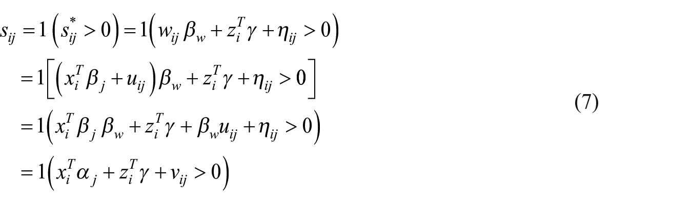
The variable w_ij is the outcome variable of interest: it is the (log) annual wage for the ith individual in sector j (public or private sector); x is a vector of individual characteristics, the variable s_ij is a binary indicator variable set to 1 if person i is in the j sector and 0 otherwise, 1 (A) denotes the indicator function, that is, 1 (A) = 1 if A is true, and 0 otherwise. As usual, the β_j, β_w and γ are parameters to be estimated (we define α_j = (β_jβ_w) and v_ij = (β_wu_ij + η_ij)) and the vector (u_ij, η_ij) is an unobserved idiosyncratic error.

In this context, equation (6) stands for the so-called wage equation, and equation (7) specifies the participation model in each sector j, which depends simultaneously on the wage that an individual expects in the public and other personal characteristics. One of the most important characteristics included in x affecting wages is gender, which is a binary variable that we denote by d.

The first problem is that if the $E [u_{i j} | x_{i}, s_{i j}^{*} > 0]$ is different from 0 in equation (6), then Ordinary Least Squares Estimates are asymptotically biased. The estimation procedure proposed is therefore based on the idea of two-step selection models, with the following switching introduced to the importance of gender in all types of discrepancies concerning wages

If d_{i} = 0, s_{i 1} = 1 : w_{i j} = x_{i}^{T} β_{1}^{0} + u_{i 1}^{0}

(8)

If d_{i} = 0, s_{i 2} = 1 : w_{i j} = x_{i}^{T} β_{2}^{0} + u_{i 2}^{0}

(9)

If d_{i} = 1, s_{i 1} = 1 : w_{i j} = x_{i}^{T} β_{1}^{1} + u_{i 1}^{1}

(10)

If d_{i} = 1, s_{i 2} = 1 : w_{i j} = x_{i}^{T} β_{2}^{1} + u_{i 2}^{1} i = 1, \dots, N

(11)

And then

E (w_{i j} | x_{i}, d_{i} = 0, s_{i 1} = 1) = x_{i}^{T} β_{1}^{0} + E (u_{i 1}^{0} | d_{i} = 0, s_{i 1} = 1)

(12)

E (w_{i j} | x_{i}, d_{i} = 0, s_{i 2} = 1) = x_{i}^{T} β_{2}^{0} + E (u_{i 2}^{0} | d_{i} = 0, s_{i 2} = 1)

(13)

E (w_{i j} | x_{i}, d_{i} = 1, s_{i 1} = 1) = x_{i}^{T} β_{1}^{1} + E (u_{i 1}^{1} | d_{i} = 1, s_{i 1} = 1)

(14)

E (w_{i j} | x_{i}, d_{i} = 1, s_{i 2} = 1) = x_{i}^{T} β_{2}^{1} + E (u_{i 2}^{1} | d_{i} = 1, s_{i 2} = 1)

(15)

If there is evidence of non-normal disturbances in the reduced equation, then it is not correct to estimate the participation decision by Probit Maximum Likelihood and in that case, the so-called IMR is misspecified. In such cases, a partially linear model could be estimated using a non-parametric function instead of standard IMR using the approach suggested by Arellano and Bonhomme (2017).

On the contrary, if the participation error (v_ij) is distributed as a standardised normal, the probit maximum likelihood estimators of the first stage are consistent and the Mills ratio is thus a suitable way to correct for the bias. The procedure proposed for estimating the structural parameters of this model is as follows:

Step 1: The reduced participation equation, equation (6), is estimated by Probit Maximum Likelihood.

Step 2: With the parameters estimated from the first step, the modified IMR terms required to approximate the unknown correction terms and estimate the wage equation to obtain consistent estimates can be estimated (equations (11)–(14)).

Step 3: Finally, to estimate the effects in the structural equation, a decomposition of the wage gaps applied to both the standard regression model and Quantile Regression estimates is presented.

In line with the seminal papers in the field, we use the standard methodology for analysing sector wage gaps. Melly (2006) proposes an intuitive procedure for decomposing differences at different quantiles of the unconditional distribution and shows that this estimator is consistent and asymptotically normally distributed. Consistent estimators of variances are also proposed. Accordingly, the cdeco STATA command is used to estimate the conditional quantiles at each percentile of the test score distribution (Chernozhukov et al., 2013). Bootstrapped standard errors are bootstrapped using 100 replications, using the asymptotic properties by Chernozhukov et al. (2013).

Results

Summary statistics

As can be seen in Table 1, the difference in average annual wages between the two sectors is just over 5500 Euros in favour of the public sector. Moreover, almost half of the workers in the public sector have higher education qualifications (25% in the private sector), average job tenure is almost 5 years longer in the public and approximately 47% of public sector workers are men, compared to 59.2% of private sector workers.

Figure 1 shows the distribution of annual (log) wages. The (log) wages in the public sector have a higher mean and a lower standard deviation than those in the private sector. Moreover, the tails of this distribution are substantially larger in the private sector, that is, there are workers with much lower and higher wages, on average, in the private sector. Therefore, it seems reasonable to think that the sector where an individual works is a determining factor for the wages received.

Figure 1.

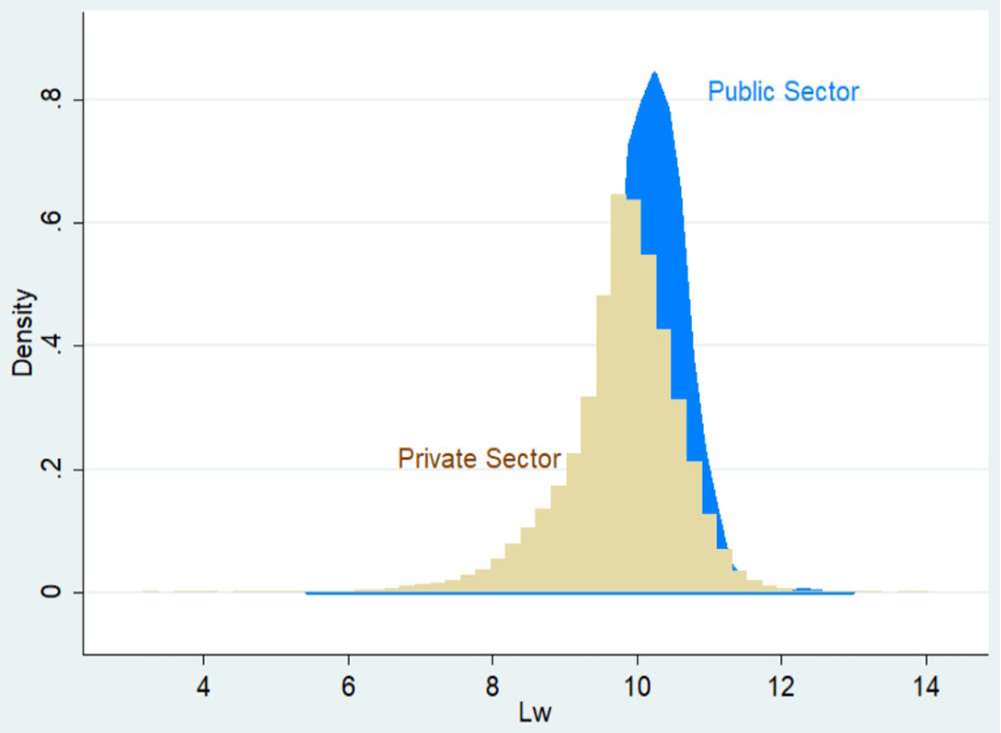
Density function by sector.

In the first graph in Figure 2, the left tail is longer for women, which reveals that in the public sector, women have lower wages than men; the second graph in Figure 2 shows that the average wage is higher in the public sector than in the private one for both men and women.

Figure 2.

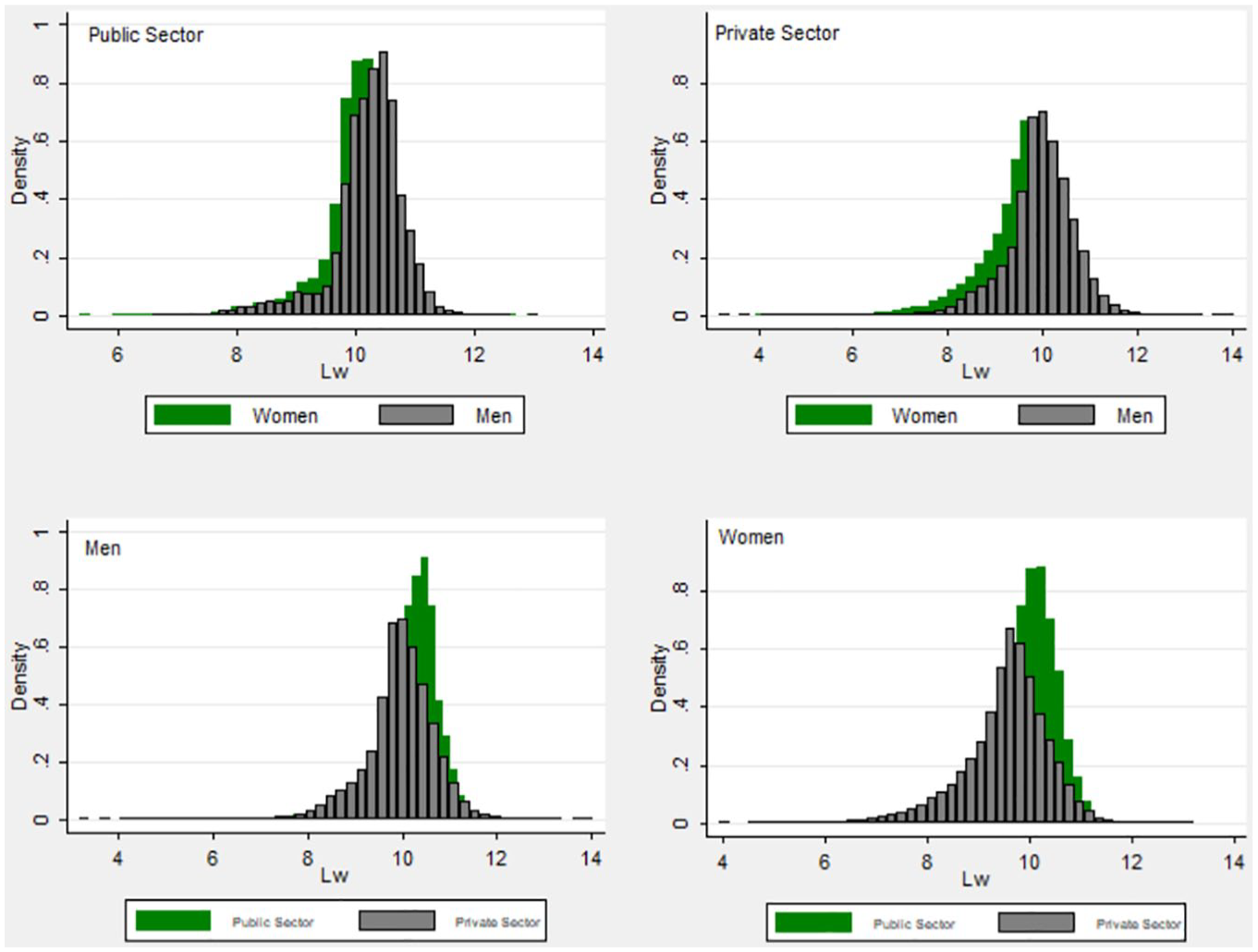
Wage density by sector.

Taking into account that the dependent variable is used in logarithm form, there is no reason to suspect non-normality in the structural equation based on the above graphs. Thus, the IMR can be used to approximate the correction terms.

Estimation results

To estimate the gender wage gap, we first distinguish between the explained part (differences in endowments or characteristics) and the unexplained part (discrimination) in the two sectors. We then compare the components of the wage gap over the quantiles and across sectors. Estimates are calculated with STATA statistical software. Table 7 in Appendix 1 shows the results of equation (5) using a standard Ordinary Least Squares estimation for each sector with no correction. As argued throughout the article, this is used merely to give an initial intuition of the effects, because they will be inconsistent.

In the first step of the estimation procedure proposed, we regress the binary selection variable (public/private job) on some explanatory variables as proposed in equation (6) by calculating a probit model, thus obtaining the IMR (Table 8 in Appendix 1). As can be seen in Table 8 in Appendix 1, the probability of working in the public sector increases with education (as expected due to the entry process), decreases with age and is lower for men. Once again, all the variables are statistically significant.

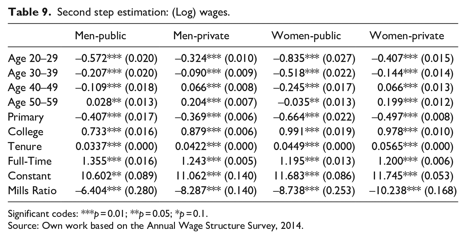
As pointed out in the previous section, it is possible to re-estimate equation (5) by including the necessary sample selection correction term in each case. These results are presented in Table 9 in Appendix 1, desegregating the four possible cases (di = 1, si1 = 1), (di = 1, si2 = 1), (di = 0, si1 = 1) and (di = 0, si2 = 1) developed in equations (7) to (10). In most cases, age, education, experience and full-time work are factors expected to increase wages. It is interesting to highlight that the effects of further education are similar for men and women in the public sector, but its effect is considerably higher for men in the private sector. Working full-time has a higher effect on wages for men than for women in both sectors. The private sector also pays much more for further education qualifications than the public sector for men, but not for women. Finally, there is a statistically significant self-selection term in all four groups considered (Table 9 in Appendix 1).

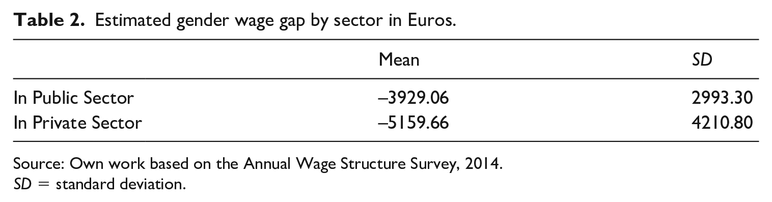
Table 2 shows the gender wage gap estimated in the two sectors once the model proposed is estimated. It can be seen that in the private sector, men earn 5159 Euros more than women but in the public sector, the figure is only 3929. That is, gender pay discrimination is estimated to average around 14% in the public and around 19.9% in the private sector. Moreover, there is more dispersion in the private sector.

Table 2.

Estimated gender wage gap by sector in Euros.

	Mean	SD
In Public Sector	–3929.06	2993.30
In Private Sector	–5159.66	4210.80

Source: Own work based on the Annual Wage Structure Survey, 2014.

SD = standard deviation.

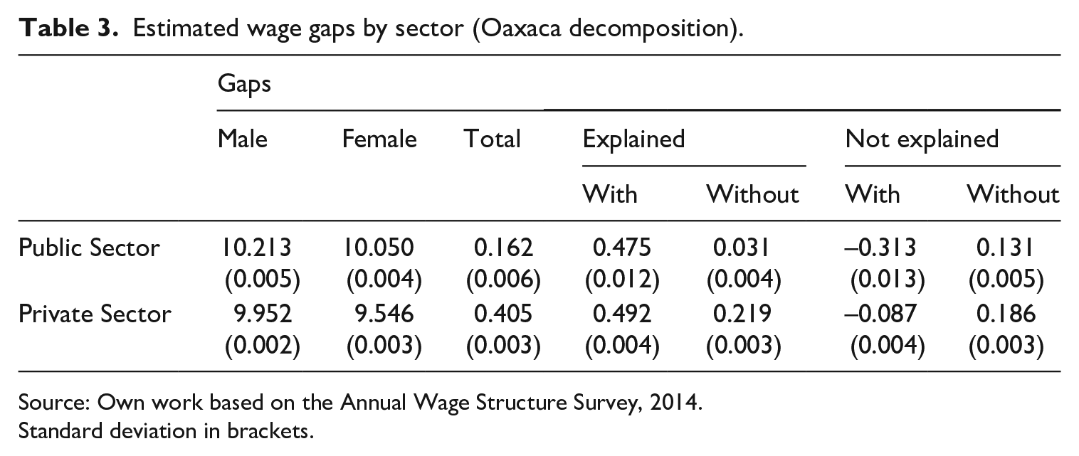
Next, we analyse the causes of the differences by decomposing the different effects (Table 3).

Table 3.

Estimated wage gaps by sector (Oaxaca decomposition).

	Gaps
	Male	Female	Total	Explained		Not explained
	Male	Female	Total	With	Without	With	Without
Public Sector	10.213 (0.005)	10.050 (0.004)	0.162 (0.006)	0.475 (0.012)	0.031 (0.004)	–0.313 (0.013)	0.131 (0.005)
Private Sector	9.952 (0.002)	9.546 (0.003)	0.405 (0.003)	0.492 (0.004)	0.219 (0.003)	–0.087 (0.004)	0.186 (0.003)

Source: Own work based on the Annual Wage Structure Survey, 2014.

Standard deviation in brackets.

The Oaxaca decomposition (Table 3) shows the mean predictions by sectors and gender and the differences between them. Both the gaps explained by endowments and the unexplained gaps (discrimination) are also corrected for endogeneity. In our sample, the geometric mean of wages in the public sector is around 27,269 Euros for men and 23,177 for women, giving a gap of about 16.2%. This means that in the public sector, men’s wages are on average about 16% higher than those of women. Adjusting women’s endowment levels in regard to those of men increases women’s wages by 3.1% but a gap of 13.1% remains unexplained. If a term is included to correct for the endogenous choice of sector, the effect due to differences in characteristics increases women’s wages by 47.5% but a gap of 31.3% remains unexplained.¹

The mean wage for women is round 13,999 Euros in the private sector compared to about 21,001 for men, so wages in the private sector are about 40.5% higher for men than for women. Adjusting men’s endowment levels in regard to those of women increases women’s wages by 21.8%. A gap of 18.6% remains unexplained. If the correction term is introduced, the results change, and adjusting men’s endowment levels to those of women increases women’s wages by 49.2%. A gap of 8.7% remains unexplained. Next, the complete distribution of wages is analysed using quantile regression and the correction method proposed in this article.

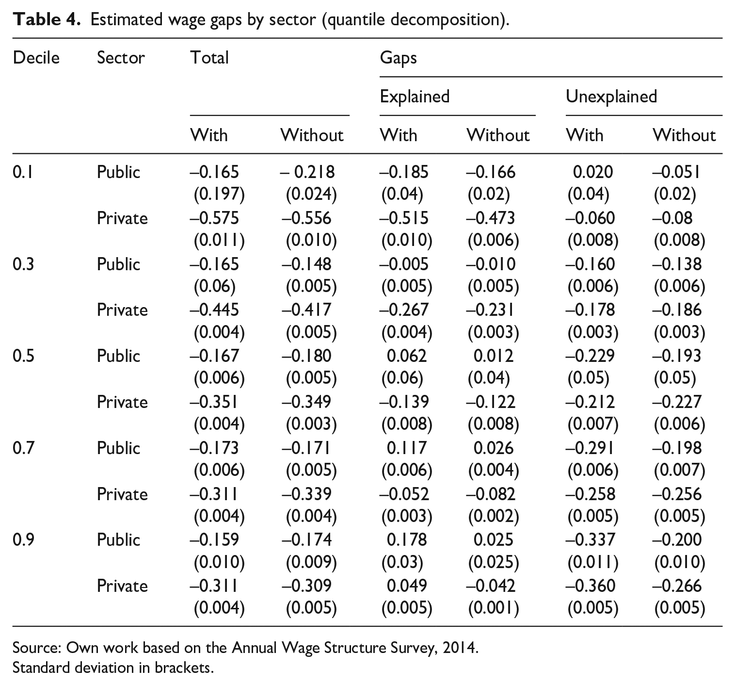
Table 4 shows the gender gaps (women–men) by sectors. As can be seen, in both sectors, there is a negative wage gap for women throughout the wage distributions. The biggest difference between the observable distributions is 17.3% in the 70th quantile, while the smallest is at the top end of the distribution, in the 90th quantile. It can also be observed that the gap is wider in the private sector for all points of the distribution, at 57.5% in the 10th and decreasing as one moves up the wage distribution.

Table 4.

Estimated wage gaps by sector (quantile decomposition).

Decile	Sector	Total		Gaps
		Total		Explained		Unexplained
		With	Without	With	Without	With	Without
0.1	Public	–0.165 (0.197)	– 0.218 (0.024)	–0.185 (0.04)	–0.166 (0.02)	0.020 (0.04)	–0.051 (0.02)
0.1	Private	–0.575 (0.011)	–0.556 (0.010)	–0.515 (0.010)	–0.473 (0.006)	–0.060 (0.008)	–0.08 (0.008)
0.3	Public	–0.165 (0.06)	–0.148 (0.005)	–0.005 (0.005)	–0.010 (0.005)	–0.160 (0.006)	–0.138 (0.006)
0.3	Private	–0.445 (0.004)	–0.417 (0.005)	–0.267 (0.004)	–0.231 (0.003)	–0.178 (0.003)	–0.186 (0.003)
0.5	Public	–0.167 (0.006)	–0.180 (0.005)	0.062 (0.06)	0.012 (0.04)	–0.229 (0.05)	–0.193 (0.05)
0.5	Private	–0.351 (0.004)	–0.349 (0.003)	–0.139 (0.008)	–0.122 (0.008)	–0.212 (0.007)	–0.227 (0.006)
0.7	Public	–0.173 (0.006)	–0.171 (0.005)	0.117 (0.006)	0.026 (0.004)	–0.291 (0.006)	–0.198 (0.007)
0.7	Private	–0.311 (0.004)	–0.339 (0.004)	–0.052 (0.003)	–0.082 (0.002)	–0.258 (0.005)	–0.256 (0.005)
0.9	Public	–0.159 (0.010)	–0.174 (0.009)	0.178 (0.03)	0.025 (0.025)	–0.337 (0.011)	–0.200 (0.010)
0.9	Private	–0.311 (0.004)	–0.309 (0.005)	0.049 (0.005)	–0.042 (0.001)	–0.360 (0.005)	–0.266 (0.005)

Source: Own work based on the Annual Wage Structure Survey, 2014.

Standard deviation in brackets.

As can be seen, in the public sector, the effect of characteristics (explained differences) against women is declining at the top of the wage distribution. At this end of the distribution, it can be observed that gaps are attributable more to the coefficients effect (unexplained differences). In the private sector, the pattern is similar but stronger, with wider gaps (see also Figure 3).

Figure 3.

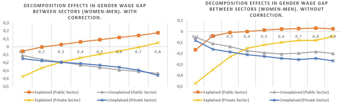
Estimated gender wage gap between sectors.

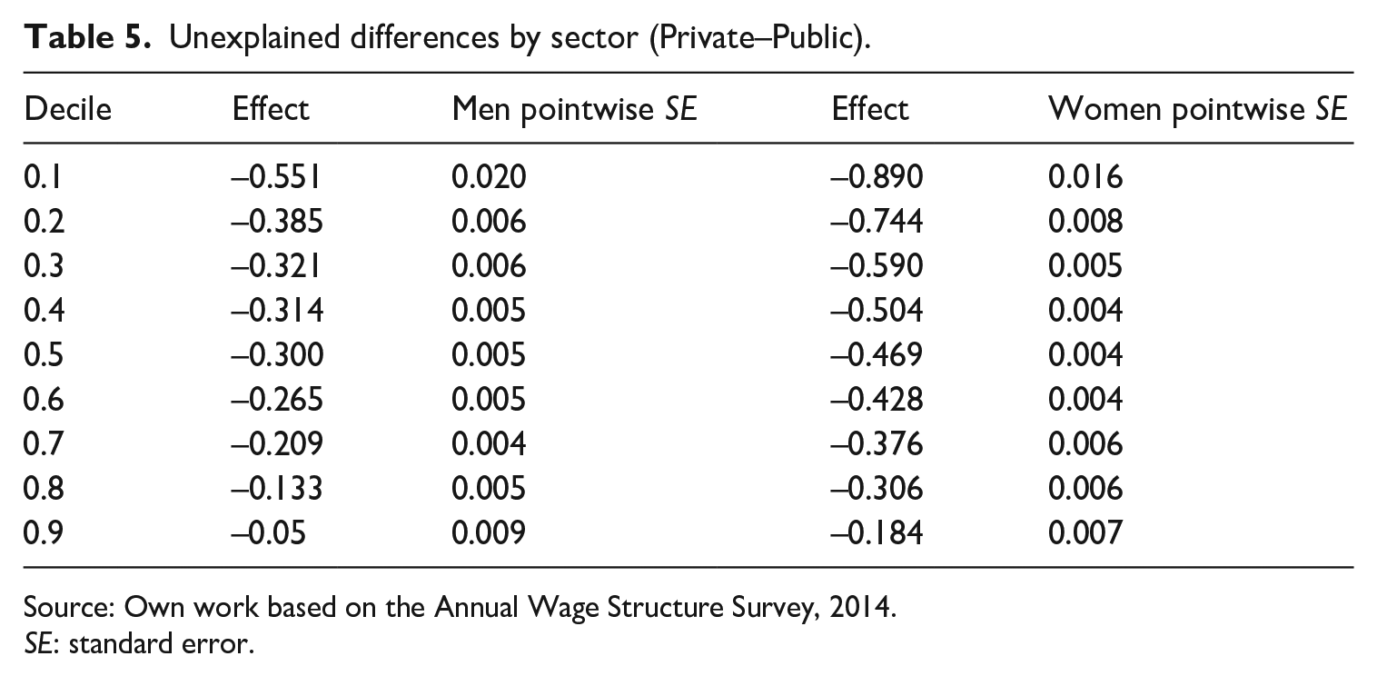
Table 5 shows that the first decile of the private sector wage distribution is around 55% lower than the first decile of the public sector wage distribution. At the median, it is 30% lower. Note that these gaps narrow at the top end of the wage distribution. For women, the pattern throughout the distribution is similar to that for men but with higher figures. At the median, the private sector wage distribution is 46.9% lower than that of the public sector.

Table 5.

Unexplained differences by sector (Private–Public).

Decile	Effect	Men pointwise SE	Effect	Women pointwise SE
0.1	–0.551	0.020	–0.890	0.016
0.2	–0.385	0.006	–0.744	0.008
0.3	–0.321	0.006	–0.590	0.005
0.4	–0.314	0.005	–0.504	0.004
0.5	–0.300	0.005	–0.469	0.004
0.6	–0.265	0.005	–0.428	0.004
0.7	–0.209	0.004	–0.376	0.006
0.8	–0.133	0.005	–0.306	0.006
0.9	–0.05	0.009	–0.184	0.007

Source: Own work based on the Annual Wage Structure Survey, 2014.

SE: standard error.

The estimated unexplained wage gap (coefficient effect) varies depending on which quantile is chosen. For men, it varies from 20% in θ = 0.1 to 16% in θ = 0.9. For women, it varies from −15% in θ = 0.1 to 21.6% in θ = 0.9. By contrast, the characteristics gap seems to be more stable across the distribution, though for men, there is more variation with θ than for women. The unexplained part of the sector wage gap is decreasing across the wage distribution up to the median for women and up to quantile 0.6 for men. Finally, accounting also for the characteristics effect, our results show that, as expected, the wage gap for public employees is especially wide for low-income earners. At the upper end of the wage distribution, the gap is narrower (see Figure 4).

Figure 4.

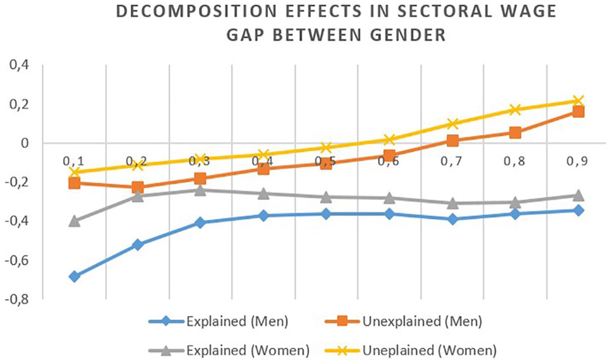
Estimated gaps between sectors.

Our results show that both the gender wage gap as a whole and the unexplained gap are larger in the private sector than in the public one. Moreover, the reduction in the gross gender wage gap is greater in the private sector than in the public sector (one-half compared with one-quarter).

Conclusion

In this article, we investigate the public–private sector gender wage gap using Spanish microdata, seeking to provide new evidence on the gender wage gap between these sectors in Spain. To that end, we propose a model that corrects for the selectivity bias of the sample, considering the prior process of choosing the sector and additionally switching it by gender. Our findings suggest that there is discrimination against women in both the public and private sectors, but less so in the former. Women are paid less than men, even when the distribution of characteristics is kept constant in the analysis. This result is consistent with the findings of recent reviews for Spain and other countries: Hospido and Moral Benito (2016) and De La Rica et al. (2015) for Spain, Cai and Liu (2011) for Australia and Bargain et al. (2018) for France. The size of the gaps attributed to different returns varies substantially across the distribution of wages (Antón and Muñoz de Bustillo, 2015).

However, the gender wage gap between the public and private sectors decreases as one moves up the wage distribution. In general, wage gap estimates suggest that individuals are better off working in the public sector, especially in the lowest deciles. The opposite is true for men in the highest deciles. The evidence seems to indicate that there is a glass-ceiling effect in private sector pay for women (in the top deciles) and a sticky floor effect for the private sector pay of low-skilled women (De La Rica et al., 2015; Hospido and Moral Benito, 2016).

It can also be observed that the conditional distribution of wages in the public sector is more compressed than the wage distribution in the private sector, that is, the wage distribution has a lower standard deviation in the public sector. We suggest that the endogenous selection problem is likely to contribute to these differences. Including correction terms in the estimation suggests that taking into account the selection mechanism increases the size of the gap due to characteristics and reduces the unexplained part. An examination of the whole wage distribution reveals that the gaps are in general somewhat smaller with the corrections than without them, but are still very similar. On the contrary, the explained part of the gaps is larger when the correction is used. For the sector wage gap, the unexplained wage gap (coefficient effect) estimated varies with the chosen quantile and the characteristics gap seems to be more stable. Moreover, the unexplained part is decreasing across the wage distribution up to the median for women (and up to quantile 0.6 for men).

These results have important policy implications: first, empirical evidence confirms that the public sector is a fair employer, as it has both a lower gender wage gap and a more compressed pay dispersion than the private sector (Cai and Liu, 2011), but governments should consider how to continue to reduce gender wage gaps in the public sector. Moreover, the existence of a positive public–private wage gap across most of the wage distribution also means that the public sector pays more than the opportunity wage for low-skilled labour but less than what is needed to attract, retain and motivate high-skilled workers (Bargain et al., 2018). Second, the differences in the private sector are highly significant, so policy-makers need to propose measures to achieve equal pay in private companies. In this regard, gender equality policies have been implemented recently, such as legislation in Spain promoting workplace equality between men and women through compulsory implementation of a workplace equality plan at companies with 50 or more employees (previously 250 or more employees) and increasing paternity leave to 16 weeks by 2021. In the European Union, gender equality policies are becoming a priority and governments are working to reduce current differences. Elomäki (2015) declares that the absence of feminist voices from the initial shaping of the policy problem is seen as an important factor behind the economisation of the debate on gender equality and decision-making at European Union level, with the issue of business leadership taking priority (p. 13).

As regards future research, we believe that a multi-level hierarchical model could help group workers by occupations and then by sectors, to address questions such as whether graduates working in education or health earn, on average, more (or less) than non-graduates engaged in manufacturing activities.

Footnotes

Appendix 1

Table 9.

Second step estimation: (Log) wages.

	Men-public	Men-private	Women-public	Women-private
Age 20–29	–0.572*** (0.020)	–0.324*** (0.010)	–0.835*** (0.027)	–0.407*** (0.015)
Age 30–39	–0.207*** (0.020)	–0.090*** (0.009)	–0.518*** (0.022)	–0.144*** (0.014)
Age 40–49	–0.109*** (0.018)	0.066*** (0.008)	–0.245*** (0.017)	0.066*** (0.013)
Age 50–59	0.028** (0.013)	0.204*** (0.007)	–0.035** (0.013)	0.199*** (0.012)
Primary	–0.407*** (0.017)	–0.369*** (0.006)	–0.664*** (0.022)	–0.497*** (0.008)
College	0.733*** (0.016)	0.879*** (0.006)	0.991*** (0.019)	0.978*** (0.010)
Tenure	0.0337*** (0.000)	0.0422*** (0.000)	0.0449*** (0.000)	0.0565*** (0.000)
Full-Time	1.355*** (0.016)	1.243*** (0.005)	1.195*** (0.013)	1.200*** (0.006)
Constant	10.602** (0.089)	11.062*** (0.140)	11.683*** (0.086)	11.745*** (0.053)
Mills Ratio	–6.404*** (0.280)	–8.287*** (0.140)	–8.738*** (0.253)	–10.238*** (0.168)

Significant codes: ***p = 0.01; **p = 0.05; *p = 0.1.

Source: Own work based on the Annual Wage Structure Survey, 2014.

Declaration of Conflicting Interests

The author(s) declared no potential conflicts of interest with respect to the research, authorship and/or publication of this article.

Funding

The author(s) disclosed receipt of the following financial support for the research, authorship and/or publication of this article: The authors acknowledge financial support from the Programa Estatal de Fomento de la Investigacion Cientifica y Técnica y de Innovación / Spanish Ministry of Economy and Innovation. Ref: P ID2019 − 105986GB − C22.

ORCID iD

Patricia Moreno-Mencía

Notes

References

Alaez

Ullibarri

(2001) Diferencias salariales entre los sectores pu’blico y privado por género, escolaridad y edad. El caso de España. ICE. Tribuna de Econom’ıa 789: 117–138.

Amemiya

(1985) Advanced Econometrics. Cambridge, MA: Harvard University Press.

Antón

Muñoz

Bustillo

(2015) Public-private sector wage differentials in Spain. An updated picture in the midst of the Great Recession. Investigacio’n Econ’omica 74(292): 115–157.

Arellano

Bonhomme

(2017) Quantile selection models with an application to understanding changes in wage inequality. Econometrica 85: 1–28.

Arulampalam

Booth

Bryan

(2007) Is there a glass ceiling over Europe? Exploring the gender pay gap across the wage. ILR Review 60: 163–186.

Bargain

Etienne

Melly

(2018) Public sector wage gaps over the long-run: Evidence from panel administrative data. Discussion paper 119 24, October. Bonn: IZA.

Becker

(1964) Human Capital. New York: Columbia University Press.

Belgorodskiy

Crump

Griffiths

, et al. (2012) The gender pay gap in the ICT labour market: Comparative experiences from the UK and New Zealand. New Technology Work and Employment - NEW TECHNOL WORK EMPLOY 27(2). DOI: 10.1111/j.1468-005X.2012.00281.x

Blau

Kahn

(2007) Changes in the labor supply behavior of married women: 1980-2000. Journal of Labor Economics 25: 393–438.

10.

Blinder

(1973) Wage discrimination: Reduced form and structural variables. The Journal of Human Resources 8: 436–455.

11.

Cai

Liu

(2011) Public–private sector wage gap in Australia: Variation along the distribution. British Journal of Industrial Relations 49(2): 362–390.

12.

Chamberlain

(1994) Quantile regression, censoring, and the structure of wages. In: Sims

(ed.) Advances in Econometrics: Sixth World Congress (Econometric Society Monograph). New York: Cambridge University, pp. 171–209.

13.

Chernozhukov

Fernandez

Melly

(2013) Inference on counterfactual distributions. Econometrica 81: 2205–2268.

14.

De La Rica

Dolado

Vegas

(2015) Gender gaps in performance pay: New evidence from Spain. Annals of Economics and Statistics, GENES 117: 41–59.

15.

Elomäki

(2015) The economic case for gender equality in the European Union: Selling gender equality to decision-makers and neoliberalism to women’s organizations. European Journal of Women’s Studies 22(3): 288–302.

16.

European Commission (2015) Women in the labour market. European Commission. Available at: https://ec.europa.eu/info/sites/info/files/european-semester_thematic-factsheet_labour-force-participation-women_en_0.pdf

17.

European Commission (2018) The gender pay gap situation in the EU. Available at: https://ec.europa.eu/info/policies/justice-and-fundamental-rights/gender-equality/equal-pay/gender-pay-gap-situation-eu_en

18.

Fitzsimons

(2017) Gender as a Verb: Gender Segregation at Work. London: Routledge.

19.

Grimshaw

Fagan

Hebson

, et al. (2017) Making Work More Equal. A New Labor Market Segmentation Approach. Manchester: Manchester University Press.

20.

Hospido

Moral Benito

(2016) The public sector wage premium in Spain: Evidence from longitudinal administrative data. Labor Economics 42: 101–122.

21.

Jann

(2005) Standard errors for the Blinder-Oaxaca decomposition. 3rd German Stata Users Group Meeting, Berlin, 8 April.

22.

Koenker

Bassett

(1978) Regression quantiles. Econometrica 46: 33–50.

23.

Kreimer

(2004) Labour market segregation and the gender-based division of labour. European Journal of Women’s Studies 11(2): 223–246.

24.

Machado

Mata

(2005) Counterfactual decomposition of changes in wage distributions using quantile regression. Journal of Applied Econometrics 20: 445–465.

25.

Mandel

(2013) Up the down staircase: Women’s upward mobility and the wage penalty for occupational feminization, 1970-2007. Social Forces 91: 1183–1207.

26.

Mandel

Semyonov

(2014) Gender pay gap and employment sector: Sources of earnings disparities in the U.S., 1970-2010. Demography 51: 1597–1618.

27.

Melly

(2006) Estimation of counterfactual distributions using quantile regression. Discussion Paper, University of St. Gallen.

28.

Mincer

Polacheck

(1974) Family investments in human capital: Earnings of women. Journal of Political Economy 82(5): 76–108.

29.

Oaxaca

(1973) Male-female wage differentials in urban labor markets. International Economic Review 14: 693–709.

30.

Organisation for Economic Co-operation and Development (OECD) (2019) Gender Equality in Politics in Government at a Glance. Paris: OECD.

31.

Petersen

Morgan

(1995) Separate and unequal: Occupation establishment segregation and the gender wage gap. American Journal of Sociology 101: 329–365.

32.

Rubery

Grimshaw

Figueiro

(2005) How to close the gender pay gap in Europe: Towards the gender mainstreaming of pay policy. Industrial Relations Journal 36(3): 184–213.

33.

Segovia-Perez

Castro-Nuñez

Santero-Sanchez

, et al. (2020) Ser mujer en un trabajo de TIC: un análisis de la brecha salarial de género y la discriminación en España. Nuevas tecnologías, trabajo y empleo 35(1): 20–39.

34.

Spanish National Securities Market Commission (CNMV) (2019) Data on the presence of women on the boards of directors and in the senior management positions of each of the listed companies. Available at: http://cnmv.es/portal/Publicaciones/Consejeras_Directivas.aspx?lang=en

35.

Suh

(2017) Determinants of female labor force participation in South Korea: Tracing out the u-shaped curve by economic growth. Social Indicators Research 131(1): 255–269.

36.

Treiman

Hartmann

(1981) Women, Work and Wages: Equal Pay for Jobs of Equal Value. Washington, DC: National Academy Press.

37.

Weeden

(2004) Profiles of change: Sex segregation in the United States, 1910-2000. In: Charles

Grusky

(eds) Occupational Ghettos: The Worldwide Segregation of Women and Men. Palo Alto, CA: Stanford University, pp. 131–178.

38.

World Economic Forum (2020) Global Gender Gap Report. Geneva: World Economic Forum.