Electoral coordination and party system institutionalization

Abstract

A new theoretical development for examining the institutionalization of party systems is proposed in this article. We build on electoral coordination theories to disaggregate volatility into the vote transfers that occur between or towards parties that are in equilibrium (which we call endogenous volatility) and those that are not (exogenous volatility). The former captures accountability, and the latter reflects the number of voters who are not acting in accordance with the existing equilibrium in the party system. Exogenous volatility measures the institutionalization of party systems. We also show that endogenous volatility depends on government performance, while exogenous volatility is a function of institutional openness. The empirical evidence comes from an original data set that includes 448 electoral cycles in lower-house elections in 66 countries between 1977 and 2011.

Keywords

accountability coordination equilibrium party system institutionalization volatility

The transitions to democracy in Latin America, Asia and Eastern Europe and the resurgent multi-partism in Africa in recent decades have been accompanied by increasing attention to party system institutionalization in comparative politics. The institutionalization of party systems refers to the situation in which ‘actors develop expectations and behaviour based on the premise that the fundamental rules of party competition and behaviour will prevail into the foreseeable future’ (Mainwaring and Torcal, 2006: 206) and captures ‘the degree to which competitive political regimes develop stable patterns of interparty competition’ (Mainwaring and Zoco, 2007: 156). The stability of interparty competition, the first and most basic dimension of party system institutionalization (Mainwaring and Scully, 1995), is conventionally measured with the Pedersen volatility index (Pedersen, 1979, 1983), a comprehensive measure of the net systematic shift in the levels of party electoral support across elections. As volatility is negatively correlated with party system institutionalization, the conventional wisdom holds that political representation deteriorates when there is persistent high volatility.

Recently, Tavits (2008), Sanchez (2009), Powell and Tucker (2014), Weghorst and Bernard (2014), Chiaramonte and Emanuele (2017) and Mainwaring et al. (2017) have revisited the foundations of the Pedersen index. Their argument is that electoral volatility should be broken down into the volatility that occurs when voters switch their votes between existing (or established) parties and the volatility caused by the entry and exit of parties in the system.

Although these contributions are very valuable, this area of research faces three crucial shortcomings. First, as a consequence of not having clear theoretical foundations, the approach is empiricist. This is reflected in a variety of arbitrary decisions concerning the measurement of the two types of volatility, affecting the estimation and levels of electoral volatility across countries and elections (Casal-Bertoa et al., 2017). Second, there are no clear expectations about the cross-country and cross-temporal determinants of the two types of volatility. Third, not surprisingly, the empirical evidence about the causes of vote transfers between new and established parties is inconclusive. For instance, when re-examining Powell and Tucker’s (2014) analysis of the party system in post-communist countries, Crabtree and Golder (2017) found that none of the variables proposed by Powell and Tucker significantly affects volatility.

In this article, we revisit the theoretical foundations of volatility as a measure of patterns of party system competition which, we argue, achieves an equilibrium when the voters’ demand for parties is reduced to an actual supply of parties through the maximum ‘carrying capacity’ of electoral systems (Cox, 1997).

We make three contributions. The first is conceptual or theoretical. We build on electoral coordination theories to disaggregate volatility into the vote transfers that occur between or towards parties that are in equilibrium (which we call endogenous volatility) and those that are not (exogenous volatility). Equilibria in party systems are not equally stable, as the transaction costs for an alternative electoral coordination differ across countries and districts and over time. To determine whether an equilibrium is perdurable, the crucial piece of information is the exogenous volatility. The lower the exogenous volatility, the greater the institutionalization of the party system. On the other hand, endogenous volatility captures accountability. The greater the endogenous volatility, the more accountable the incumbents.

Our second contribution is explanatory. We show that the cross-country and cross-temporal determinants of endogenous and exogenous volatilities are different. While exogenous volatility is a function of institutional openness, endogenous volatility depends on economic performance.

Finally, our third contribution is empirical. Non-arbitrary empirical rules to measure institutionalization at the district and national levels are provided. The empirical evidence comes from an original data set that includes 448 electoral cycles in lower-house elections in 66 countries between 1977 and 2011.

Arguments

The measurement of party system institutionalization remains an open discussion in comparative politics. The most recent indicators have been proposed by Powell and Tucker (2014), Chiaramonte and Emanuele (2017) and Mainwaring et al. (2017). Powell and Tucker distinguished between volatility caused by new party entry and old party exit (type A volatility or replacement volatility), and volatility caused by vote switching across existing parties (type B volatility or simply electoral volatility). A 2% threshold of the national vote is employed to define whether a party has entered or exited the political system. Chiaramonte and Emanuele also used type A volatility (or volatility by regeneration in their own words) to capture deinstitutionalization. The main difference from the Powell and Tucker model is that they reduced the threshold from 2% to 1% of the national vote when distinguishing between existing and new parties. Mainwaring et al. (2017) built on Powell and Tucker’s type A volatility but referred to it as extra-system volatility. In contrast to Powell and Tucker and Chiaramonte and Emanuele, new parties are not defined in terms of electoral support but according to whether they are competing for the first time or not.

The theoretical foundations of these measures, however, are not clear, and as a result, flawed empirical decisions are made when defining and measuring volatility. First, arbitrary and ad hoc decisions based on party vote shares or party age are the rule. As the effective threshold to gain seats differs greatly across electoral systems (and even across districts within electoral systems), using party support thresholds to determine whether parties are relevant actors in elections is problematic. For instance, in the 2012 and 2017 Dutch national elections, 50PLUS gained two and four seats with 1.9% and 3.1% of the votes, respectively. The same support in a country using a first-past-the-post system would be negligible. Similarly, whether a non-viable party is entering the race for the first or the second time does not make any difference for the stability of the party system; the transaction costs for an alternative coordination are the same.

Second, when using a threshold of the national vote to decide whether a party is new or not, or whether it has left the system or not, the assumption is that each district within an electoral system has the same parties competing with equal strength. However, as the literature on the nationalization of parties and party systems shows (Chhibber and Kollman, 2004), in those countries in which there is a relevant ethnolinguistic cleavage (e.g. Spain or Canada), not all strong and viable local parties attain 1% or 2% of the votes nationally.

Finally, it is crucial to use an idiosyncratic but non-arbitrary rule to count parties as new or existing. Clearly, conceptions of party support do not travel well across countries, districts and elections.

Not surprisingly, when critically examining the state of the art, largely based on the use of the previous measures, Crabtree and Golder (2017: 234) concluded that ‘we know little about what causes party system volatility’.

Party system institutionalization is the result of an equilibrium generated by the strategic behaviour of party elites and voters conditioned by the existing institutions (Sanchez, 2009). Our point of departure is the received wisdom within party politics and electoral studies that a competitive party system is a necessary ingredient of democratic politics only when both the party system and the individual parties are in equilibrium. According to Aldrich (2011: 25),

an individual party is in equilibrium when its label conveys meaning to voters…, and it is sufficiently attractive to enough voters so as, in turn, to attract ambitious politicians to affiliate with it and its label…In a two-party system, then, each of the parties is in equilibrium when elections are competitive. The important point is that each and every incumbent fears losing the next election, and indeed they should because the opposition has a credible chance of winning.

As effective democracy relies on durable parties in strategic interaction, which are expected to continue to be so in the future, we argue that volatility between a pair of elections should be split into (a) that which occurs when votes are switched to parties that are in equilibrium in the first election and (b) that caused by the transfer of votes to parties that are not in equilibrium in the first election. We call the first type endogenous volatility and the second exogenous volatility.

The two types of volatility have opposite consequences for representative democracies. Endogenous volatility is a positive component of representative democracies, because it makes incumbents accountable. According to the traditional interpretation of retrospective voting as a reward–punishment model, voters favour the government when the economy improves and turn against it when the economy deteriorates (Key, 1964: 568). If endogenous volatility is high, it means that voters are rewarding or punishing the incumbent for its performance; however, if exogenous volatility is low both when the economy is doing well or badly, it means that citizens are not abandoning their party in order to reward or punish the incumbent based on performance. In other words, they are rendered blind to economic performance and, therefore, the government is not held accountable. In a recent piece, Schleiter and Voznay (2016: 336) empirically show that it is through stable patterns of party competition and the organizational stability of parties that elections turn into effective mechanisms for voters to align the interests of their representatives with their own and to reduce the scope for governmental corruption. The percentage points of endogenous volatility measure the accountability dimension of volatility.

Exogenous volatility captures the transaction costs for an alternative electoral coordination. The percentage points of exogenous volatility measure the institutionalization of party systems; the lower the exogenous volatility, the greater the institutionalization or the more stable the equilibrium. Of course, we are not saying that party systems have to be rendered blind to emerging demands channelled through new parties. The problem for party systems is when new successful parties repeatedly emerge. When having a longitudinal perspective, the occasional emergence of a new and viable party or even few new and viable parties do not significantly increase exogenous volatility as they are considered viable parties in the second and subsequent elections.

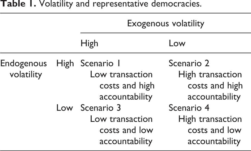
As can be seen in Table 1, the ideal scenario for representative democracies is the combination of low exogenous volatility (i.e. high transaction costs for a new equilibrium) and high endogenous volatility to make incumbents accountable (scenario 2). In contrast, when and where there is systematic low endogenous and exogenous volatilities (scenario 4), that is, virtually full inelasticity of the vote, the incumbents face no incentives to be representative. Finally, when there is systematically high exogenous volatility (scenarios 1 and 3), voting behaviour is unpredictable and whimsical across elections, as the party labels do not convey meaning to voters and politicians quickly change their party affiliations.

Table 1.

Volatility and representative democracies.

		Exogenous volatility
		High	Low
Endogenous volatility	High	Scenario 1	Scenario 2
		Low transaction costs and high accountability	High transaction costs and high accountability
	Low	Scenario 3	Scenario 4
		Low transaction costs and low accountability	High transaction costs and low accountability

Measuring exogenous and endogenous volatilities

When measuring endogenous and exogenous volatilities, the crucial empirical issue is to distinguish between parties that are in equilibrium and parties that are not. Following Cox (1997), parties are in equilibrium when they are viable, that is, when they are seriously in the running for seats in the first election in the pair of elections considered. The sum of both types of volatility adds to the total Pedersen’s volatility index. Therefore, endogenous volatility is defined as follows:

Endogenous volatility = \frac{1}{2} \sum_{i = 1}^{n} | p_{i t} - p_{i (t + 1)} |

where p refers to a party’s vote share and i refers to parties that were viable in the election at time t.

Exogenous volatility is defined as

Exogenous volatility = \frac{1}{2} \sum_{o = 1}^{n} | p_{o t} - p_{o (t + 1)} |

where p again refers to a party’s vote share and o refers to parties that were not viable in the election at time t or did not contest the election at time t.

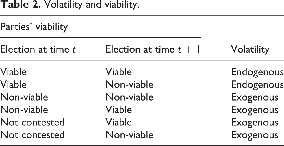
In Table 2, we represent the six possible scenarios of vote transfers among viable and non-viable parties in two consecutive elections and the difference between endogenous and exogenous volatilities. When voters act in accordance with the existing equilibrium in the party system (i.e. in the election in time t), volatility is endogenous; when voters are not (i.e. they support non-viable parties in the election in time t), volatility is exogenous.

Table 2.

Volatility and viability.

Parties’ viability		Volatility
Election at time t	Election at time t + 1	Volatility
Viable	Viable	Endogenous
Viable	Non-viable	Endogenous
Non-viable	Non-viable	Exogenous
Non-viable	Viable	Exogenous
Not contested	Viable	Exogenous
Not contested	Non-viable	Exogenous

In order to facilitate the comparability of data, party mergers and splits are coded following the rules proposed by Mainwaring and Zoco (2007: 173). When a party splits into two or more parties between two consecutive elections, we compare its results in the first election with those of its largest successor in the second. The smaller new splinter party is treated as if it had no votes in the first election. When two or more parties merge and create a new organization, we calculate volatility using the original party with the highest percentage of the vote.¹ Additionally, following Powell and Tucker (2014), for countries employing mixed proportional representation (PR) and single-member district electoral systems, we only use the party list component of the election result.² Finally, in those countries using run-off systems, we focus on the election results of the first round.

All measures of electoral volatility in an election should be calculated at the district level, as district-level vote transfers across districts can be cancelled out when aggregating votes nationally, and weighted by district size (number of voters). However, due to the availability of data, volatility is normally calculated using national election results. We thus follow two slightly different rules to determine which parties are in equilibrium at the district and national levels. First, at the district level, the M + 1 rule (Cox, 1997) in the first of the pair of elections considered is applied. In a single-member district, for instance, only two parties should be seriously in the running for the seat when there is Duvergerian equilibrium and three parties (the expected winner and two runners-up) when there is non-Duvergerian equilibrium.

When using national election results, we define as viable those parties that win at least one seat in the election at time t, while parties that win no seats are considered non-viable. By definition, parties that win seats are in equilibrium in at least one of the districts of the electoral system. This definition of viability creates two empirical problems which, however, are not very relevant when calculating endogenous and exogenous volatilities. First, it is possible for parties to be in equilibrium in a district but not to win any seats (i.e. being the first loser in a Duvergerian equilibrium). This is a highly unlikely scenario and clearly irrelevant to the calculation of endogenous and exogenous volatilities, as their potential support would be negligible. Second, parties winning seats in some districts are not necessarily viable in all districts. As they are considered as viable everywhere, endogenous and exogenous volatilities are overestimated and underestimated, respectively. This is exactly the same problem faced by the Pedersen index. The calculation of endogenous and exogenous volatilities is not dramatically affected. According to the data compiled by Guinjoan (2014) for 240 elections in 46 democratic countries, the electoral support of non-viable parties at the district level is quite small due to the strategic behaviour of parties and voters. In our cross-country empirical analysis, volatility is calculated on national-level data in order to make comparisons with existing indicators.

The main difference between our measures and those proposed by Powell and Tucker (2014) and Chiaramonte and Emanuele (2017) is that we capture the relevance of parties without using arbitrary party support thresholds. In contrast to Mainwaring et al. (2017), party age (i.e. the number of elections a party has taken part in) does not matter for us. The support of a non-viable party counts as exogenous volatility independently of its party age; for Mainwaring et al. (2017), it counts as extra-system volatility in the first election but as within-system volatility in the following elections.

In Tables 3 and 4, we show how our measures of endogenous and exogenous volatilities are calculated at the district and the national levels, respectively. The data are drawn from the 2011 and 2015 lower-house elections in Spain due to substantial changes in the party system. The district-level data come from Cádiz, an eight-seat district in 2011 and a nine-seat district in 2015.

Table 3.

Volatility in the 2011 and 2015 elections in the district of Cádiz.

	Vote shares (seats)		Volatility (%)
Party	2011	2015	Endogenous	Exogenous
PP	47.72 (5)	28.03 (3)	9.85
PSOE	33.23 (3)	28.28 (3)	2.48
IULV-CA	8.87	6.08	1.40
UpyD	4.86	0.57		2.15
PA	3.15			1.58
EQUO^a	0.71
PACMA	0.47	1.19		0.36
Eb	0.38			0.19
PCPE	0.18	0.12		0.03
HARTOS.ORG	0.15			0.08
ANTICAPITALISTAS	0.14			0.07
INTERNET	0.10			0.05
UCE	0.04			0.02
PODEMOS		20.43 (2)		9.86
C’s		14.84 (1)		7.42
VOX		0.23		0.12
RECORTES CERO		0.16		0.08
P-LIB		0.07		0.04
Total	100	100	13.72	22.03

Note: The number of seats won is in parenthesis. Viable parties at election in time t are in bold.

^a EQUO contested the 2015 election with Podemos. Support for the two parties is added together.

Table 4.

Volatility in the 2011 and 2015 elections in Spain.

Party (seats in time t)	Vote shares		Volatility (%)
Party (seats in time t)	2011	2015	Endogenous	Exogenous
PP (123 seats)	45.25	28.92	8.17
PSOE (90 seats)	29.16	22.16	3.50
IU-LV (2 seats)	7.02	3.70	1.66
UpyD	4.76	0.62	2.07
CiU ^a (8 seats)	4.23	2.27	0.98
EN MAREA ^b (PODEMOS)		1.63
AMAIUR ^c (2 seats)	1.39	0.88	0.26
EAJ-PNV (6 seats)	1.35	1.21	0.07
ERC (9 seats)	1.07	2.4	0.67
EQUO^b	0.9		0.9
BNG	0.77	0.28	0.25
CC-NC-PNC (1 seat)	0.6	0.33	0.14
COMPROMÍS-Q ^c (PODEMOS)	0.52
PACMA	0.43	0.88		0.23
FAC ^d (PP)	0.41
Eb	0.41	0.04		0.19
PA	0.32			0.16
PxC	0.25			0.13
PRC	0.18			0.09
GEROA BAI	0.17	0.12	0.03
PUM+J	0.11	0.02		0.05
PCPE	0.11	0.12		0.01
ANTICAPITALISTAS	0.09			0.05
PIRATA.CAT	0.09			0.05
UCE	0.07			0.04
PH	0.04	0.01		0.02
ESPAÑA 2000	0.04			0.02
SAIn	0.03	0.02		0.01
RPS	0.02			0.01
HARTOS.ORG	0.02			0.01
PIRATA	0.01			0.01
ANC	0.01			0.01
FE de las JONS	0.01	0.03		0.01
CDL	0.01			0.01
PCAS	0.01			0.01
UxV	0.01			0.01
P-LIB	0.01	0.01		0
PREPAL	0.01	0.01		0
POSI	0.01			0.01
DN	0.01	0.01		0
PRAO	0.01			0.01
Caballas	0.01			0.01
C.XXI	0.01			0.01
PODEMOS (69 seats)		20.83		9.97
C’s (40 seats)		14.05		7.03
Unió.cat		0.26		0.13
VOX		0.23		0.12
RECORTES CERO		0.19		0.10
MES		0.14		0.07
EL PI		0.05		0.03
CCD		0.04		0.02
SOMVAL		0.02		0.01
X LA IZQUIERDA		0.02		0.01
PUM+J		0.02		0.01
CENTRO MODERADO		0.01		0.01
PT		0.01		0.01
CANARIAS DECIDE		0.01		0.01
ARA. PV		0.01		0.01
EU-Ex		0.01		0.01
PCOE		0.01		0.01
Ifem		0.01		0.01
EZQUERRA		0.01		0.01
EN POSITIU		0.01		0.01
TOTAL	100	100	17.77	18.60

Note: Parties winning seats in the election at time t are in bold. The number of seats is in parenthesis.

^aCiU split into two parties in 2015: Democràcia i Llibertat and Unió Democrática de Catalunya (Unió.cat).

^b These two parties contested the 2015 election with Podemos. Support for the two parties is added to that for this party.

^c In 2015, EH Bildu.

^d It contested the 2015 election with the PP. Support for the two parties is added together.

As can be seen in Table 3, the total volatility in the district of Cádiz is 35.75%, while the endogenous and exogenous volatilities are 13.72 and 22.03%, respectively. According to Table 4, the total volatility in Spain is 36.37%; the exogenous volatility, 18.60%, is slightly higher than the endogenous volatility, 17.77%.

Describing endogenous and exogenous volatilities

Our sample includes 448 electoral cycles in lower-house elections in 66 countries in 4 regions (Western Europe, Eastern Europe, post-Soviet Union countries and the United States) between 1977 and 2011 (see Table 1A in the Online supplemental appendix). The analysis includes all independent states with a total population of 500,000 inhabitants or more and information available about election results. Following Mainwaring et al. (2017: 625), we have included countries whose polity score was 3 or higher in the years of the elections and all years in between. A polity score of 3 is designed to eliminate authoritarian regimes. We start at the end of the 1970s to include third- and fourth-wave democracies and have a fairly similar number of contemporaneous electoral cycles in every country.

The average endogenous and exogenous volatilities in our sample of countries are presented in Figure 1. The time mean of endogenous volatility is 12.9 and the standard deviation is 6.8, while the time mean of exogenous volatility is 5.3 and the standard deviation is 5.3. There are three interesting results. First, there are huge differences across countries. The average exogenous volatility ranges from 0.3 in Malta to 24.0 in Lithuania, while the average endogenous volatility extends from 2.04 in Malta to 36.7 in Sierra Leone. Second, with the exception only of South Korea and Bulgaria, endogenous volatility is greater than exogenous volatility in all the countries in the sample. Third, the relative weight of the two types of volatility differs greatly across countries. While in Colombia, for instance, the endogenous and exogenous volatility scores are very similar, in Finland endogenous volatility is about five times greater than exogenous volatility.

Figure 1.

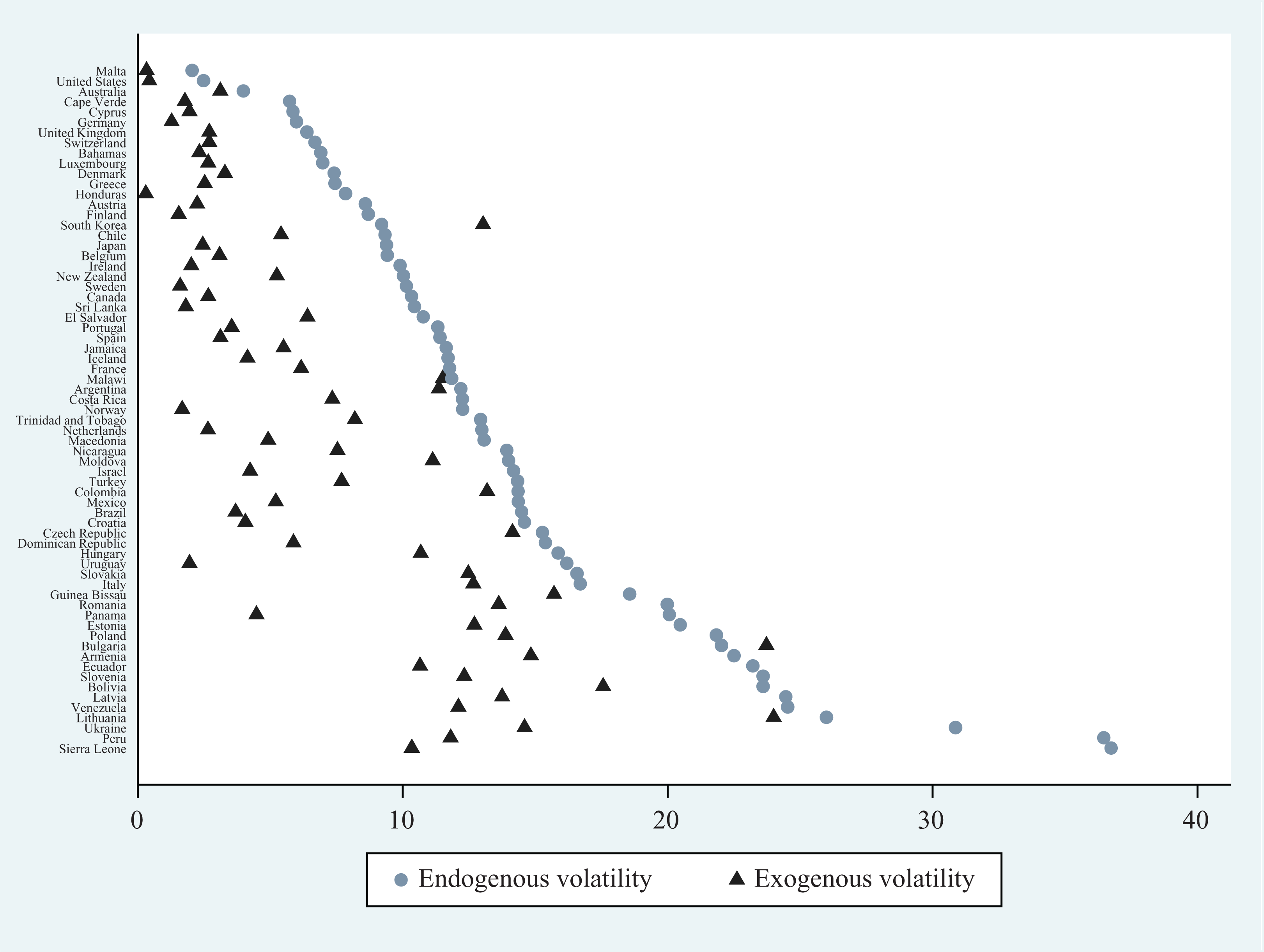
Endogenous and exogenous volatility in 66 countries (average 1977–2011).

Explaining cross-country and cross-temporal differences in the institutionalization of party systems

Two types of factors have been hypothesized to affect volatility: economic performance, in particular gross domestic product (GDP) growth and inflation, and institutional openness, that is, how permissive institutions are regarding the emergence of new parties. Volatility should increase the greater the district magnitude in the electoral system, the higher the number of parties, and in presidential regimes (Mainwaring et al., 2017). However, there are no clear hypotheses in existing research explaining why the two types of volatility are affected by the two groups of determinants and whether the effect should be observed across countries and/or over time. Not surprisingly, the empirical evidence is inconclusive.

According to Mainwaring et al. (2017: 628), both economic performance and institutional openness should affect both types of volatility, while Powell and Tucker (2014) argued that the government performance should explain both type A and type B volatilities, the number of parties should only affect type B volatility and formal institutional barriers should result in less type A volatility. Surprisingly, Mainwaring et al. found that different factors drive within- and extra-system volatility, but no explanation was provided for this unexpected result. On the other hand, Powell and Tucker found no support for the argument that institutional openness affects the levels of volatility, while economic performance is the only statistically significant predictor of type A volatility. When dropping the observations from Bosnia-Herzegovina, a clear outlier, none of the covariates has a statistically significant effect on the two types of volatility (Crabtree and Golder, 2017).

When volatility is examined in terms of electoral coordination theories, the hypotheses about the cross-national and cross-temporal effects of economic performance and institutional openness are clear. Whereas endogenous volatility reflects accountability, exogenous volatility captures the transaction costs for an alternative equilibrium in the party system. We derive two empirical expectations from this distinction. First, we hypothesize that government performance should only affect endogenous volatility, particularly with an economic decline and over time. According to ‘grievance asymmetry’ (Nannestad and Paldam, 1994), voters tend to punish poor economic performance more than they reward good economic performance. Economic performance, however, is not expected to affect exogenous volatility.

Second, our expectation is that institutional openness should have different effects on endogenous and exogenous volatilities. The electoral system, captured with the level of disproportionality, is the most important variable explaining the transaction costs for an alternative coordination. The less permissive the electoral system, the more stable the equilibrium. As a result, the electoral system is expected to affect exogenous volatility. The effect of disproportionality should be cross temporal. If the deviation between parties’ vote and seat shares increases, the reason is that small, non-viable parties are receiving more support. As countries with majoritarian electoral systems are not inherently more institutionalized than countries with PR, we do not expect to find a cross-country effect of disproportionality on exogenous volatility. Everything else being equal, we have no reason to expect that incumbents are more or less accountable in majoritarian than in PR systems. Electoral disproportionality thus should not affect endogenous volatility cross-nationally.

Following Powell and Tucker (2014: 134), we expect that party system fragmentation will increase the endogenous volatility from both a cross-country and a cross-temporal perspective; the more viable the parties are, the more opportunities there are for party switching. On the other hand, we expect that the greater the effective number of parties in a country, the greater the exogenous volatility. However, there is no clear prediction about how changes in the effective number of parties influence exogenous volatility; it is not possible to determine whether the greater dispersion of votes across parties is due to the emergence of new parties or simply the redistribution of partisan support between viable parties.

Finally, as equilibria are not affected by political regimes and there are no reasons to expect that governments are more (or less) accountable in presidential than in parliamentary regimes, this variable should not affect volatility.

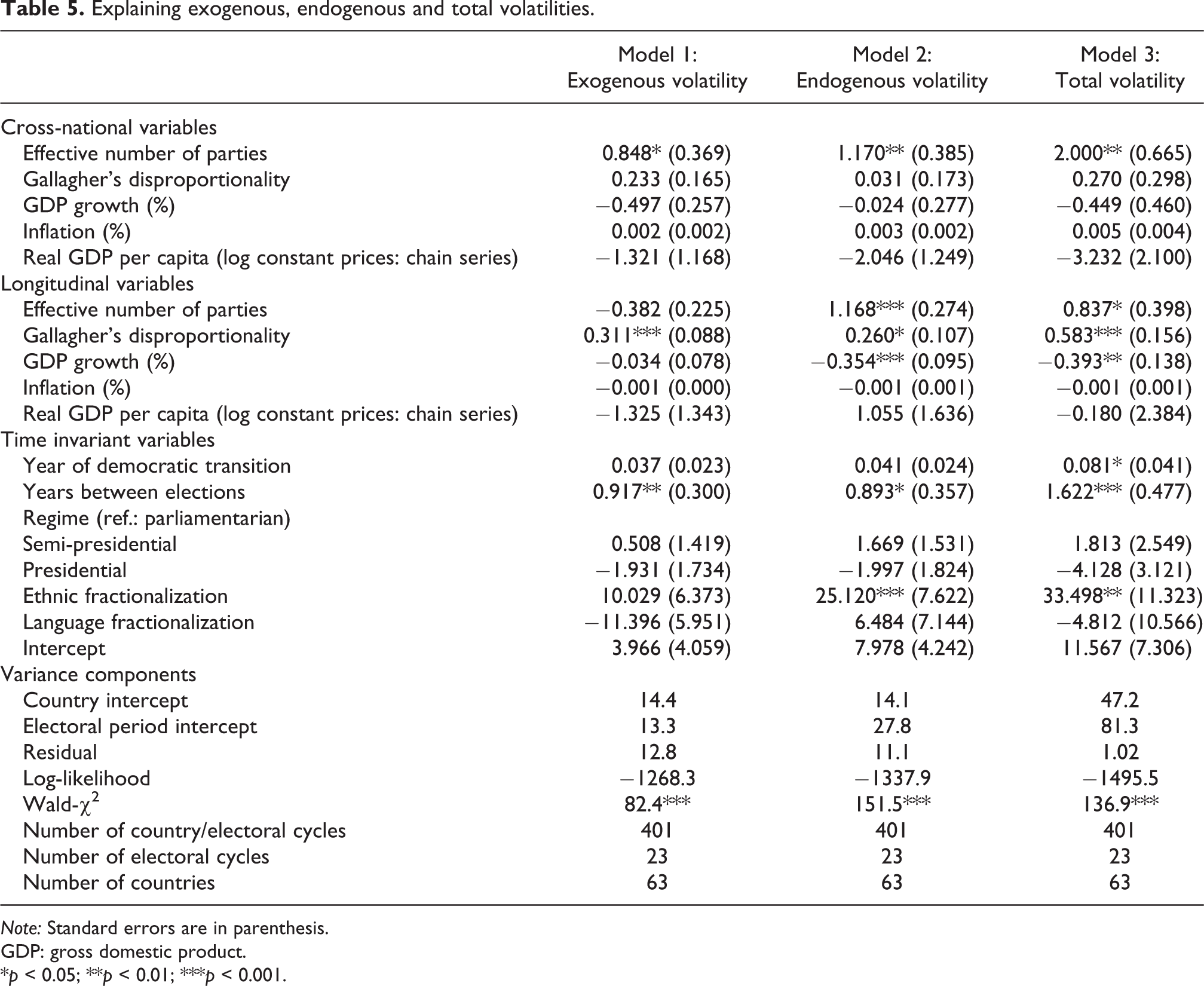
In Table 5, we rely on data from 63 countries and 401 electoral cycles in lower-house elections between 1977 and 2011 to examine the determinants of exogenous, endogenous and total volatilities.³ The inclusion of some variables in the models could be disputed, but the intention is replicating models from preceding studies, especially the most exhaustive one presented by Mainwaring et al. (2017). The economic performance argument is captured with three time-variant variables: country per capita income,⁴ inflation⁵ and economic growth.⁶ The institutional openness argument is operationalized using the effective number of electoral parties,⁷ Gallager’s index of electoral disproportionality,⁸ the political regime⁹ and the year of the creation of the current democratic system.¹⁰ The last two variables are time invariant. Finally, we control for ethnic fractionalization and linguistic fractionalization indices,¹¹ the number of years between elections and a linear time variable. The descriptive statistics of the variables are presented in Table 1B of the Online supplemental appendix. Additionally, to deal with the potential problem of endogeneity, all the independent variables are measured during the election at time t of the electoral cycle. The only exception is Gallagher’s index of disproportionality, since we consider voters taken into consideration at the moment of t + 1.

Table 5.

Explaining exogenous, endogenous and total volatilities.

	Model 1: Exogenous volatility	Model 2: Endogenous volatility	Model 3: Total volatility
Cross-national variables
Effective number of parties	0.848* (0.369)	1.170** (0.385)	2.000** (0.665)
Gallagher’s disproportionality	0.233 (0.165)	0.031 (0.173)	0.270 (0.298)
GDP growth (%)	−0.497 (0.257)	−0.024 (0.277)	−0.449 (0.460)
Inflation (%)	0.002 (0.002)	0.003 (0.002)	0.005 (0.004)
Real GDP per capita (log constant prices: chain series)	−1.321 (1.168)	−2.046 (1.249)	−3.232 (2.100)
Longitudinal variables
Effective number of parties	−0.382 (0.225)	1.168*** (0.274)	0.837* (0.398)
Gallagher’s disproportionality	0.311*** (0.088)	0.260* (0.107)	0.583*** (0.156)
GDP growth (%)	−0.034 (0.078)	−0.354*** (0.095)	−0.393** (0.138)
Inflation (%)	−0.001 (0.000)	−0.001 (0.001)	−0.001 (0.001)
Real GDP per capita (log constant prices: chain series)	−1.325 (1.343)	1.055 (1.636)	−0.180 (2.384)
Time invariant variables
Year of democratic transition	0.037 (0.023)	0.041 (0.024)	0.081* (0.041)
Years between elections	0.917** (0.300)	0.893* (0.357)	1.622*** (0.477)
Regime (ref.: parliamentarian)
Semi-presidential	0.508 (1.419)	1.669 (1.531)	1.813 (2.549)
Presidential	−1.931 (1.734)	−1.997 (1.824)	−4.128 (3.121)
Ethnic fractionalization	10.029 (6.373)	25.120*** (7.622)	33.498** (11.323)
Language fractionalization	−11.396 (5.951)	6.484 (7.144)	−4.812 (10.566)
Intercept	3.966 (4.059)	7.978 (4.242)	11.567 (7.306)
Variance components
Country intercept	14.4	14.1	47.2
Electoral period intercept	13.3	27.8	81.3
Residual	12.8	11.1	1.02
Log-likelihood	−1268.3	−1337.9	−1495.5
Wald-χ ²	82.4***	151.5***	136.9***
Number of country/electoral cycles	401	401	401
Number of electoral cycles	23	23	23
Number of countries	63	63	63

Note: Standard errors are in parenthesis.

GDP: gross domestic product.

*p < 0.05; **p < 0.01; ***p < 0.001.

As we have a time-series cross-national aggregate panel data set, the estimation requires a three-level multilevel regression model in which country years (k) are nested within election cycles (i), which in turn are nested within countries (j)

y_{k i j} = β_{0} + β_{1} t_{k i j} + β_{2} x_{k i j} + β_{3} x_{i j} + β_{4} x_{i} + µ_{i} + µ_{i j} + e_{t i j}

where y_kij is the response variable of country j measured at election i on occasion k. x_kij is a time-varying covariate, such as GDP growth, while x_ij refers to a variable that varies between elections, such as the effective number of electoral parties (ENEP), but does not vary within a given election cycle. x_j denotes time- and election-cycle-invariant covariates, such as the type of the executive or the degree of ethnic fractionalization. Finally, t_kij refers to a linear time trend variable that captures the measurement occasion.

The above model is also referred to as a random-effects (RE) model. It makes the assumption that the errors µ_j are uncorrelated with the explanatory variables for all the time periods. For this reason, it is sometimes argued that a fixed-effects (FE) model should be preferred when dealing with time-series data, since it allows for a correlation between the residuals and the explanatory variables. However, with an FE model, it is impossible to test the effects of time-invariant variables. A similar problem arises in the context of rarely changing variables (Plümper and Troeger, 2007). Consequently, an FE model makes use of only a small part of the variation in a time-varying variable, since any higher-level variance is eliminated. Additionally, only the ‘within’ effects can be estimated, so nothing is known about the cross-sectional ‘between’ effects, which is also a major additional problem in the preceding literature when estimating the predictors of party system institutionalization. Bell and Jones (2015) and Schmidt-Catran and Fairbrother (2016) solved this problem by modelling the cross-sectional and longitudinal relationships simultaneously by adding a group mean and a demeaned term together in the model. This leads to the following ‘within–between’ RE model:

y_{t i j} = β_{0} + β_{1} t_{k i j} + β_{2} x_{k i j M} + β_{3}_{j} + β_{4} x_{i j M} + β_{5}_{j} + β_{6} x_{j} + µ_{i} + µ_{i j} + e_{k i j}

where the original time-varying variable x_kij and the election-varying variable x_ij are included twice in the model, decomposed into $\bar{x}$ _j and x_kijM and x_kijM , respectively. A benefit of this approach is that the ‘within’ coefficients will return the same results as in an FE model. Therefore, we can exclude the possibility that some unobserved time-invariant variables at the higher level are biasing the ‘within’ coefficients. Of equal importance is that this approach allows the estimation of the cross-sectional association between time-varying variables x and y, while it enables us to include time-invariant variables simultaneously in the model.

When explaining exogenous volatility (model 1 in Table 5), apart from the number of years between elections, the only two statistically significant variables (at the level of 0.05 and 0.001%, respectively) are the effective number of parties (the greater the number of competitors, the less stable the equilibrium) and the degree of disproportionality (when disproportionality increases over elections, the equilibrium becomes less stable).¹² As expected, institutional openness, in particular the electoral system, makes a difference to the institutionalization of the party system, while economic performance does not. In the second model, exogenous volatility is replaced with endogenous volatility as the dependent variable. Again in line with our hypotheses, endogenous volatility is driven by the number of parties (both cross-nationally and cross-temporally) and above all by GDP growth; the more options voters have to support and the worse a country is performing, the greater the number of vote transfers between or towards viable parties. The variables are statistically significant at the level of 0.01/0.001 and 0.001%. The economic performance argument is strongly supported. Finally, as endogenous volatility is greater than exogenous volatility in most of the countries, the determinants of total and endogenous volatilities are similar.

To show that the obtained results are not simply artefacts of our methods and data, and the inconsistent results of the existing measures of patterns of party system competition, we run the same models for extra-system (Mainwaring et al., 2017), regeneration (Chiaramonte and Emmanuele, 2017) and type A (Powell and Tucker, 2014) volatility with exactly the same methods. That is, after matching countries and electoral cycles, we combine our data set with the other ones including the variables of the three volatility scores as measured by the corresponding authors.

The results of the estimates are presented in Table 6. Interestingly, they are not robust across the three measures; that is, they do not capture the same phenomenon. If we focus first on the institutional openness argument, cross-national differences in electoral disproportionality only significantly affect regeneration volatility; however, when examining changes over time in electoral disproportionality, extra-system volatility is influenced by the electoral system. The number of parties positively affects regeneration and type A volatilities cross-nationally, but the effect of this variable over time is negative for extra-system volatility, positive for regeneration volatility and statistically insignificant for type A volatility. Finally, regeneration volatility is greater in presidential regimes than in parliamentary ones, while political regimes do not affect extra-system and type A volatilities. When examining the economic performance argument cross-nationally, GDP growth only influences regeneration volatility cross-nationally, while both regeneration and type A volatility increase with inflation. Extra-system volatility is not affected by economic performance. However, GDP growth (no inflation) increases extra-system volatility over time but has no effect on regeneration and type A volatilities.

Table 6.

Explaining extra-system, regeneration and type A volatilities.

	Model 4: Extra-system volatility	Model 5: Regeneration Volatility	Model 6: Type A volatility
Cross-national variables
Effective number of parties	0.378 (0.578)	0.547*** (0.151)	4.778*** (0.848)
Gallagher’s disproportionality	0.142 (0.261)	0.158*** (0.042)	0.106 (0.367)
GDP growth (%)	0.742 (0.640)	0.662** (0.202)	1.273 (0.940)
Inflation (%)	0.005 (0.004)	0.132*** (0.039)	0.073** (0.028)
Real GDP per capita (log constant prices: chain series)	−4.400 (2.519)	1.963* (0.797)	−9.463** (3.137)
Longitudinal variables
Effective number of parties	−1.835*** (0.556)	1.543*** (0.246)	0.630 (0.855)
Gallagher’s disproportionality	0.787*** (0.189)	0.033 (0.085)	0.193 (0.467)
GDP growth (%)	−0.439* (0.188)	−0.024 (0.060)	0.174 (0.293)
Inflation (%)	−0.001 (0.001)	−0.005 (0.022)	0.004 (0.010)
Real GDP per capita (log constant prices: chain series)	11.703** (4.271)	−2.218** (0.739)	−17.069** (5.890)
Time invariant variables
Year of democratic transition	2.473 (2.581)	−0.534 (0.417)	−1.428 (2.703)
Years between elections	−4.639 (3.038)	2.155* (1.059)	−2.249 (7.777)
Regime (ref.: parliamentarian) semi-presidential	5.033 (6.452)	−9.294*** (2.342)	−19.172 (16.447)
Presidential	3.365 (6.878)	8.302*** (1.768)	13.843 (14.554)
Ethnic fractionalization	−35.713 (97.588)	−81.238*** (23.979)	−61.232 (118.799)
Language fractionalization	2.473 (2.581)	−0.534 (0.417)	−1.428 (2.703)
Intercept	−4.639 (3.038)	2.155* (1.059)	−2.249 (7.777)
	5.033	−9.294***	−19.172
Variance components
Country intercept	20.7	0.00	17.1
Time intercept	0.82	0.00	1.8
Residual	99.4	2.9	95.7
Log-likelihood	−1087.6	−304.2	−532.0
Wald-χ ²	78.5***	92.4***	146.6***
Number of country/electoral cycles	53	19	33
Number of electoral cycles	29	33	23
Number of countries	287	156	141

Note: Standard errors are in parenthesis.

GDP: gross domestic product.

*p < 0.05; **p < 0.01; ***p < 0.001.

Conclusions

After re-examining Powell and Tucker’s (2014) results and finding no variables with a statistically significant effect on either type A or type B volatility, Crabtree and Golder (2017: 234) claimed that ‘this area of research cries out for a new theoretical development’. Filling this crucial gap has been the goal of this article.

We have built on electoral coordination theories to disaggregate volatility into its exogenous and endogenous components. The former captures how many voters are not acting in accordance with the existing equilibrium in the party system. The greater the number of vote transfers between or towards parties that are not in equilibrium, the greater the likelihood of a coordination failure and then a realignment. On the other hand, endogenous volatility captures the volatility between or towards those parties that are in equilibrium. Endogenous volatility is positive for representative democracies; if the distribution of partisan support across parties does not change between two consecutive elections or the change is minimal, incumbents do not face incentives to be representative. Thus, endogenous volatility reflects the stability of the party system equilibrium, while endogenous volatility measures the stability of the distribution of partisan support across viable parties or parties that are in equilibrium.

This new theoretical development has two advantages over the existing measures of volatility. First, it is based on a simple and theoretically robust rule for counting parties: electoral viability according to Cox’s M + 1 rule. As a result, ad hoc or arbitrary decisions, such as party age or partisan support, are no longer necessary to calculate the two types of volatility, and spatial and longitudinal comparisons are straightforward. Second, when volatility is examined in terms of electoral coordination theories, clear hypotheses about the determinants of cross-national and cross-temporal changes can be formulated. While government performance affects endogenous volatility, exogenous volatility is a function of institutional openness.

Supplemental Material

Supplemental Material, sj-docx-1-ppq-10.1177_1354068818795191 - Electoral coordination and party system institutionalization

Supplemental Material, sj-docx-1-ppq-10.1177_1354068818795191 for Electoral coordination and party system institutionalization by Ignacio Lago and Mariano Torcal in Party Politics

Footnotes

Declaration of Conflicting Interests

The authors declared no potential conflicts of interest with respect to the research, authorship, and/or publication of this article.

Funding

The authors disclosed receipt of the following financial support for the research, authorship, and/or publication of this article: This work was supported by the Ministerio de Economıía y Competitividad of Spain under the research project CSO2017-85024-C2-1-P and ICREA.

ORCID iD

Mariano Torcal

Supplemental Material

Supplemental material for this article is available online.

Notes

References

Aldrich

(2011) Why Parties? A Second Look. Chicago: Chicago University Press.

Alesina

Devleeschauwer

Easterly

, et al. (2003) Fractionalization. Journal of Economic Growth 8: 155–194.

Bell

Jones

(2015) Explaining fixed effects: random effects modeling of time-series cross-sectional and panel data. Political Science and Research Methods 3: 133–153.

Bormann

N-C

Golder

(2013) Electoral systems around the world: 1946-2011. Electoral Studies 32: 360–369.

Casal-Bertoa

Deegan-Krause

Haughton

(2017) The volatility of volatility: measuring change in party vote shares. Electoral Studies 50: 142–156.

Cheibub

Jennifer

Vreeland

(2010) Democracy and dictatorship revisited. Public Choice 143: 67–101.

Chiaramonte

Emanuele

(2017) Party system volatility, regeneration and de-institutionalization in Western Europe (1945-2015). Party Politics 23: 376–388.

Chhibber

Kollman

(2004) The Formation of National Party Systems: Federalism and Party Competition in Canada, Great Britain, India, and the United States. Princeton: Princeton University Press.

Cox

(1997) Making Votes Count: Strategic Coordination in the World’s Electoral Systems. New York: Cambridge University Press.

10.

Crabtree

Golder

(2017) Party system volatility in post-communist europe. British Journal of Political Science 47: 229–234.

11.

Gallagher

(2017) ‘Election Indices Dataset’, Available at: https://www.tcd.ie/Political_Science/staff/michael_gallagher/ElSystems/Docts/ElectionIndices.pdf (accessed on 1 May 2017).

12.

Guinjoan

(2014) Parties, Elections and Electoral Contests: Competition and Contamination Effects. Surrey: Ashgate.

13.

Key

(1964) Politics, Parties, and Pressure Groups. New York, NY: Crowell.

14.

Mainwaring

Timothy

(1995) Building Democratic Institutions: Party Systems in Latin America. Stanford: Stanford University Press.

15.

Mainwaring

Torcal

(2006) Party system institutionalization and party system theory after the third wave of democratization. In: Richard

Crotty

(eds) Handbook of Party Politics. Thousand Oaks: Sage, pp. 204–227.

16.

Mainwaring

Zoco

(2007) Political sequences and the stabilization of interparty competition: electoral volatility in old and new democracies. Party Politics 13: 155–178.

17.

Mainwaring

Gervasoni

España-Nájera

(2017) Extra- and within-system electoral volatility. Party Politics 23: 623–635.

18.

Nannestad

Paldam

(1994) The VP-function: a survey of the literature on vote and popularity functions after 25 years. Public Choice 79: 213–245.

19.

Pedersen

(1979) The dynamics of European party systems: changing patterns of electoral volatility. European Journal of Political Research 7: 1–26.

20.

Pedersen

(1983) Changing patterns of electoral volatility in European party systems, 1948-1977: explorations in explanation. In: Hans

Mair

(eds) Western European Party Systems: Continuity and Change. Beverly Hills: Sage, pp. 29–66.

21.

Plümper

Troeger

(2007) Efficient estimation of time-invariant and rarely changing variables in finite sample panel analyses with unit fixed effects. Political Analysis 15: 124–139.

22.

Powell

Tucker

(2014) Revisiting electoral volatility in post-communist countries: new data, new results and new approaches. British Journal of Political Science 44: 123–147.

23.

Sanchez

(2009) Party non-systems. A conceptual innovation. Party Politics 15: 487–520.

24.

Schleiter

Voznaya

(2016) Party system institutionalization, accountability and governmental corruption. British Journal of Political Science 48: 315–342.

25.

Schmidt-Catran

Fairbrother

(2016) The random effects in multilevel models: getting them wrong and getting them right. European Sociological Review 32: 23–38.

26.

Tavits

(2008) On the linkage between electoral volatility and party system instability in Central and Eastern Europe. European Journal of Political Research 47: 537–555.

27.

Teorell

Dahlberg

Holmberg

, et al. (2015) The Quality of Government Standard Dataset, version 15 January. University of Gothenburg: The Quality of Government Institute, Available at: http://www.qog.pol.gu.se (accessed on 15 May 2018).

28.

Weghorst

Bernhard

(2014) From formlessness to structure? The institutionalization of competitive party systems in Africa. Comparative Political Studies 47: 1707–1737.

Supplementary Material

Please find the following supplemental material available below.

For Open Access articles published under a Creative Commons License, all supplemental material carries the same license as the article it is associated with.

For non-Open Access articles published, all supplemental material carries a non-exclusive license, and permission requests for re-use of supplemental material or any part of supplemental material shall be sent directly to the copyright owner as specified in the copyright notice associated with the article.

0.00 MB

0.03 MB