Application of PCA with georeferenced data in the tourism industry: A case study in the province of Córdoba,Argentina

Abstract

The spatial analysis of tourism industries provides information about their structure, which is necessary for decision-making. In this work, tourism industries in the departments of Córdoba province, Argentina, for the 2001–2014 period were mapped. Multivariate methods with and without spatial restrictions (spatial principal components (sPCs) analysis, MULTISPATI-PCA, and principal components analysis (PCA), respectively) were applied and their performance was compared. MULTISPATI-PCA yielded a higher degree of spatial structuring of the components that summarize tourism activities than PCA. The methodological innovation lies in the generation of statistics for multidimensional spatial data. The departments were classified according to the participation of tourism activities in the value added of tourism using the sPCs obtained as input of the cluster fuzzy k-means analysis. This information provides elements necessary for appropriately defining local development strategies and, therefore, is useful to improve decision-making.

Keywords

cluster fuzzy k-means spatial multivariate analysis tourism industries

Introduction

The analysis of tourism industries allows us to generate information about their structure; this information provides elements necessary for appropriately defining local development strategies and, therefore, is useful to improve decision-making. Tourism plays an important role in the economy of a region, since it has a multiplier effect on production, employment, and income. In Córdoba province, Argentina, tourism has been indicated as one of the strategic sectors of economic development (Córdoba Tourism Agency, 2019). Moreover, there is an interest of policy makers in identifying development areas and regions with the aim of planning the infrastructure, improving transport, develop tourist products, and satisfactorily manage the social, environmental, and cultural impacts of tourism.

Works exploring economic data may require the incorporation of geographical references to identify and explain spatial variability of economic structures. The importance of methods that analyze spatial effects on economic models has increased notably in the last years, partly due to the renewed interest in the role of space and spatial interaction in economic theory; this topic has been incorporated in some works, such as those of the new economic geography (Krugman, 1998). Furthermore, availability of new statistical sources of microterritorial data (census data, directories, etc.) as well as improved computer application tools and development of specific software for the treatment of spatial data (Anselin and Florax, 1995) have originated an increasing demand for this type of spatial analysis.

The analysis of space is gaining special importance in the social sciences, especially tourist activities due to their close relationship with a given territory.

In recent years, methods for the study of regional economy have been widely developed due to the need to work on the so-called spatial effects: heterogeneity and spatial dependence. Spatial heterogeneity consists of the variation of relationships in space; it refers to the lack of spatial stability of the behavior of studied the variable. This implies, for example, that the functional form and the parameters of a regression may vary among locations, being therefore not homogeneous throughout the sample. On the other hand, spatial dependency or autocorrelation occurs when the value of a variable at one site in space is related to its value in another or other sites in space. This work focuses on spatial dependency. The identification and measurement of spatial structures is an important issue in tourist activities.

A literature review in the tourism field suggests that there is an increasing demand for studies that analyze the spatial pattern of tourist activities in order to obtain comprehensive information for the proper management and planning of the activities at the destinations. Some empirical studies have identified the spillover effects in tourist flows and regional growth (Capone and Boix, 2008; Gooroochurn and Hanley, 2005; Lazzeretti and Capone, 2009; Neumayer, 2004; Rodríguez Rangel et al., 2020; Yang and Wong, 2013). Yang and Fik (2014) examined two particular spatial effects on regional tourism growth: spatial spillover and spatial heterogeneity. Yang and Wong (2013) investigated the spatial distribution of inbound and domestic tourist flows to cities in China and their growth rates using exploratory spatial data analysis, and showed that tourism flows are polarized into clusters and remain very stable over time. In addition, several studies have focused on identifying and characterizing localized clusters (Chhetri et al., 2013; Rodríguez Rangel et al., 2020).

In the field of tourism, one of the main difficulties in spatial analysis is the integration of the analysis units (municipalities, departments, etc.) in broader regional structures (Hall, 2005). In this article, we build on an innovative approach to multidimensional spatial data statistics and cluster identification.

Two multivariate techniques (principal component analysis (PCA) and spatially restricted PCA) are applied. The results obtained with the implementation of a classic PCA and the spatially restricted version (MULTISPATI-PCA) were comparatively analyzed. Then, the spatial main components obtained with MULTISPATI-PCA were used as input to the fuzzy k-means cluster analysis for the identification of homogeneous groups of departments. The hypothesis underlying the proposed methodology is that the incorporation of spatial autocorrelation through the spatial PCA applied to the tourism characteristic activities obtained at the department level will group departments according to homogeneity and spatial coherence.

Multivariate analysis methods are used to summarize data sets into new variables built by transforming the original ones, with a minimum loss of information. PCA (Pearson, 1901), one of the outstanding multivariate analysis methods, allows us to identify the variables that account for the greatest total variability of the data, explore the correlations among variables, and reduce the dimension of the analysis by combining the variables into new indices (synthetic variables). Each one of these new synthetic variables is termed principal component (PC). Standard multivariate techniques can be successfully applied to data sets for which there is information about the spatial location of each unit of analysis (georeferenced data). In these cases, synthetic variables are usually obtained and then their spatial variation is described to obtain contour maps related to the new index variables. However, this type of analysis does not take into account the spatial relationships directly in the estimation of the components; ordination techniques, such as PCA, were not designed specifically to identify spatial structures. Geographical information is usually incorporated after performing the PCA, by assigning the values of the components to each of the georeferenced sites or by adjusting semivariograms and using other tools of classical geostatistics (kriging) to generate spatial variability maps through interpolation.

The presence of spatial autocorrelation of the PCs can be detected using univariate autocorrelation statistics, such as Moran’s index (MI, Moran, 1948) or Geary’s index (Geary, 1954). These analyses are conducted using a univariate approach, which hinders interpretation of the total variability (Córdoba et al., 2012). Dray et al. (2008) proposed MULTISPATI-PCA, a multivariate analysis method that incorporates spatial information prior to the multivariate analysis. This method is based on PCA but incorporates the restriction given by the spatial data by calculating the MI to measure dependence or spatial correlation between observations at a site and the mean of observations in the neighborhood of that site. The neighborhood is delimited using a spatial weights matrix, determining which and how many observations near each site make up the neighborhood (Córdoba et al., 2013).

This article is structured as follows: After this introduction we then proceed to characterize the destination under study (“Case study: Córdoba (Argentina)” section). In the methodology section, the statistical techniques used PCA-MULTISPATI (“Application of PCA and sPCA” section) and fuzzy k-means (“Multivariate site classification” section) are described; then the main results obtained in with each method are presented (“Results and discussion” section). Finally, the main conclusions and implications of the results of this research are explained.

Case study: Córdoba (Argentina)

Córdoba province, located in the geographical center of Argentina (Figure 1), with a surface area of 165,321 km² and a population of 3,304,825 inhabitants (INDEC, 2010) is the second most populated province after the province of Buenos Aires. Córdoba is a vast territory that comprises plains, mountain ranges, and valleys, generating the provincial landscape identity. The mountain area harbors abundant water bodies (rivers, streams, springs, lakes, lagoons, and reservoirs) that together with the mountains make up Córdoba’s traditional tourist attraction. The mild climate of the province, of continental type with cool winters and warm summers, makes the territory a tourist destination throughout the year. Córdoba is the second most important tourist destination in Argentina after the Atlantic coast in the province of Buenos Aires. Córdoba is mainly a domestic destination; indeed, more than 90% of visitors are Argentinians, with prevalence of families and the middle-income sector (MINTUR, 2012). Córdoba region stands out for the tourist movement given the number of visitors and the accommodation capacity, with about 1.5 million hotel beds available per month on average (INDEC, EOH, 2018). Comparing with Comparing Córdoba with other of the main tourist destinations in Argentina, it is observed that Córdoba has an important hotel sector. The monthly average of available hotel rooms in Córdoba is five times that of Mendoza, four times that of Salta and three times that of Bariloche, three other important Argentine tourist destinations. Considering the number of visitors hosted per year, in 2017, Córdoba received about four times more visitors than Mendoza and three times more than Salta and Bariloche.

Figure 1.

Location of the province of Córdoba in Argentina. Maps: Córdoba Tourism Agency, Province of Córdoba.

Methods

Data

The data used for this study, corresponding to the province of Córdoba and its 26 departments, were obtained from the Department of Statistics and Censuses of the province of Córdoba for the 2001–2014 period. We worked with the gross geographical product series at constant values, because it presents greater stability than at current values and allows us to analyze the economic structure.

Prior to the analysis, the data were subjected to a depuration procedure. First, the tourism industries (UNWTO, 2010) for which there was information in all the departments were selected. The following activities were considered: (1) hotels (H), (2) second homes tourism (SH), (3) food and beverage serving services (FB), (4) road passenger transport (RT), (5) travel agencies (TA), (6) cultural activities (CA), and (7) sports activities (SA) and other recreational activities. The data were normalized by calculating relative shares, defined as the quotient between the value of the specific activities and the total value added of each department; this allows us to work with the composition of the activity and avoids the differences that arise in absolute values (monetary) because of the different economy sizes among departments.

Given the lack of significant differences of PCA results among years, we decided to use the average value for the period (2001–2014).

Application of PCA and sPCA

The main objective of the PCA is to describe a data matrix, reduce the number of variables that explain the main variations, and identify correlations between the measured variables to generate new uncorrelated variables (i.e. easy to interpret), called main components. The PCA consists of finding orthogonal transformations of the original variables to get a new set of variables that are not correlated. The PCA explains the total of the variability of the data; to obtain an effective reduction in its dimension it is necessary that the variables are correlated. The components are linear combinations of the original variables and it is expected that only a few (the first ones) will collect most of the variability of the data, obtaining a reduction in the dimension of the data. In summary, the PCA finds the weights or weights for each variable in order to construct linear combinations of variables capable of maximizing the variance between the sampling areas. The linear combinations obtained (PCs) are orthogonal (independent) and together they explain all the variability of the original data. The first component (PC1) explains most of the total variation in the data set and the second (PC2), most of the variability remaining or not explained by PC1. Therefore, the fundamental purpose of the technique is to reduce the size of the data in order to simplify the study problem.

The results of the PCA are illustrated in a graph called Biplot (Gabriel, 1971), which represents in an optimal plane for the study of variability, the differences between sites, the correlation between variables, and the variables that best explain the main variations. The incorporation of the geographic information or the spatial characteristics of the data can be done after doing the PCA, by assigning the values of the components to each of the georeferenced sites or by adjusting semivariograms to the PC. An advantage of using synthetic variables for mapping is that the multidimensional characterization of the observations collapses, allowing the construction of synthetic maps of spatial variability. This technique allows us to visualize the pattern of spatial variability and graphically explore the spatial structure of the analyzed variables. The presence of spatial autocorrelation in PCs can also be studied using univariate autocorrelation statistics such as the MI (Moran, 1948) or the Geary index (Geary, 1954). These indices are used to measure and analyze the degree of dependency between observations in a geographic context (Cliff and Ord, 1973). Multivariate data are generally recorded in an X matrix with n rows (observations) and p columns (variables). The duality diagram provides a theoretical framework that defines the structure of numerous multivariate analysis methods using three matrices (X, Q, D). Duality diagram theory includes standard methods such as PCA and its extension to spatial data. The data matrix X (n × p; original or transformed) is considered part of the triplet (X, Q, D), where $Q_{p \times p}$ and $D_{n \times n}$ are usually positive definite symmetric matrices used as relationship or distance metrics.

To carry out the spatially restricted PCA, called MULTISAPTI-PCA, it is first necessary to define how the spatial information is entered into the analysis. In MULTISAPTI-PCA, the spatial structure is detected using the MI. This approach then requires the definition of neighboring sites. This is generally achieved by the construction of a connection network (also called neighbor graphics), which uses objective criteria to define which entities are neighbors and which are not. There are different options or methodological alternatives to define the neighborhoods that depend on the different types of sampling present in the data (regular, irregular, or transect grid) (Bivand, 2008). For irregular samplings, the methods are based on the Gabriel graph (Gabriel and Sokal, 1969), the Delaunay triangulation (Lee and Schachter, 1980), the closest neighbors, and the Euclidean distance, among others. There are different options or methodological alternatives to define the neighborhoods that depend on the different types of sampling present in the data (regular, irregular, or transect grid). For irregular samplings, the methods used to build the connection network are based on Delaunay triangulation (Lee and Schachter, 1980), the Gabriel graph (Gabriel and Sokal, 1969), the concept of closest neighbors, and Euclidean distance between observations. When irregular areas are involved, a point is usually chosen to represent the polygon, often referred to as the centroid of the polygon. The different methods are shown in Figure 2. Delaunay triangulation is a recommended method for constructing neighborhood charts when features are evenly distributed in space. However, it is possible to connect to peripheral entities that should not be related. Gabriel’s graph is a subset of Delaunay’s graph that does not include peripheral connections.

Figure 2.

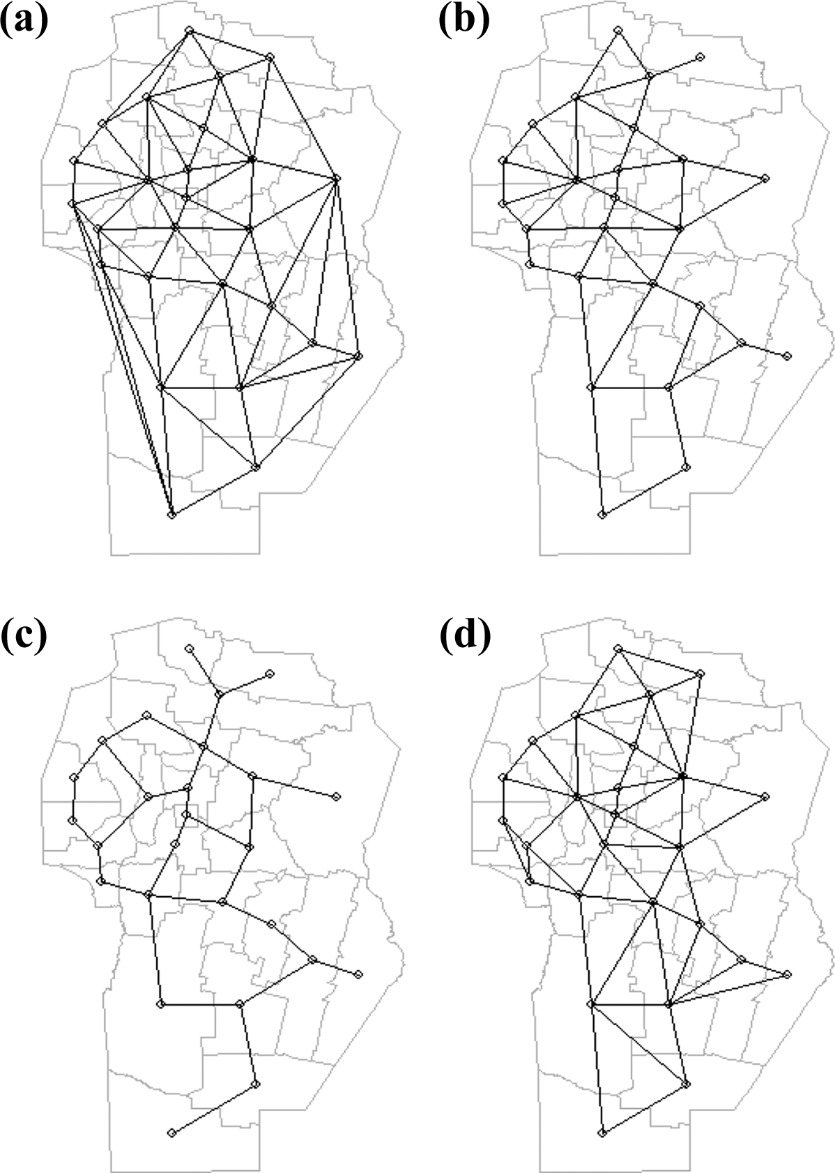
(a) Delaunay triangulation neighbors; (b) Gabriel graph neighbors; (c) relative graph neighbors; (d) sphere of influence graph.

Once the connection network is defined, the spatial information is stored in a binary connection matrix (in which if the spatial units are neighboring, it assumes the value 1 or 0 otherwise), which is symmetric and its rows and columns correspond to the same entity (as a distance matrix). This general connectivity matrix is scaled to obtain the spatial weights matrix W. The matrix is a mathematical representation of the geographical arrangement of the points in the region (Bivand, 2008). The spatial weights reflect a priori the absence or presence (intensity) of the spatial relationship between the locations of interest. Once the spatial weights have been defined, the autocorrelation index MI is computed. The MULTISPATI-PCA method introduces a standardized spatial weight matrix (W) per row by means of statistical triplet analysis (X, Q, D). The matrix $\tilde{X} = W X$ is composed of the weighted averages of the values of the neighbors according to the spatial connection matrix; it is called the lagged matrix. The two tables X and $\tilde{X}$ have the same columns (variables) and the same rows (observations). The MULTISPATI-PCA consists of the analysis of this pair of tables (X and $\tilde{X}$ ) by means of a coinercia analysis (Dray et al., 2003). To establish the statistical significance of the spatial structure of the table, a permutation-based procedure can be used. The statistic used is equal to the trace $(X^{T} D W X Q)$ . The p value is computed by comparing the observed value to those obtained by permutation of the rows of X (Córdoba et al., 2012). MULTISPATI-PCA maximizes the dot product between a linear combination of the original variables and a linear combination of lagged variables (Saby et al., 2009). The advantage of MULTISPATI-PCA over PCA is that the spatial major components of MULTISPATI-PCA (spatial principal components (sPCs)) maximize spatial autocorrelation between sites. Therefore, the MULTISPATI-PCA sPCs show strong spatial structures on the first few axes (Arrouays et al., 2011). MULTISPATI-PCA can produce negative PC values (due to possible negative autocorrelation in the data).

Multivariate site classification

There are three primary matrices involved in fuzzy k-means analysis. The first one is the data matrix to be classified (X). Matrix X is composed of n multivariate observations, each with p variables. The second matrix (V) consists of the k centroids corresponding to each cluster located in the space of the attributes defined by the p variables. The third one is the fuzzy membership matrix (U), which contains the values or partial assignments of each of the n observations in each of the k clusters or conglomerates, limited by the restriction shown in equation (1)

μ_{i, j} ∊ [0, 1] \forall_{i, j} y \sum_{j = 1}^{k} μ_{i, j} = 1, \forall_{j}

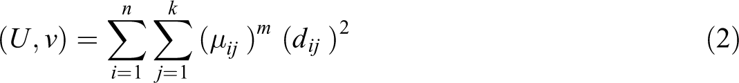
The optimal fuzzy partition of the data is the one that minimizes the objective function $j_{m}$ equal to the weighted sum of the quadratic distances between the observations and the centroids of each cluster

(U, v) = \sum_{i = 1}^{n} \sum_{j = 1}^{k} {(μ_{i j})}^{m} {(d_{i j})}^{2}

where m is the fuzzy weighting coefficient (1 ≤ m < ∞), whose function is to control the degree of overlap established between the clusters, and (d_ij)² is the square of the distance in the space of the attributes between the point i and the centroid class j, which can be calculated as follows

{(d_{i j})}^{2} = {‖x_{i} - v_{j}‖}^{2} = {(x_{i} - v_{j})}^{⊺} A (x_{i} - v_{j})

where x_i is the i-th observation of the data matrix X, v_j is the centroid of cluster j, and A is the positive definite weights matrix (p × p) that induces norm for the internal product. Weighting matrix A defines a distance normalization procedure. The result represents the distance between two points or vectors in a linear vector space. Fridgen et al. (2004) propose taking A = I (identity matrix), only when the variables are statistically independent and present the same variance. The metric obtained is, therefore, the Euclidean distance between the i-th observation and the centroid. If the variances of the variables are different, the variables should be standardized by using a diagonal matrix (A = D) whose terms are precisely the variances of the variables under study or the previously standardized variables should be used. Finally, the third possibility is to take A = S (matrix of variances and covariances of X), with which the resulting metric is the Mahalanobis distance. This distance is used when the classification variables not only show different variances but also are correlated with each other. While the fuzzy k-means iterative algorithm always converges to a local minimum of J_m from a given initial U, a different randomization of U might generate a different local minimum (Bezdek, 1981; Xie and Beni, 1991).

The fuzzy k-means fuzzy algorithm uses an iterative process to obtain the pair (U, V) that optimizes the fuzzy partition of the X data. The structure of the algorithm (Bezdek, 1981) is shown below.

The number of groups or clusters, k, is chosen, with 2 ≤ k ≤ n.

The value of the fuzzy exponent m is fixed, with 1 < m < ∞.

An appropriate measure of similarity or distance d_ij is selected.

The value of the convergence criterion (completion) of the algorithm is selected.

The maximum number of iterations is selected, l_max.

The matrix U⁰ is initialized with random values and according to the restriction specified in equation (1).

In the successive iterations l = 1, 2, 3…, V^l (centroid matrix) is recalculated from U (l.1), using the following expression

v_{i, j} = \frac{\sum_{j = 1}^{n} {(u_{i j})}^{m} x_{j}}{\sum_{j = 1}^{n} {(u_{i j})}^{m}}

The minimization of equation (2) by the iterative method of Picard makes it possible to calculate (update) U^l from the updated matrix V^l according to

u_{i j} = {[\sum_{j = 1}^{k} {(\frac{d_{i j}}{d_{l j}})}^{2 / m - 1}]}^{- 1}, i = 1, \dots, n j = 1, \dots, k

The algorithm is interrupted when the maximum number of iterations (l_max) is reached, or when $‖U^{1} - U^{(l - 1)}‖ \leq ε$ ; otherwise, return to step 7.

The indexes are finally computed to validate the clusters.

To evaluate the classification achieved with a certain number of groups, there are different indices, such as the partition coefficient (CP) (or fuzziness performance index (FPI), Bezdek, 1981), the entropy index of the classification (or normalized classification entropy (NCE), Bezdek, 1981), the Xie–Beni (XB) index (Xie and Beni, 1991), and the Fukuyama–Sugeno (FS) index (Fukuyama and Sugeno, 1989), among others.

The CP measures the degree of separation or overlap (degree of fuzziness) between the groups formed. The less diffuse the partition, the better the classification. It is calculated as follows

CP (U) = \frac{\sum_{i = 1}^{n} \sum_{j = 1}^{k} u_{i j}^{2}}{n}

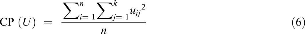
In this case, the optimum is given by maximizing CP and is equivalent to a classification, in which each observation belongs to a single cluster. The minimum is given when each observation belongs, with the same degree, to each cluster (greater uncertainty).

Partition entropy (EP) estimates the amount of disorganization created by the fuzzy partition of the data matrix X with a specific number of clusters. For this index, EP values close to 0 indicate a better classification, that is, with a higher degree of organization

EP (U) = \frac{\sum_{i = 1}^{n} \sum_{j = 1}^{k} u_{i j} log (u_{i j})}{n}

In the XB index, it is incorporated into V and X. This index prefers partitions whose intracluster distance is minimum and the intercluster distance is maximum

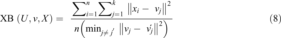
XB (U, v, X) = \frac{\sum_{i = 1}^{n} \sum_{j = 1}^{k} {‖x_{i} - v_{j}‖}^{2}}{n ({min}_{j \neq j^{'}} {‖v_{j} - v_{j} ´‖}^{2})}

The XB index is considered a measure of compaction within the cluster. A small value of XB represents a grouping where the groups are compact and well separated. Therefore, the best partition is obtained by minimizing XB.

The FS index is formed by the difference between the measure of compaction and the measure of separation between the centroids of the groups and the mean of all the centroids. The minimum of FS corresponds to a fuzzy partition with well-separated compact classes

FS (U, v, X) = \sum_{i = 1}^{n} \sum_{j = 1}^{k} u_{i j}^{m} ({‖x_{i} - v_{j}‖}^{2} - {‖v_{j} - \bar{v}‖}^{2})

It is important to consider that for a data set, the indexes may differ among them, that is, they may suggest different cluster numbers as optimal partition. One solution is to obtain a single index that summarizes the previous ones. In the mentioned indexes, except for the CP, a lower value of the index implies a better classification. Therefore, CP is recalculated as CP* = 1/CP so that the minimum value in all indices represents the best choice. Additionally, the index values are normalized between 0 and 1, by dividing each value by the maximum reached by the index in the different classifications. Then, the Euclidean distance for each classification is calculated using the values of the normalized indices and the lowest value classification of this new index is selected (Córdoba et al., 2013).

The indices provide information on the possible optimal classification. The final selection of the number of clusters must follow a compromise relationship between what is suggested by the indices and the economic criteria.

Classification of departments by fuzzy k-means clustering

Following Córdoba et al. (2012), the proposal for the delimitation of areas is based on the MULTISPATI-PCA and fuzzy k-means cluster analyses (Bezdek, 1981; Dray et al., 2008; Fridgen et al., 2004). In addition to the recorded variables, the database must include the spatial coordinates of each data point. Geographical coordinates are generally converted to Cartesian coordinates. This allows distances to be displayed as absolute (meters) instead of relative distances (degrees). The preprocessing stage can be performed using any geographic information systems. The next step in the algorithm is to apply MULTISPATI-PCA to tourism industries (H, ST, SC, AV, SD, R, and SV) and obtain the sPCs. The analysis can be performed with the “ade4” packages (MULTISPATI function, Chessel et al., 2004) and “spdep” (Bivand et al., 2014) of the R software (R CoreTeam, 2017). In this case, a binary matrix is defined, where two departments are considered neighbors if they have a common edge.

The function used to create the connection network was poly2nb from the “spdep” package. Using the “ade4” package (Chessel et al., 2004), the R software returns a MULTISPATI class object, which contains several elements, including the sPCs. A small set of these resulting synthetic variables, which account for a large amount of the total variation (≥70%), are subsequently used as input to the fuzzy k-means cluster analysis.

Finally, the fuzzy k-means cluster analysis is applied using the sPCs as variables on which the classification is based. Thus, the data matrix used in the fuzzy k-means analysis includes the n observations each with a <p sPCs. The Euclidean distance is used as a measure of similarity in the fuzzy k-means optimization function, since the main components are independent and standardized when the MULTISPATI-PCA is performed; therefore, their variances do not differ. The fuzzy exponent is set at the conventional value of 1.30 (Odeh et al., 1992). Alternatively, the fuzzy k-means algorithm can be implemented from another software tool, such as FuzMe (Minasny and McBratney, 2002), which, besides working with the Euclidean distance, allows the use of the Mahalanobis or diagonal distances, which are appropriate when the variables are not statistically independent and/or present different variances. The CP (also known as the FPI) and the NCE (Odeh et al., 1992) can be used to determine the optimal number of clusters. This is obtained when both indexes are reduced to a minimum, which represents the least overlap between groups (FPI) or the highest degree of organization (NCE) as a consequence of the data grouping process (Fridgen et al., 2004). To execute the new algorithm called fuzzy k-means cluster analysis on spatial main components, the scripts developed by Córdoba et al. (2012) in the R software are used with necessary adaptations to incorporate the activities at the departmental level (R CoreTeam, 2017).

Results and discussion

Spatial weighting matrix

To define the spatial weighting matrix, we considered a binary matrix. The simplest specification of a neighborhood is a connectivity matrix C, where c_ij = 1 if the spatial units i and j are neighbors, and c_ij = 0, two departments are considered neighbors if they have an edge in common. The function used to create the connection network was poly2nb from the “spdep” library (Bivand et al., 2017). The nb2listw function of the R software was used to determine the neighboring sites of each site. The spatial weight matrix was obtained after standardizing by row (style = W). The connection network is presented in Figure 3. The department with the largest number of neighboring was Santa María (nine links), whereas the departments with the fewest neighboring included Capital (two links), General Roca (two links), Minas (two links), Río Seco (two links), and Sobremonte (two links). On average, there were five neighboring sites at each point.

Figure 3.

Connection network.

Application of PCA and sPCA

The results (Tables 1 and 2) show that a lower proportion of the variance accumulated in the first two PCs is explained using MULTISPATI-PCA than using PCA (2.643 vs. 2.903 for axis 1 and 1.258 vs. 1.876 for axis 2).

Table 1.

Eigenvalues, spatial variance, and Moran’s index of the principal components generated by MULTISPATI-PCA (from the average share of activities).

Axis	Eigenvalues	Spatial variance	Proportion (spatial variance)	Accumulated proportion	Moran’s index
1	1.436	2.643	0.378	0.378	0.543
2	0.539	1.258	0.180	0.557	0.429
3	0.105	1.282	0.183	0.740	0.082
4	0.005	0.094	0.013	0.754	0.055
5	−0.013	0.252	0.036	0.790	−0.051
6	−0.106	0.452	0.065	0.854	−0.236
7	−0.186	1.019	0.146	1.000	−0.183

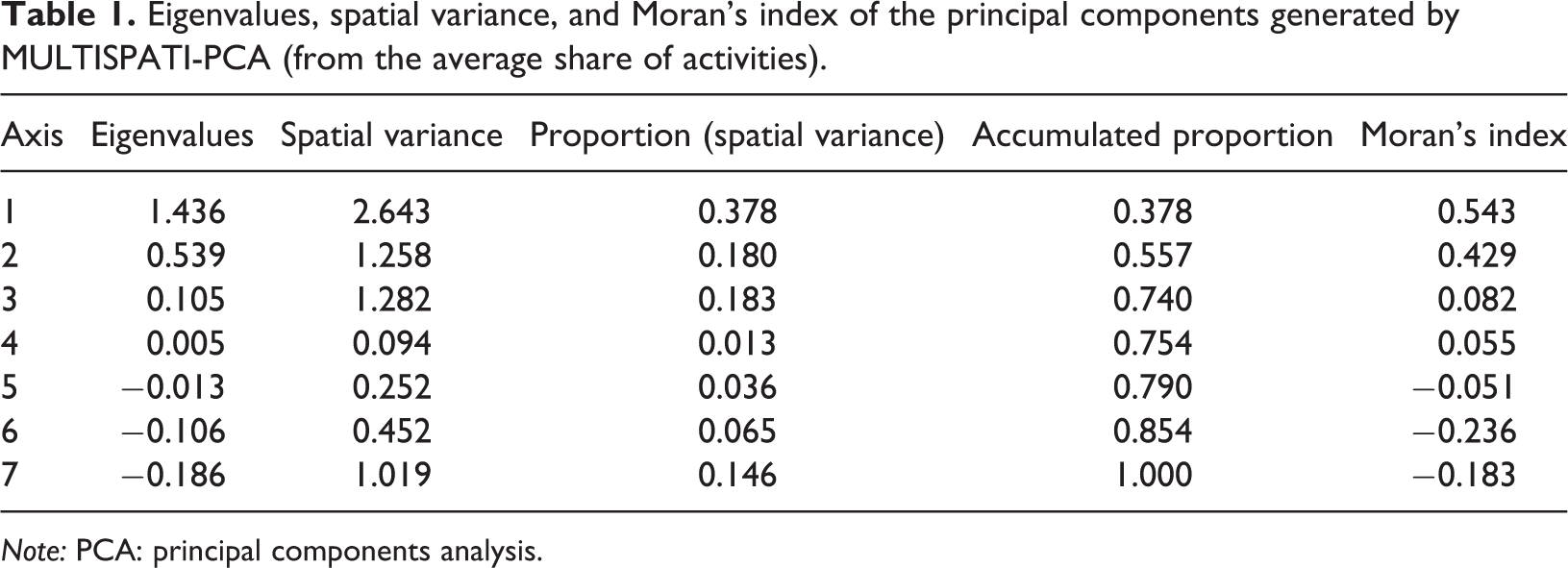
Note: PCA: principal components analysis.

Table 2.

Eigenvalues, spatial variance, and Moran’s index of the principal components generated by PCA (from the average share of activities).

Axis	Eigenvalues	Proportion	Accumulated proportion	Moran’s index
1	2.903	0.415	0.415	0.436
2	1.876	0.268	0.683	0.087
3	1.025	0.146	0.829	0.384
4	0.719	0.103	0.932	0.013
5	0.343	0.049	0.981	−0.161
6	0.118	0.017	0.998	0.046
7	0.016	0.002	1.000	−0.041

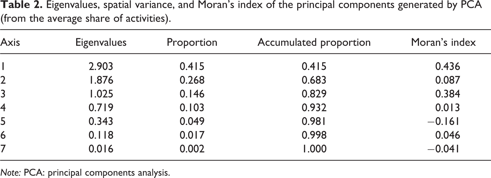
Note: PCA: principal components analysis.

Nevertheless, the MI values calculated for the first two PCs suggest that the estimation of autocorrelation increased with MULTISPATI-PCA with respect to that of PCA PCs (0.543 vs. 0.436 for axis 1; 0.429 vs. 0.087 for axis 2). This result suggests a better visualization of spatial variability using the spatially restricted analysis. By contrast, PC3 showed an inverse behavior. Therefore, it can be concluded that variance is not always reduced due to the estimation of autocorrelation, and that maximization of spatial variability depends on the characteristics of the present autocorrelation.

Figure 4 shows the first two components of PCA (left) and of MULTISPATI-PCA (right), as well as the eigenvalues associated with each of the axes (bar graph). Black bars correspond to the number of selected axes that were used to represent graphically and interpret the underlying variability, in this case, of the first two PCs. Black bars along with white bars indicate the number of axes obtained in the analysis. The height of each bar represents the proportion of total variability explained by each PC. Thus, for MULTISPATI-PCA, the first two PCs contribute sufficient information for the analysis, since the subsequent PCs do not make an important contribution (white bars).

Figure 4.

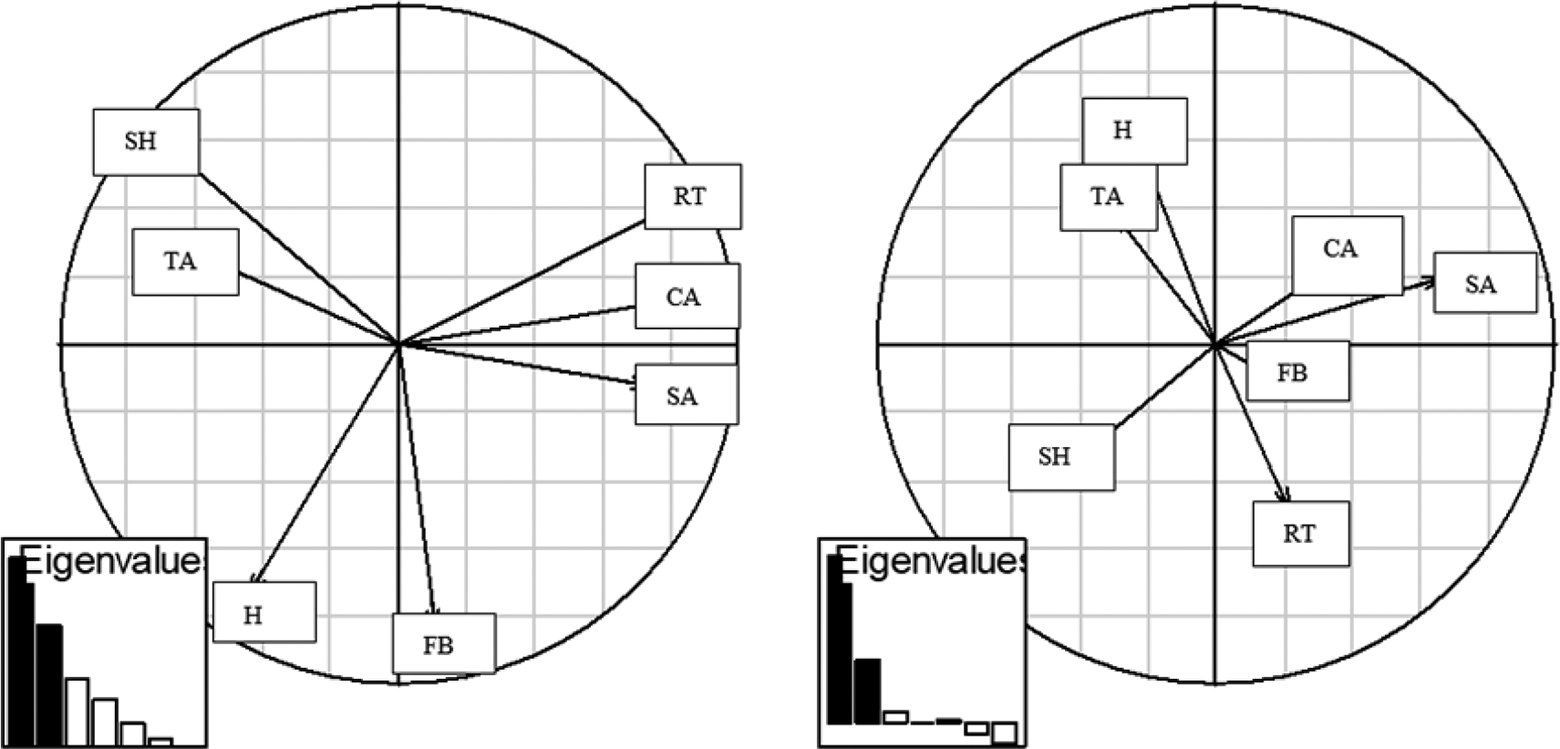
Graphical representation of the first two axes of PCA (left) and MULTISPATI-PCA (right), showing the correlation among variables and between variables and the principal components.

The variation in axis 1, for both methods, was strongly driven by CA and SA, the variable of greatest projection along the x-axis. However, differences between analyses were observed at the level of the co-variation structure between the two measurements of RT.

The relationships between CA and SA did not vary significantly, and correlations between H and TA did show a strong variation. The relocation of FB on the first axis of MULTISPATI-PCA produced a change in the weighting of variables on sPC2 (y-axis), with TA becoming more correlated with H.

The correlation between TA and H was recovered by PCA to a lower extent, as shown by the angle between the two vectors of the variable, and was more noticeable with MULTISPATI-PCA.

The relocation of food services (FB) on the first axis of MULTISPATI-PCA produced a change in the weighting of variables on PC2 (x-axis), which made more correlated with H and TA; thus, variability can be analyzed from a different dimension.

Figures 5 and 6 show the maps achieved by assigning each of the georeferenced sites to the values of PCA PC1 and PC2 and MULTISPATI-PCA, respectively. The multivariate spatial variability maps obtained with the PC1 of both methods were similar. This result is attributed to the fact that in both analyses PC1 is highly positively correlated with CA and SA, and negatively with SH. On the other hand, the variation of the H is mainly represented in the maps built from the PCA PC2, whereas in the map obtained with the MULTISPATI-PCA sPC2, the variability is mainly due to the H (Figure 6) does it to a greater extent together with other activities such as TA and contrasts with those whose variation is linked to transport services (RT); the black squares here represent values of higher H than the white squares as evidenced by the correlation structure of the variables (Figure 6).

Figure 5.

Maps of multivariate spatial variability from the PC1 of PCA (left) and PC2 of PCA (right).

Figure 6.

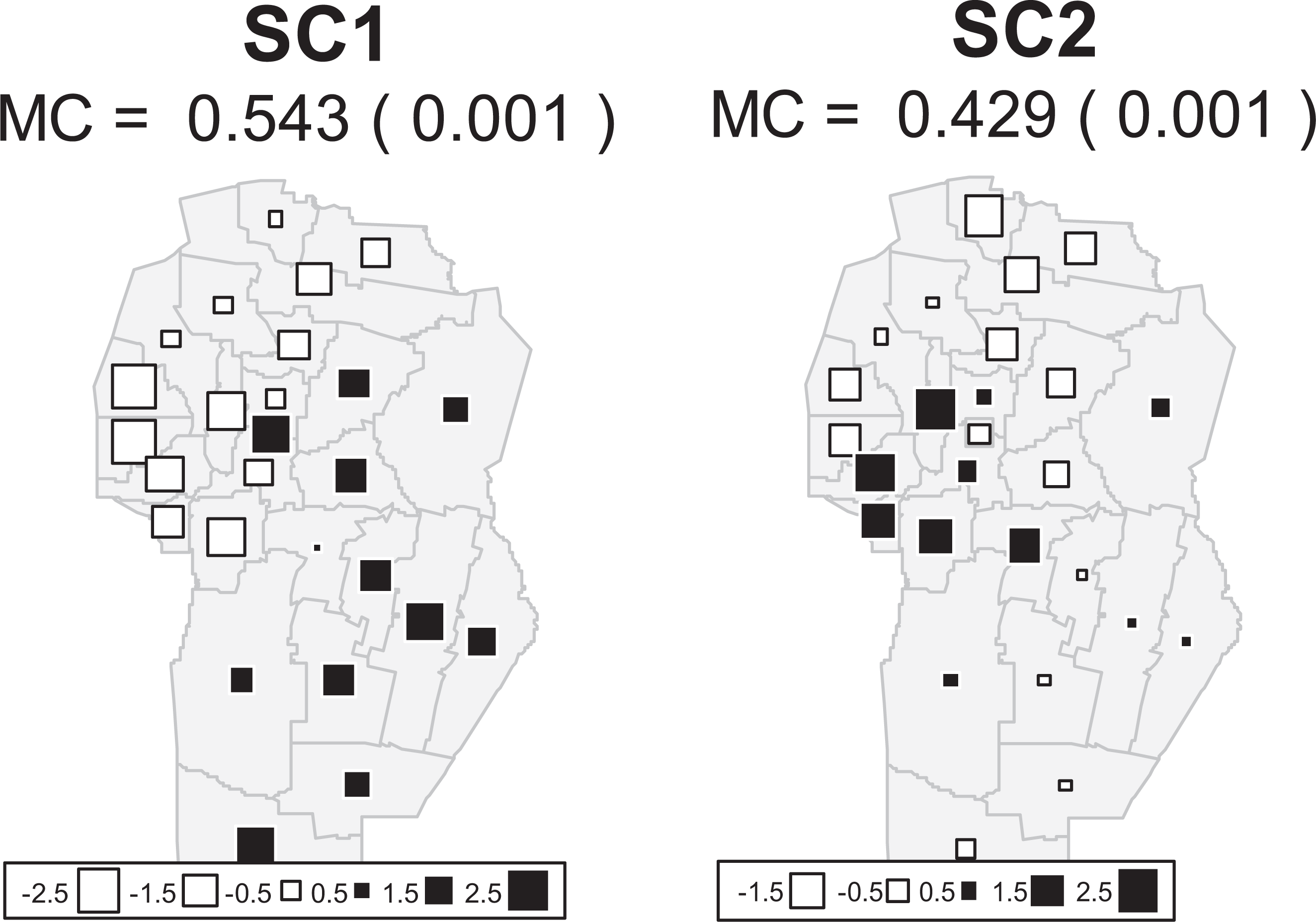
Maps of multivariate spatial variability from the PC1 of MULTISPATI-PCA (left) and PC2 of MULTISPATI-PCA (right).

Classification of departments by fuzzy k-means clustering

The indices used for the selection of the optimum number of classes yielded different numbers of clusters to be retained (Table 3). The CP, which represents the smallest overlap among groups, and the Fukuyama–Sugeno’s index suggest that four classes are the optimal partition. For the entropy index, which had the greatest degree of organization as a consequence of the clustering of classification data, and the XB index, the optimal number of classes suggested is three. A summary index, which contains information of each of the previously calculated indices, indicated an optimal partition of three classes.

Table 3.

Selection of number of classes of department partition.

Index	Two classes	Three classes	Four classes
Partition coefficient	1.053	1.039	1.053
Partition entropy	0.090	0.058	0.106
Xie–Beni	0.013	0.004	0.012
Fukuyama–Sugeno	−50.531	−63.157	−95.585
Summary index	1.929	1.710	2.526

Note: For each index, the value in bold represents the optimum number of classes suggested as indicated by the best index.

Considering the economic structures underlying the tourism industry, four classes (Figure 7) reveal the particular characteristics of the departments and their similarities and contribute an additional element for the analysis of regional development.

Figure 7.

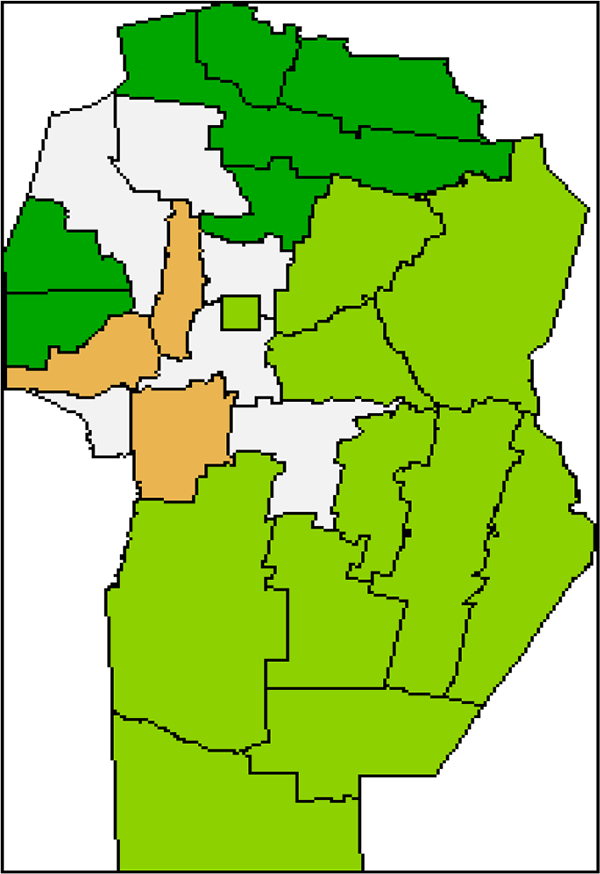
Cluster fuzzy k-means from MULTISPATI-PCA.

One area (class 1, light brown) is composed of Punilla, Calamuchita and San Alberto departments; another area (class 2, light green) includes departments from the southeast of the province and the Capital department; another area (class 3, white) includes San Javier, Ischilín, Cruz del Eje, Colón, and Santa María departments, and the last area (class 4, dark green) includes departments from the north (Sobremonte, Río Seco, Tulumba, and Totoral) and the west (Minas and Pocho) of the province. To give more information about the departments of Córdoba, Table 4 shows information on population and Figure 8 shows the natural areas of the province.

Table 4.

Departments of Córdoba.

Departments	Population	Male	Female	Hotel beds^a
Calamuchita	54,730	119,713	126,680	11,666
Capital	1,329,604	27,330	27,400	11,013
Colón	225,151	110,176	114,975	2262
Cruz del Eje	58,759	85,270	93,131	964
General Roca	35,645	26,006	27,514	153
General San Martín	127,454	62,417	65,037	1137
Ischilín	31,312	101,224	105,083	567
Juárez Celman	61,078	17,905	18,377	319
Marcos Juárez	104,205	50,972	53,233	842
Minas	4727	6496	6177	13
Pocho	5380	9319	9237	31
Presidente Roque Sáenz Peña	36,282	18,339	18,665	400
Punilla	178,401	18,041	17,604	36,520
Río Cuarto	246,393	634,341	695,263	2,553
Río Primero	46,675	6,710	6,532	155
Río Seco	13,242	2,378	2,213	102
Río Segundo	103,718	2,433	2,294	257
San Alberto	37,004	50,613	53,105	10,906
San Javier	53,520	23,230	23,445	1,065
San Justo	206,307	29,130	29,629	2,419
Santa María	98,188	2,769	2,611	1,198
Sobremonte	4,591	52,249	53,478	8
Tercero Arriba	109,554	15,159	16,153	883
Totoral	18,556	49,230	48,958	325
Tulumba	12,673	53,148	56,406	103
Unión	105,727	30,490	30,588	486
Total	3,308,876	1,605,088	1,703,788	86,347

Note: Sociodemographic characteristics and hotel beds.Source: Statistics and Census Agency of Córdoba, Córdoba Tourism Agency.

^a Hotel beds registered in the Córdoba Tourism Agency do not include the informal sector.

Figure 8.

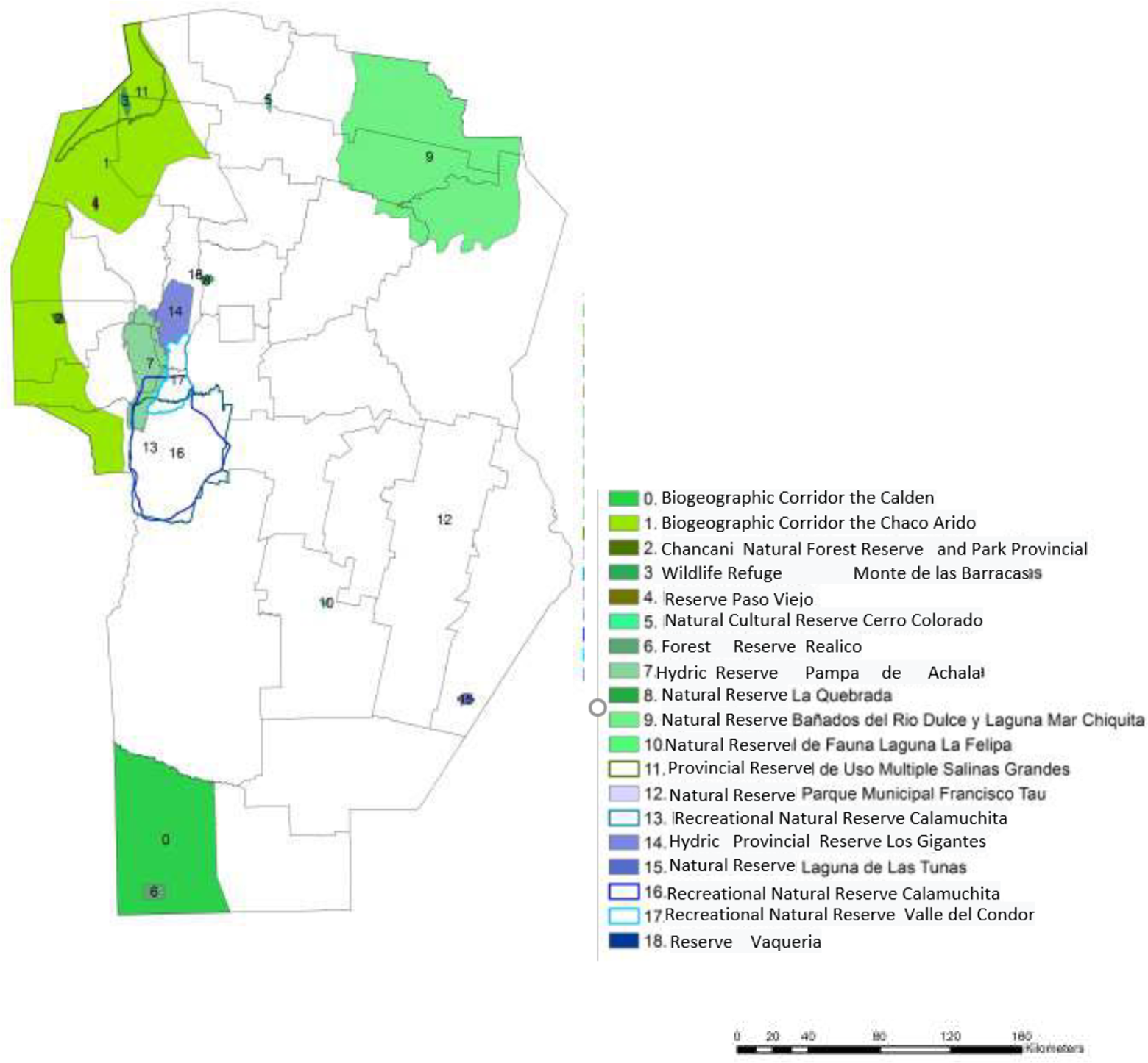
Natural areas of the province of Córdoba (2017). Maps: Córdoba Tourism Agency, Province of Córdoba.

Departments included in class 1 are characterized by the greatest tourism development, which is observed in both the demand (the region received the greatest number of tourists, 69.8%, in 2014/2015, as reported by the provincial government tourism agency), and the supply, since these departments have the greatest share of the value added of the tourism industries in the gross regional product (between 16.6% and 29.6%, Figure 8). In these departments, the accommodation offer has increased in the last years (especially cabins and other non-conventional accommodation); the same trend occurred in the gastronomic sector, which implies an impact on the generation of jobs in specific and complementary sectors. Job generation impacts directly on local economies. This area is characterized by the plurality of tourist attractions and resources based on nature and history. There are negative impacts due to the development of investments, non-compliance with current environmental legislation and other issues, which together lead to the degradation of resources. It is necessary to develop a plan to enhance some resources (accessibility, protection, conservation, and better management of information), to strengthen investments, especially in basic infrastructure (sewers and others), and to integrate the different localities.

Class 2 includes departments from the southeast of the province and the Capital department; these departments have structures related to the agricultural and industrial sectors, as well as important development of transport, CA and SA. The area has attractions with potential for development and current and future use, such as lagoons, watersheds, and natural environments; festivities and activities linked to identity are performed. Likewise, some aspects that hinder the tourist use of these resources are identified, such as the low state of conservation; the lack of signaling, facilities, and infrastructure (transport, telecommunications, and digital banking services); deficiencies in information and promotion (brochures); and the insufficient offer of tourist services, mainly recreational proposals. Actions are required to achieve a greater insertion of small agricultural producers in the tourist offer.

Class 3 includes departments with an important development of the service sector. The area has tourist circuits supported by the singularity of the landscape and its associated cultural manifestations. It offers a wide range of possibilities in terms of cultural tourism. There is an evident need for tourism ventures, improved gastronomic offer, and tourist information services.

Class 4 comprises Pocho, Minas, Río Seco, Sobremonte, Totoral, and Tulumba departments, which are poorer, with lower gross regional product. This region requires a strengthening of regional economies and their possible incorporation to the tourism activity by compatibility and complementarity. Many resources present in this area require their enhancement (legal protection, accessibility, signage, proposal of complementary activities, and others), such as regional productive activities (artisanal producers of honey, beer, wineries, olive trees, fruit and vegetables, and others). The same needs for enhancement are evident in the infrastructure and provision of general services (road network, communications, health, safety, and others) and the offer of tourist services (accommodation, gastronomy, and tourist information), which need to be strengthened in quantity and quality to improve competitiveness (controls, accommodation categorization, and professionalization of the sector).

Conclusions

In this work, tourism industries were analyzed using multivariate techniques with the aim of identifying the differences in economic structures of the provincial departments.

The multivariate technique, MULTISPATI-PCA, designed for exploring the relationships between variables and their spatial structure (autocorrelation), was appropriate for visualizing and exploring data of several regionalized variables at the same time. In the comparison of MULTISPATI-PCA versus PCA, using the spatially restricted analysis, the selection of the number of PCs for the interpretation of variability was nonambiguous. The degree of spatial structuring was greater with MULTISPATI-PCA than with not spatially restricted PCA. This was evident in the maps of synthetic variables, where the spatial structure was clearer when sPCs of MULTISPAI-PCA were used.

Considering the spatial dimension in the economic analysis may help improve interpretability of results. Spatial variability generates correlations between observations of a single variable that is repeatedly recorded in space and, therefore, data cannot be treated as statistically independent. Multivariate techniques facilitate the interpretation of complex relationships among variables, reduce dimension of the data set in order to map spatial variability, allow detection of structures, and reveal new spatial relationships that may not be evident when economic variables are analyzed individually.

The application of the fuzzy k-means clustering analysis including one spatial dimension through the use of spatial component analysis (MULTISPATI-PCA) showed that the classification into four department clusters is appropriate. Four classes reflect the particular characteristics of departments and their similarities considering the economic structures underlying the tourism industry. This stratification provides an additional element for analysis for the regionalization of tourism areas. This result is important because the provincial government is analyzing different zoning alternatives for the implementation of tourism development policies.

The use of these novel multidimensional mapping techniques provides a tool to address new analysis dimensions, contributing with insights to different alternatives for regional development.

The results of this study may generate different lines of research to address some of the weaknesses and questions. Firstly, it would be interesting to test if the same results are obtained by applying other neighborhood criteria. Secondly, other variables may be incorporated to the analysis to obtain information that would substantially enrich the present results. Finally, the evolution of the identified patterns over time should be studied.

Footnotes

Declaration of conflicting interests

The author(s) declared no potential conflicts of interest with respect to the research, authorship, and/or publication of this article.

Funding

The author(s) received no financial support for the research, authorship, and/or publication of this article.

ORCID iD

Laura I Luna

References

Anselin

Florax

(1995) New directions in spatial econometrics. In: Anselin

Florax

(eds) New Directions in Spatial Econometrics. Berlin: Springer, pp. 3–18.

Arrouays

Saby

Thioulouse

, et al. (2011) Large trends in French topsoil characteristics are revealed by spatially constrained multivariate analysis. Geoderma 161: 107–114.

Bezdek

(1981) Objective function clustering. In: Pattern Recognition with Fuzzy Objective Function Algorithms. Advanced Applications in Pattern Recognition. Boston, MA: Springer, pp. 43–93.

Bivand

(2008) Implementing representations of space in economic geography. Journal of Regional Science 48: 1–27.

Bivand

(2014) Creating neighbours. Available at: https://cran.r-project.org/web/packages/spdep (accessed 25 January 2017).

Bivand

Altman

Anselin

, et al. (2017) Spdep: spatial dependence: weighting schemes, statistics and models. R package version 0.5-56. Available at: https://cran.r-project.org/web/packages/spdep (accessed 25 January 2017).

Capone

Boix

(2008) Sources of growth and competitiveness of local tourist production systems: an application to Italy (1991–2001). The Annals of Regional Science 42: 209–224.

Chessel

Dufour

Thioulouse

(2004) The ade4 package-I-One-table methods. R News 4: 5–10.

Chhetri

Arrowsmith

Chhetri

, et al. (2013) Mapping spatial tourism and hospitality employment clusters: An application of spatial autocorrelation. Tourism Analysis 18: 559–573.

10.

Cliff

Ord

(1973) Spatial Autocorrelation. London, UK: Pion Limited.

11.

Córdoba

Balzarini

Bruno

, et al. (2012) Identificación de zonas de manejo sitio-específico a partir de la combinación de variables de suelo. Ciencia y Tecnología Agropecuaria 13(1): 47–54.

12.

Córdoba

Bruno

Costa

, et al. (2013) Subfield management class delineation using cluster analysis from spatial principal components of soil variables. Computers and Electronics in Agriculture 97: 6–14.

13.

Córdoba Tourism Agency (2019) Plan Estratégico de Turismo Sostenible 2030. Agencia Córdoba Turismo Gobierno de la Provincia de Córdoba. Available at: https://www.cordobaturismo.gov.ar/plan-estrategico-de-turismo-sustentable (accessed 10 January 2020).

14.

Dray

Chessel

Thioulouse

(2003) Co-inertia analysis and the linking of ecological data tables. Ecology 84(11): 3078–3089.

15.

Dray

Saïd

Débias

(2008) Spatial ordination of vegetation data using a generalization of Wartenberg’s multivariate spatial correlation. Journal of Vegetation Science 19(1): 45–56.

16.

Fridgen

Kitchen

Sudduth

, et al. (2004) Management zone analyst (MZA): software for subfield management zone delineation. Agronomy Journal 96: 100–108.

17.

Fukuyama

Sugeno

(1989) A new method of choosing the number of clusters for the fuzzy c-means method . In: Proceedings of the Fifth Fuzzy Systems Symposium, pp. 247–250 (in japanese).

18.

Gabriel

(1971) The biplot graphic display of matrices with application to principal component analysis. Biometrika 58(3): 453–467.

19.

Gabriel

Sokal

(1969) A new statistical approach to geographic variation analysis. Systematic Biology 18(3): 259–278.

20.

Geary

(1954) The contiguity ratio and statistical mapping. The Incorporated Statistician 5(3): 115–146.

21.

Gooroochurn

Hanley

(2005) Spillover effects in long-haul visitors between two regions. Regional Studies 39(6): 727–738.

22.

Hall

(2005) Tourism: rethinking the Social Science of Mobility. Harlow, UK: Pearson Education.

23.

Instituto Nacional de Estadística y Censos (INDEC) (2010) Censo Nacional de población, hogares y viviendas 2010. Available at: https://www.indec.gob.ar/indec/web/Nivel4-Tema-2-41-135 (accessed 25 January 2018).

24.

Instituto Nacional de Estadística y Censos (INDEC) (2018) Encuesta de Ocupación hotelera (EOH). Available at: https://www.indec.gob.ar/indec/web/Nivel4-Tema-3-13-56 (accessed 25 January 2019).

25.

Krugman

(1998) What’s new about the new economic geography? Oxford Review of Economic Policy 14(2): 7–17.

26.

Lazzeretti

Capone

(2009) Spatial spillovers and employment dynamics in local tourist systems in Italy (1991–2001). European Planning Studies 17(11): 1665–1683.

27.

Lee

Schachter

(1980) Two algorithms for constructing a Delaunay triangulation. International Journal of Computer and Information Sciences 9: 219–242.

28.

Minasny

McBratney

(2002) FuzME Version 3.0. Australian Centre for Precision Agriculture. The University of Sydney. Available at: http://www.usyd.edu.au/su/agric/acpa (accessed 10 June 2017).

29.

MINTUR (2012) Anuario Estadístico de Turismo 2012 Buenos Aires, Argentina, Ministerio de Turismo de la Nación. Available at: https://www.yvera.tur.ar/estadistica (accessed 15 March 2018).

30.

Moran

(1948) The interpretation of statistical maps. Journal of the Royal Statistical Society 10: 243–251.

31.

Neumayer

(2004) The impact of political violence on tourism: dynamic cross-national estimation. Journal of Conflict Resolution 48(2): 259–281.

32.

Odeh

IOA

McBratney

Chittleborough

(1992) Soil pattern recognition with fuzzy-c-means: application to classification and soil-landform interrelationships. Soil Science Society of America Journal 56: 505–516.

33.

Pearson

(1901) LIII. On lines and planes of closest fit to systems of points in space. The London, Edinburgh, and Dublin Philosophical Magazine and Journal of Science 2(11): 559–572.

34.

R Core Team (2017) R: a language and environment for statistical computing R Foundation for Statistical Computing, Vienna, Austria. Available at: https://wwwR-projectorg/ (accessed 27 June 2018).

35.

Rodríguez Rangel

Sánchez Rivero

Ramajo Hernández

(2020) A spatial analysis of intensity in tourism accommodation: an application for Extremadura. Economies 8(2): 28.

36.

Saby

NPA

Thioulouse

Jolivet

, et al. (2009) Multivariate analysis of the spatial patterns of 8 trace elements using the French soil monitoring network data. Science of the Total Environment 407: 5644–5652.

37.

United Nations and World Tourism Organization (UNWTO) (2010), International Recommendations for Tourism Statistics 2008 (IRTS 2008), (New York, Madrid, 2008).

38.

Xie

Beni

(1991) A validity measure for fuzzy clustering. IEEE Transactions on Pattern Analysis and Machine Intelligence 13(8): 841–847.

39.

Yang

Fik

(2014) Spatial effects in regional tourism growth. Annals of Tourism Research 46: 144–162.

40.

Yang

Wong

(2013) Spatial distribution of tourist flows to China’s cities. Tourism Geographies 15(2): 338–363.