




Abstract
Most prior work on educational homogamy does not distinguish between college attendees who marry someone who attended the same university (same-university marriages) and those who marry someone who attended a different university (different-university marriages). This article estimates the prevalence of partnering between individuals who attended the same university in the United States. Using rich data from the Panel Study of Income Dynamics (PSID), this study finds that, among college graduates who marry other college graduates, about one third have same-university spouses. As higher education has massified and feminized, rates of same-university marriages have changed very little between 1973 and 2013. By distinguishing between same-university and different-university marriages, this article highlights the role that universities, as organizational settings, play in structuring elective affinities – Pierre Bourdieu’s term for the class-based shared experiences and tastes that form the basis of social and romantic ties. Educational homogamy contributes to social stratification by consolidating the educational and social advantages of the individuals and same-university marriages make up a significant portion of these partnerships.
Introduction
Educational homogamy (marriages between individuals with the same level of education) contributes to social stratification in the United States (Kalmijn, 1998; Blossfeld and Timm, 2003). When highly educated individuals marry, they consolidate their social and economic advantages in a single family, securing the well-being of the individuals and providing resources that allow their children to thrive (Kalmijn, 1998; Mare, 1991). The flip side to this process is the exclusion of those with less education whose marriages do not bring together as many resources or who are less likely to marry at all (Edin and Reed, 2005; Wilcox and Wolfinger, 2007). While universities advertise the labor market outcomes of their graduates, there is a growing sense that they also confer additional benefits: a university degree allows graduates to access advantageous positioning in marriage markets. In this way, educational homogamy, marriages between individuals with the same level of education, contributes to the reproduction of social stratification in the United States.
Description of the contribution of this study
Most prior work on educational homogamy does not distinguish between college attendees who marry someone who attended the same university (same-university marriages) and those who marry someone who attended a different university (different-university marriages). However, distinguishing between these two types of marriages allows researchers to better understand (1) the mechanism underlying educational homogamy and (2) the role of universities as organizations in marital formation. Among college attendees, are most of these educationally homogamous marriages between people who went to the same university? This would suggest that educational homogamy is driven by individuals meeting during their college years. Conversely, are most educationally homogamous marriages among people who attended different institutions? A finding in this direction would suggest that university credentials are associated with educational homogamy through individuals’ post-college sorting of potential spouses. Untangling these two types of educational homogamy (same-university vs different-university) allows us to see more clearly the role universities play in educational matching. Understanding the role universities play in marital formation is a vital piece of the puzzle to understanding educational homogamy overall.
This study investigates the rates of marriage between individuals who attended the same institutions, characteristics of institutions (such as gender ratio, size, and selectivity) associated with university-level educational homogamy, and how these patterns have changed over time. The study aims to answer the following research questions:
What is the rate of same-university educational homogamy in the United States?
Has the rate of same-university educational homogamy changed over time?
Data from the Panel Study of Income Dynamics (PSID) are analyzed by estimating a series of logistic regressions. The author finds that among university attendees who marry other university goers, about one third attended the exact same institution as their spouses. This figure has fluctuated very little between cohorts of 25- and 34-year-olds over the last five decades and indicates that universities are playing a significant role in American marital formation. The author also finds that some university-level institutional characteristics, such as affiliation and gender ratio, are associated with marrying someone who attended the same university. For example, people were most likely to partner with others on campus when they attended public institutions with balanced gender ratios. These findings suggest that college attendance – and more specifically the institution attended – plays a role in structuring marital outcomes. Demographers have long understood that couples often share the same education level (Mare, 1991; Kalmijn, 1998). However, this article demonstrates that what is shared within marriages is more than just education level; often for college attendees, it is the exact same higher educational institution.
The following section describes how educational homogamy is a piece of the larger puzzle of social reproduction (of which education is a central engine). The next section discusses the extant empirical research on marriages between people with similar levels of education (educational homogamy) and the resulting distribution of social and economic resources. The article then proceeds to present data and analytic strategy, followed by findings and discussion.
Theoretical framing: education and social reproduction
This article aims to add to the literature the role of education in social reproduction. In the following section, I examine the theories that link education to processes of social reproduction. These ideas, rooted in Marxist and Bourdieusian traditions, focus on classroom practices, curricula (the hidden curriculum), and interactions with teachers in primary and secondary schools. In this theoretical tradition, types of occupations are the main outcome – for example, does a student become a worker, manager, or a professional? However, there is an additional, often overlooked set of outcomes that are a direct result of education’s role in social reproduction: educationally homogamous marriages. I review literature that indicates how educational homogamy contributes to social stratification. The goal here is to demonstrate in the empirical literature that the powerful role education plays in social reproduction is not limited to just the occupational outcomes, it functions through the marital outcomes of graduates as well.
The hidden curriculum and social reproduction
Bowles and Gintis (1976), Marxist reproduction theorists, wrote extensively about the ways that schooling reproduces and legitimates social inequality by ensuring that social origins determine social destinations. In their classic text, Bowles and Gintis (1976) argue that the education system is merely an extension of the capitalist labor market. To function, capitalism needs masses of workers and a relatively small number of bosses. To meet this need, two disparate school systems are maintained: one for educating working-class children who will be tomorrow’s workers and one for educating upper-class children who will be tomorrow’s bosses (Anyon, 1981). Working-class schools reward punctuality, direction following, and the completion of rote tasks – all good skills for disciplining the future worker (Ferguson, 2017). In contrast, upper-class schools encourage individuality and reward thinking outside of the box (Anyon, 1980). In each of these school types, students experience instruction that corresponds with their expected occupational destination, which corresponds with their social origins. Schooling legitimates existing inequalities by awarding failing grades to working-class children and validating upper-class children’s feelings of superiority and entitlement with high marks (Anyon, 1980; Bowles, 1977; Bowles and Gintis, 1976; Bowles and Gintis, 2002).
Early scholarship on education’s role in social reproduction focused on the question of, ‘How do schools produce workers and bosses?’ (Bhattacharya, 2017). Bourdieu and Passeron’s (1979) theorizing differed in that they did not think that schools produced anything. Rather, working-class and upper-class home cultures created students (Bourdieu and Passeron, 1979 [1964]). Upper-class students experience a match between their bourgeois home ways, rules, and values and those of the school setting. This leads to classrooms where upper-class students feel a sense of belonging and working-class students have a pervasive sense of being out of place. These feelings of ease and unease contribute to differential educational achievement. In this way, for upper-class students, schools ‘transmute privilege into merit’ (Bourdieu and Passeron, 1979 (1964): 68).
Bourdieu’s ‘elective affinities’
While Bourdieu never posited a formal theory of educational homogamy, the notion of ‘elective affinities’ suggests that unions form between people who hold similar social/cultural positions and lifestyles and inhabit the same social space (Nagel et al., 2011; Schmitz, 2012). Elective affinities, ‘represented by all acts of co-option in fellow-feeling, friendship or love . . . lead to lasting relations . . .’ (Bourdieu, 1984: 241). Researchers have tested whether ‘elective affinities’ are shared within couples and have found that in fact couples have homogeneous tastes and often meet in a shared social space (Silva and Roux, 2011). The higher education system, which selects students mainly from the dominant classes, facilitates social reproduction via elective affinities (Bourdieu, 1984).
By the time young adults reach university, their cultural tastes and preferences for food, entertainment, and sports may match with that of their peers. These peers, who may be potential marital partners, may also feel an affinity toward one another or affiliation to the university based on social and cultural preferences that are affirmed by school experiences. Connections through university-based co-curricular activities may also build the kind of social capital connections that would give rise to future relationships (Coleman, 1988; Putnam, 2000). Given that marriages, especially marriages between educationally advantaged individuals, consolidate resources within a family, the institutions that structure these relationships are implicated in the reproduction of inequality.
Relevant literature
Educational homogamy
In the United States, marriages between individuals with the same level of education have become more common in the last 40 years (Mare, 2016). This trend is particularly strong among those with the highest levels of academic attainment, with the most divisive educational boundary existing between 4-year college graduates and individuals with fewer years of schooling (Breen and Salazar, 2011; DiMaggio and Mohr, 1985; Kalmijn, 1998; Mare, 1991). In recent decades, individual reports of valued characteristics in an ideal spouse shifted (Bottero and Prandy, 2001). In the 1930s, education was ranked 11th out of 18 desired spousal qualities (Boxer et al., 2015). Today, respondents rank education as the fourth most important spousal quality, following ‘mutual love and attraction’, ‘dependable character’, and ‘emotional stability’ (Boxer et al., 2015). In 2005, more than 55% of marriages in the United States were between people with the same level of education; the figure for college graduates was slightly higher than those with less than college education (Schwartz and Mare, 2005). In addition, there are indications that among college graduates, individuals have historically married others who attended colleges with similar characteristics (Arum et al., 2008). Observed rates of educational homogamy exceeded estimated rates under random marriage in France, the Netherlands, Italy, Spain, Great Britain, Denmark, Sweden, Hungary, Slovenia, the United States, and Germany (Blossfeld and Timm, 2003). Similar patterns have been found in the former Soviet Union (Gerber and Schwartz, 2009) and in Mexico, Chile, and Brazil (Torche, 2011). In addition, an important study of marriages in Denmark, Sweden, and Switzerland took up the main questions of this article – how much educational homogamy occurs between people who attended the same institutions and how much is the function of people partnering with others who attended different institutions. Nielsen and Svarer (2009) found that much of the systematic sorting of marriages by education is due to marriages between people who attended the same university or nearby university.
Families and social stratification
While understanding the marital patterns of college attendees is an interesting outcome in and of itself, it is also indicative of the consolidation of social advantages among an already advantaged group (college attendees), which has implications for patterns of resource distribution and social stratification between families (Breen and Salazar, 2011; Kalmijn, 1998; Mare, 1991). Even with the massification of higher education that occurred in the United States in the last 40 years, the advantages conferred by a university degree have not diminished. Students from all backgrounds receive the benefits of having a bachelor’s degree credential in the labor market. Despite this dramatic increase in higher education attendance, students whose parents went to college are still more likely to attend and graduate college themselves (Taylor and Cantwell, 2018). Some media reports suggest that students from high-income families are more likely than their low-income peers to marry a college classmate (Carey, 2018). In this way, despite some ways that universities have opened access to less advantaged populations, in others, higher education reproduces existing patterns of social stratification.
Dramatic changes in family structure between levels of educational attainment have also contributed to income inequality. While 90% of Americans marry at least once, college-educated individuals are the most likely to marry and stay married (Cherlin, 2010). Family structure drives income inequality because economic and social resources are pooled if more than one adult is present in the family unit. College graduates most often marry other graduates (Schwartz and Mare, 2005), and the correlation between spouses’ incomes has strengthened over time (Burtless, 1999). While college graduates are consolidating their wealth, non-college graduates are consolidating disadvantage. Female non-graduates are likely to marry other non-graduates and are the group most likely to be single parents (Martin, 2006). The following section describes the data and analytic strategy.
Data and methods
The data used for this study come from three sources: (1) individual characteristics for each spouse from the PSID publicly available data set; (2) PSID restricted-use data, which the author collected and recorded from archived questionnaire responses in the PSID repository and coded with institutional identifiers, including the universities respondents and their spouses attended; and (3) institutional characteristics of the universities from the National Center for Education Statistics’ (NCES) Integrated Postsecondary Education Data System (IPEDS) data sets. The PSID is a longitudinal study of a nationally representative sample of American individuals and their families. Housed at the University of Michigan’s Survey Research Center and funded by the National Science Foundation, the PSID follows the same individuals and families longitudinally, surveying them every 2 years. The survey focuses on economic, educational, and health indicators. The survey has followed the same American families from the first data collection in 1968 to today. The PSID main study is an excellent resource for examining White Americans and Black Americans. In 1968, when the survey selected the families, it would sample and follow longitudinally, large waves of immigration from Latin America, Asia, and other nations that had not started. A sample that was primarily comprised of White and Black Americans was representative of the United States. Despite efforts to add other racial groups to the survey in the 1990s, the PSID has not sufficiently gathered data from other racial groups (<3% of the sample is neither Black nor White). As a result of this historical oversight and data limitation, for this project, only African American and Caucasian individuals are included in the sample. An indicator variable for race (Black = 1; non-Black = 0) is included to test for the effects of race on educational homogamy. Given that Latinos and Asians are growing racial groups, it is regrettable that these data do not allow us to make inferences about the marital behavior of these groups. As a result of these limitations, race is accounted for in the model, but will not be a major focus of the analysis.
For this project, the PSID data set is restricted to include the first marriage of college attendee adults between 1975 and 2005. The period between 1975 and 2005 is examined because it spans the period of mass expansion and feminization of American higher education. Therefore, the sample includes individuals who attended college when men outnumbered women in higher education, individuals who were in college around the time of gender parity in 1982, and also college attendees who left college (and negotiated the marriage market) since women became the majority of college-goers. 1 For studying the US case, PSID is the best available data, as it is nationally representative and intergenerational. Similar studies in other countries have employed register data to examine these questions (e.g. Nielsen and Svarer, 2009). The author concedes that the study is limited by utilizing nationally representative survey data rather than register data.
Variable definitions and analytic strategy
In this study, marriages refer to the first marriage of individuals in the sample. No second marriages, such as a remarriage after divorce, are included in the sample. While this sample does not account for the variety of marital trajectories available to Americans, by isolating first marriages, this article offers conservative estimates of educational homogamy. Schwartz and Mare (2012) conclude that ‘despite the high prevalence of divorce, remarriage and continued schooling after marriage in the United States, the key to understanding trends in educational homogamy lies primarily in the variation in assortative mating into first marriage’ (Schwartz and Mare, 2012: 629). This is because prevailing marriages tend to be educationally homogamous, so estimates of homogamy among first marriage are conservative estimates of educational homogamy in the entire stock of marriages in a particular era (Schwartz and Mare, 2012).
The dependent variable for the analyses is the likelihood of having a spouse who attended the same university. A same-university spouse is defined as occurring when individuals and their spouses have an exact match of institutional code for any college they mentioned attending. Respondents could name up to two institutions that they attended. For example, some respondents mentioned a community college and then a university into which they transferred. Others mentioned a 4-year university and then another institution where they had done graduate work. PSID survey administrators recorded the most recent institution attended. In most cases, only one college name was listed for each spouse. When labeling a marriage as ‘same-university’, this article does not make distinctions about how couples met and married. Same-university couples could have started dating during their undergraduate years and married years later, they could have met through school alumni or friendship networks years later, or they may have met online or in some other fashion and coincidentally attended the same institution. All of these couplings are included under our measure of same-university marriage. However, in an analysis of the age difference among same-university spouses, the median age difference was 2 years; the mode was 1 year. Only 8% of same-university matches had an age difference of greater than 4 years. Although it is not possible to say with certainty that individuals knew each other on campus, the close proximity of ages suggests that campus friendship, acquaintanceship, or courtship was probable.
All individuals in the sample attended 4-year baccalaureate degree granting universities. IPEDS data sets do not contain information about the SAT scores of community college students because these institutions, which for the most part have open-admissions policies, do not collect or report their applicants’ scores. A small number of individuals who attended single-sex universities, defined as universities whose student bodies were comprised of over 90% one sex, were removed from the sample because they downwardly bias the results for same-university matching. Every person appears in the data only one time, at the moment of the inception of their first marriage, so this work compares the marital patterns of young adults when they were in young adulthood. For easier visualization of the descriptive results and to test for cohort effects in the multivariate analyses, the sample is divided into five cohorts, each comprised of 25- to 34-year-olds (Table 1).
Cohorts used for data analysis.
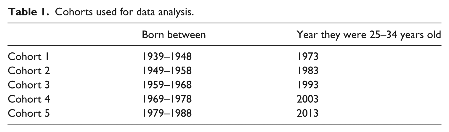
Cohort 1 was born between 1939 and 1948, so they were 25–34 years old in 1973. Cohort 2 was born between 1949 and 1958, so they were 25–34 years old in 1983. Cohort 3 was born between 1959 and 1968, so they were 25–34 years old in 1993. Cohort 4 was born between 1969 and 1978, so they were 25–34 years old in 2003. Finally, Cohort 5 was born between 1979 and 1988, so they were 25–34 years old in 2013. Another way to think about these groups would be to look at them in 2013: the 65- to 74-year-olds are Cohort 1, the 55- to 64-year-olds are Cohort 2, the 45- to 54-year-olds are Cohort 3, the 35- to 44-year-olds are Cohort 4, and the 25- to 34-year-olds are Cohort 5.
Baseline models control for several key variables. The demographic characteristics of the sample are controlled for using race (indicator variable for Black) and age when newlywed (a continuous variable of year the marriage occurred minus the year the individual was born). Since marriage markets for men and women are governed by different factors, all analyses are performed separately by gender. Two key socioeconomic variables are included in the model. A measure of family income at time of marriage accounts for multiple-earner families and non-labor income (such as stocks and other kinds of income more common in families of higher SES). The PSID measures the total income from all family members that includes all taxable labor market earnings and transfer income. This is a blunt measure of family economic position and status. However, taking an average of 5 years of family income prior to the year of marriage aims to smooth out of the year-to-year fluctuation in family earnings. While some might argue that the adults marrying in the sample, aged 24–35 years, are entirely independent of their families, the social status of their family of origin is unimportant. However, while most people in the mid-20s and 30s may indeed be financially independent of their families, it is likely that marital partners are aware of (and take into account as favorable or unfavorable) the family status of their potential partners (Charles et al., 2013). The purpose of including a variable for family income (along with a variable for parent education) is to account for some of the variation in family status. The economic and educational environment within which the person was reared is a marker of social status and likely picks up some of the unmeasured social and cultural capital. Parental educational attainment and an average of family income are entered models to account for family of origin socioeconomic status.
The college characteristics included in the models as independent variables each have theoretical significance. The number of women in higher education increased dramatically during the period studied and the gender ratio on individual campuses tipped toward women. Therefore, an independent variable for percentage of female students on campus is added. This variable was calculated by dividing the enrollment of women by total enrollment. Single-sex colleges were excluded from the analysis. College size and public/private status are variables that are speculated to have a relationship with marital choices, so these variables are added to our models to test these relationships. Barron’s categorical codes 1, 2, and 3 are used as a categorical measure of selectivity. Barron’s codes have emerged in the literature as the most efficient and common way to quantify selectivity (Eide et al., 2016; Ford and Thompson, 2016; Torche, 2011). Barron’s codes group institutions together based on a variety of institutional characteristics such as class rank, median test score, and percentage of students admitted. Following the lead of other researchers, ‘selective schools’ are coded using Barron’s ‘highly competitive’ or ‘most competitive’ categories (Eide et al., 1998; Torche, 2011) and omit institutions categorized as ‘special’, as these institutions largely base admissions decisions on non-academic criteria (Schmitz, 2012). Detailed descriptive statistics and discussion of variable coding are presented in Table 2.
Variables of interest: definitions, sources, and descriptive statistics.

SD: standard deviation; PSID: Panel Study of Income Dynamics; IPEDS: Integrated Postsecondary Education Data System.
For the logistic regression analyses, the sample is restricted to only college attendees whose spouses attended college. This sample specification allows for tests of characteristics associated with the likelihood of same-university marriages conditional on marrying someone who also attended university. The equation for the logistic regressions is

where π is the probability of marrying someone who attended the exact same university, S is a vector of individual characteristics (race, family income, highest parental education, cohort, and age when married), and P is a vector of institutional characteristics (selectivity, size, public/private, and gender ratio).
This study uses observational data to describe relationships and associations and does not make causal claims. 2 Multi-level modeling strategies are not used because of an interest in the effects of specific institutional characteristics rather than the effects of institutions as a whole. While individuals are nested in institutions, the author seeks to test the relationship between institutional characteristics (gender ratio and selectivity) and marital choices, not the effect of attending the South State University on marital choice. The aim of the analysis is to understand the institutional characteristics that create the conditions, on average, that are related to educational homogamy, not to isolate which institutions themselves are the major players in the educational homogamy landscape. Because to the nature of the PSID data set (organized by families), the standard errors have been clustered.
Findings
Overall, about 33% of married college attendees married someone who attended the exact same institution (Table 3). This rate of marriage formation varies very little between the first four cohorts of young adults, but increases substantially (and in the multivariate models statistically significantly) for the most recent cohort. For married college attendees aged 25–34 years in 2013, men married a same-university spouse 41% of the time, while women married a same-university spouse about 37% of the time. While women outpaced men in their rates of same-university marriages in 1973, men were entering into same-university marriages at higher rates than women by 2013.
University attendees married to university educated spouses 1973–2013 (by gender).
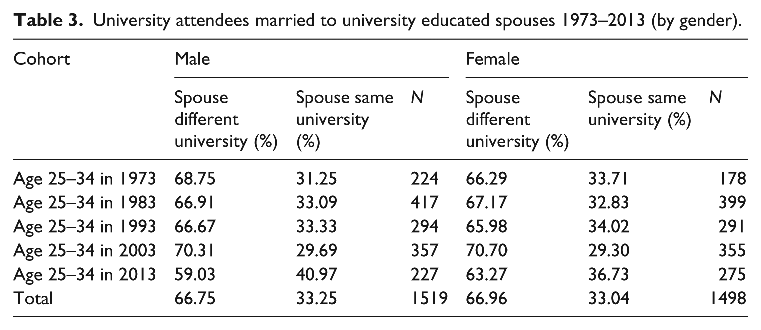
Some of the variation in same-university partnering across years can be explained by changes in patterns of marriage formation – that is, the stock of people who are marrying has changed over time. These patterns are explored more in Table 4, which provides detailed estimates of trends in individuals staying single and taking spouses who did not attend college. It is clear that young adults in the last cohort (25–34 in 2013) are delaying marriage formation, as 43% of them are single compared to 17% in 2003 and, most starkly, 3% in 1973. While this study finds that among married college attendees, the 2013 cohort had the largest rate of same-university marriages (41%), the cohort also had the lowest rate of individuals choosing into marriage.
Marriage patterns of university attendees over time (by gender).

Table 5 displays the logistic regression models for same-university marriages for men and women who attended college. The trend that was observed in the bivariate crosstabs is mirrored here in the models: same-university marriages were more common for men in 2013 than they were for men in the 1970s. This finding can be attributed to the shift in gender balance in higher education. In the earliest period, men outnumbered women on college campuses. In the later periods, women outpace men in their rates of college enrollment and graduation. This gender imbalance in college attendance creates and imbalance in the marital market, leading to the relatively scarce supply of college-educated men having no difficulty in finding college-educated spouses.
Logit regressions of men’s and women’s characteristics associated with having a spouse who attended the same university.

Standard errors are in parentheses.
p < 0.05; **p < 0.01; ***p < 0.001.
For both men and women (Table 5), the age at which the marriage begins is associated with having a same-university partner. College-educated men and women who start their marriages at earlier ages are far more likely to have a same-university partner than those who start their relationships later. That is, for both men and women, each year that passed after university, their likelihood of having a same-university marriage diminished by about 10%.
The relationship between college characteristics and same-university partnering is similar for men and women: more marriages come out of public universities than private ones. For men and women, the elite status of the higher educational institution was not associated with having a same-university partner. This could be attributed to the small sample size of men who attended institutions that were coded as selective on the Barron’s scale (Barron’s 1 or Barron’s 2). However, the finding does not contradict the overall story, since most public universities in the United States fall outside of the Barron’s categories 1 and 2.
Model 2 in Table 5 features significant college characteristic variables (gender ratio and public status) that predict same-university marriages for women. For female college attendees, attending a college with a low male–female ratio was significantly associated with same-university marriage. Women who attended universities with more men (or fewer other women) were more likely to form a same-university marriage than their peers who attended universities with high proportions of women. Although women who attend gender imbalanced universities are less likely to have same-university partner, the structural, system-wide shift of the feminization of higher education has not changed overall rates of same-university partnering for women (as demonstrated by the non-significant year effects).
While one needs to take caution in reporting and interpreting null results, there are some rather interesting ones in the regression analysis. The variables measuring family background, such as race, parental income, and parental education, were not significant predictors of same-university marriages. This is worth noting (despite it being a null effect) because these are the variables that other studies have shown to be central in estimating who enters into marriage in general (e.g. Blackwell & Lichter, 2000, 2004; Burgess and Wallin, 1943; Kalmijn, 1998). None of these variables were significantly associated with same-university unions.
Discussion
College attendance structures a variety of life course outcomes. Social scientists have identified the earning premiums and occupational destinations associated with higher education attendance in general as well as at specific types of institutions (Dale and Krueger, 2002). In addition, researchers have focused on how college attendance shapes individual political, health, and civic outcomes (Brand, 2010; Calvo-Armengol et al., 2009; Ross and Wu, 1995). While this broad set of outcomes is of interest, sociologists have long been at the forefront of focusing empirical attention on another important outcome of college attendance: marital formation. While Willard Waller (1937: 728) claimed that college campuses are structured ‘to do the work of the world, i.e., to get people safely married’, 70 years later, Stevens and his colleagues would similarly assert that ‘colleges may provide sexual and marital marketplaces – contexts in which to forge connections that culminate in marriage’ (Stevens et al., 2009: 131). This article contributed to this line of sociological scholarship by asking, ‘How often do Americans partner with someone who attended the same college? Has this frequency changed over time?’ These questions were framed around understanding the role of college marital markets as another way that education is implicated in processes of social reproduction, perhaps as an example of elective affinity.
The power of universities as marriage markets did not weaken between 1973 and 2013, despite major shifts in the landscape of American higher education, including dramatic increases in female attendance and greater diversity in attendance across race and class. Rather than ascriptive background traits and selectivity, it was young marriages and attendance at public universities that were characteristics positively associated with same-university marriages.
These findings give quantitative backing to qualitative scholarship that suggests that universities are places where students with socioeconomic advantages meet and mingle (Armstrong and Hamilton, 2013; Grigsby, 2014). While traditionally, universities have been defined as a mechanism in social reproduction because of the advantages conferred by the credential in the labor market. This line of scholarship implicates universities as players in marital markets, places that structure elective affinities, and aid in the consolidation of social advantages through marriage. The British sociologist Paul Willis (2017 [1977]) wrote that culture and schooling were central to explaining how ‘working-class kids get working-class jobs’. This article extends this reproductionist theorizing by demonstrating that schooling also plays a role in how upper-class kids get upper-class spouses.
Conclusion
Same-university marriages remain a substantial portion of marital behavior for those attending 4-year colleges – over 30% of college attendees who married other college attendees married someone who attended the same institution. This finding demonstrates that college campuses stratify society not only by influencing labor market outcomes but marriage market outcomes as well. This article demonstrates that about 33% of university goers who marry do so with someone who attended the exact same university. Public universities with balanced gender ratios have the highest rates of martial unions between their attendees. This finding suggests that universities are organizations that play a much more central role to matchmaking and social advantage consolidation than was previously understood.
Despite major changes in gender ratios and marital age, the importance of college for structuring marital outcomes remains prevalent. While race and social class are still important shared identities, college attendance in general and alma mater in particular continue to carry significant social meaning, confer shared economic rewards, and remain fertile ground for elective affinities to lead to relationship formation.
Footnotes
Funding
The author(s) received no financial support for the research, authorship, and/or publication of this article.
