
Abstract
In this study, a three-dimensional vehicle–bridge coupled model is used to analyze the impact factors of bridges in service by considering the effect of the stochastic traffic flow and road surface progressive deterioration. A three-dimensional vehicle model with 18 degrees of freedom was adopted. An improved cellular automaton model considering the influence of the next-nearest neighbor vehicle and a progressive deterioration model for road roughness were introduced. Based on the equivalent dynamic wheel loading approach, the coupled equations of motion of the bridge and traffic flow are established by combining the equations of both the bridge and vehicles using the displacement relationship and interaction force relationship at the patch contact. The numerical simulations show that the proposed method can rationally simulate the impact factor of the bridge under the effect of stochastic traffic flow. Based on the existing highway bridge design code, expressions of impact factor for evaluating the dynamic responses of in-service bridges are proposed.
Introduction
The dynamic effect of moving vehicles on bridges is generally treated as an impact factor in many design codes. In the past two decades, a large number of studies have been devoted to investigate the dynamic responses caused by dynamic vehicle loads based on the bridge–vehicle coupled vibration systems (Chen and Cai, 2004; Deng, 2009; Deng and Cai, 2010; Huang and Wang, 1992; Law and Zhu, 2005; Liu et al., 2002). However, it has been demonstrated through studies that the design codes may underestimate the actual impact factors of existing bridges under stochastic traffic flows and poor road surface conditions (Deng et al., 2011; Shi, 2006). One of the reasons for the underestimation of the impact factor could be that design codes, such as the American Association of State Highway and Transportation Officials (AASHTO) specifications and Chinese Highway Bridge Design Code (CHBDC), are aimed at providing guidelines for designing new bridges with good road surface conditions. In addition, some bridge codes may be based on field measurement results from a limited number of field tests.
As a matter of fact, a large number of bridges were built 20 years ago, and many of them have suffered serious deterioration or damage due to the increasing traffic loads, environmental effects, material aging, and inadequate maintenance (AASHTO, 2008; Czaderski and Motavalli, 2007). Some previous studies defined the impact factors for simple-span girder bridges as a function of bridge span length, vehicle traveling speed, and maximum magnitude of surface roughness (Chang and Lee, 1994; Deng and Cai, 2010); however, their study was based on simple bridges and vehicle models, and few studies considered the effect of the stochastic traffic flow. Recently, Chen and Wu (2010) have applied the cellular automaton (CA) traffic model, originated from transportation engineering, to the simulation of the actual traffic flow through the bridge and approaching roadways. The CA-based simulation can capture the basic features of probabilistic traffic flow by adopting the realistic traffic rules such as car-following and lane-changing, as well as actual speed limits. Significant stochastic characteristics were observed on the dynamic performance of long-span bridges considering stochastic traffic flows and wind excitations under normal situations by Chen and Wu (2010, 2011). However, the used traffic flow did not take into account the influence of the next-nearest neighbor vehicle, whose influence exists in real traffic and cannot be ignored (Kong et al., 2006). In addition, in their study, the effects of stochastic traffic flows on the impact factors were not studied, neither was the deterioration of the road surface due to vehicle loads or corrosions. In this article, an improved CA model that can consider the influence of the next-nearest neighbor vehicle and a progressive deterioration model for road roughness are introduced to study the impact factors of bridges.
In this study, a three-dimensional (3D) vehicle–bridge coupled model is used to analyze impact factors of bridges by considering the effect of the stochastic traffic flow and progressive deterioration of the road surface roughness. A 3D vehicle model with 18 degrees of freedom (DOFs) was adopted for vehicle loading. An improved CA model that considers the influence of the next-nearest neighbor vehicle and a progressive deterioration model for road roughness were introduced. Based on the equivalent dynamic wheel loading (EDWL) approach, the coupled equations of motion of the bridge and traffic flow are established by combining the equations of motion of both the bridge and vehicles using the displacement relationship and interaction force relationship at the patch contact. The numerical simulations were performed to investigate the impact factors of the bridge. Expressions of impact factor were proposed for evaluating the dynamic responses of the existing bridges.
Equations of motion for traffic flow-bridge vibration system
Equations of motion of a 3D vehicle model
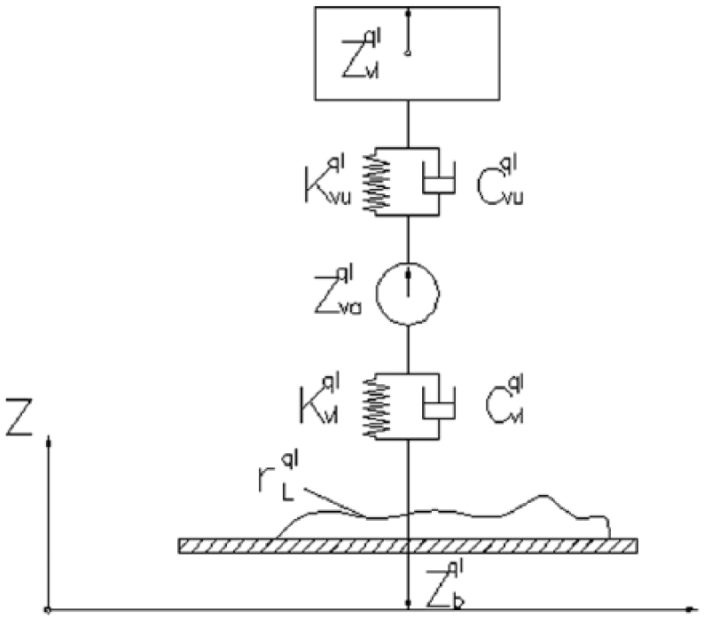
Based on the 3D vehicle model with 12 DOFs developed by Yin et al. (2011), in this study, a new full-scale vehicle model with 18 DOFs was developed which includes a 3D driver seat model and can simulate the longitudinal vibration of the vehicle (Figures 1 and 2). The 18 DOFs include the longitudinal displacements (xt), vertical displacements (zt), lateral displacements (yt), pitching rotations (θt), roll displacements (φt), and yawing angle (φt) of the vehicle body, and the longitudinal displacement
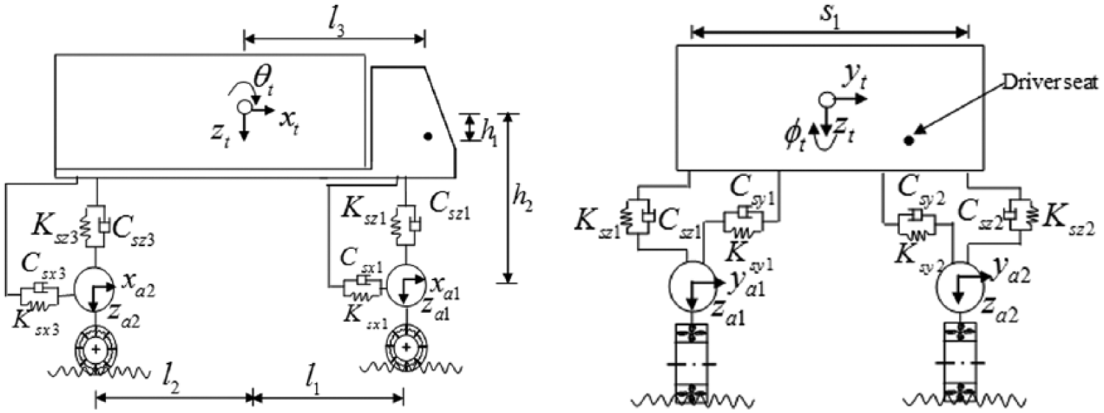
A new full-scale vehicle model.
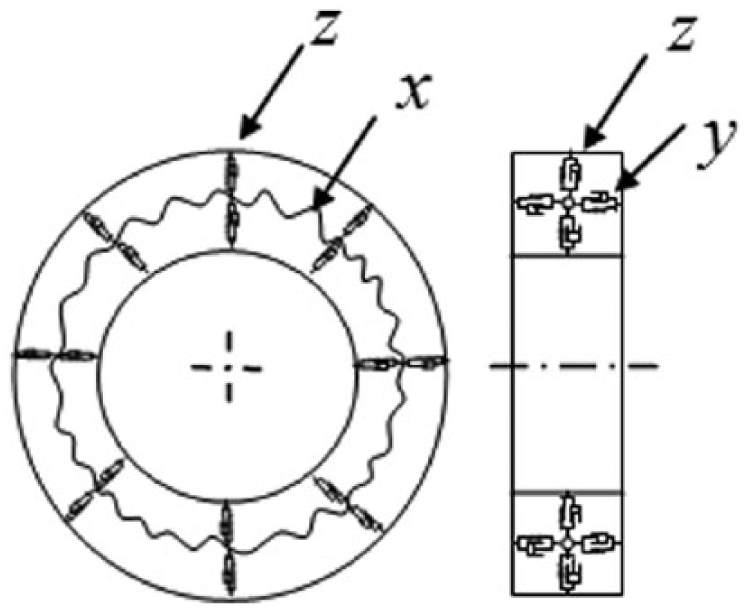
Schematic diagram of the tire model: longitudinal springs (x), lateral springs (y), and radial springs (z).
To simulate the interaction between the vehicle wheel and road surface, the wheel was modeled as a 3D elementary spring as shown in Figure 3, and the mass of the wheel was included in the mass of the axle.
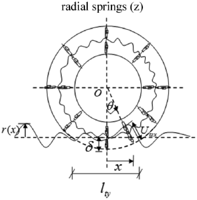
Schematic diagram of wheel deformation.
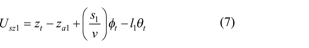
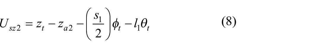
The displacement in the radial direction of the wheel spring (see Figure 3) at the contact position x can be expressed as
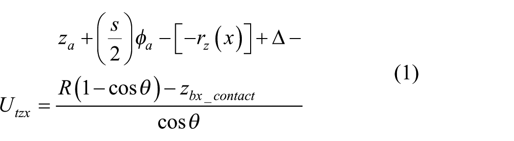
where Utzx is the radial deformation of the wheel at the position x; s is the distance between the right and left wheels; and


where Ftz is the elastic force due to the vertical deformation of the wheel, Fdtz is the damping force due to the vertical deformation of the wheel, ktz is the spring stiffness of the wheel in the radial direction, and ctz is the damping coefficient of the wheel in the radial direction.
The interaction vertical force Fv−b acting on the wheel can be obtained as

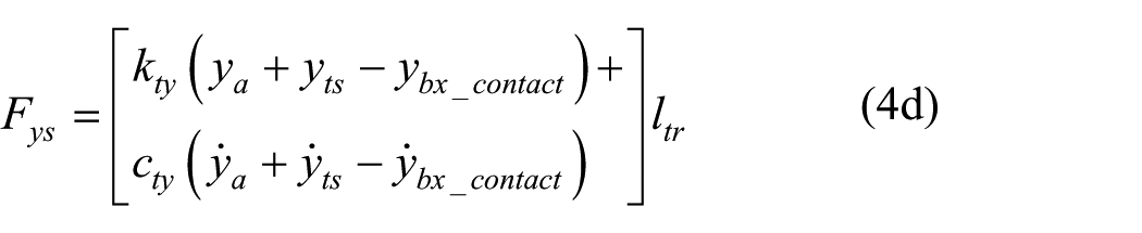
According to Gim and Nikravesh (1990), the lateral force of a pneumatic tire–road surface interaction can be considered as a resultant force composed of three components, that is, Fys, Fyα, and Fyγ due to the tire running with an “S” shape, slip angle α, and camber angle γ, respectively. The lateral force can be obtained as (see more description and definition in Gim and Nikravesh (1990))

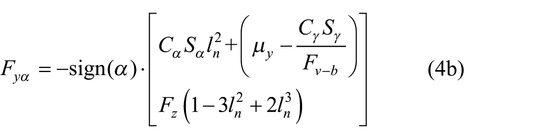

where Cα is the cornering stiffness, Sα is the absolute value of the lateral slip ratio Ssy, ln is a non-dimensional contact patch length and is defined as
The problem of simulating the tire running with an “S” shape is very complex. In this study, to simplify the model, the “S” shape was assumed as a “Sine” shape with a random amplitude and random phase angle, similar to the assumptions made in Fujii et al. (1975). As a result,

where As is a random amplitude, ls is the wavelength, and φs is the initial phase angle. Based on the study of Fujii et al. (1975), As can be assumed to follow a symmetrical distribution from 2.5 to 5 mm, ls can be obtained from a symmetrical distribution from 6.65 to 10 m, and φs can also be assumed to follow a symmetrical distribution from 0 to 2π.
The longitudinal force of a pneumatic tire–road surface interaction can be considered as a resultant force due to the longitudinal deformation and longitudinal friction of the tire. The longitudinal force can be obtained as

where CS is the longitudinal stiffness, Sn is the absolute value of the longitudinal slip ratio Ssx, ln is the non-dimensional contact patch length, µx is the tire–road surface friction coefficient in the longitudinal (x) direction, and Fz is the tire vertical force acting on the road surface and is equal to “−Fv − b.”
The vertical displacements of the suspension springs can be written as
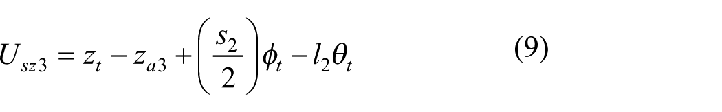

where l1 is the distance between the front and the center of the vehicle, l2 is the distance between the rear axle and the center of the vehicle, and s1 and s2 are the distance between the right and left axles, respectively.
The vertical elastic and damping forces of the suspension can be written as


where Kszi and Cszi are the suspension spring stiffness and damping of the ith axle, respectively.
The lateral and longitudinal displacements of the suspension springs can be written as

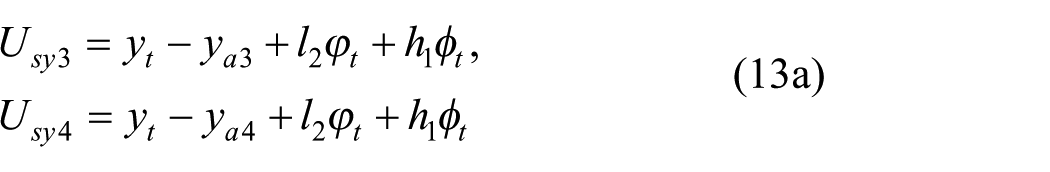

where h1 is the vertical distance of the vehicle center to the driver seat.
The lateral and longitudinal elastic and damping forces of the suspension can be written as


The equations of motion of the full-scale vehicle can be obtained from the Lagrangian formulation and can be written as
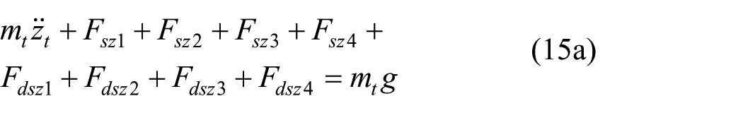
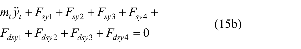

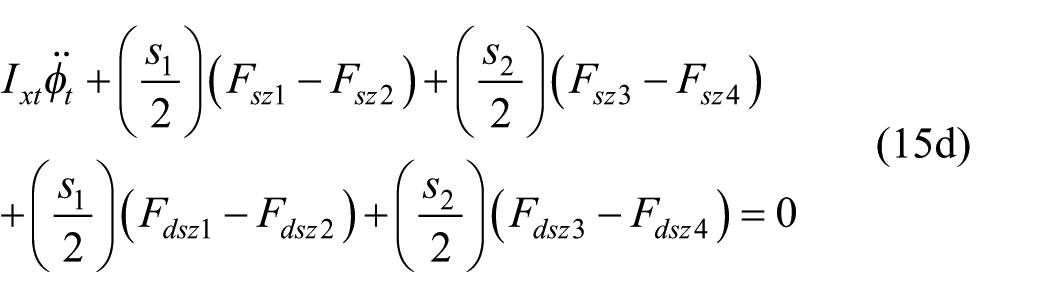
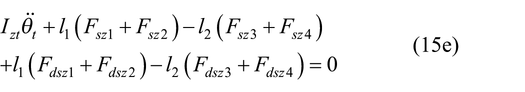
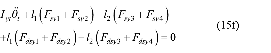


where mt and mai represent the masses of the vehicle body and the ith axle, respectively.
Equations (15a)–(15i) can be rewritten in a matrix form as
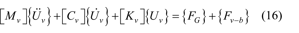
where [Mv], [Cv], and [Kv] are the mass, damping, and stiffness matrices of the vehicle, respectively; {Uv} is the displacement vector of the vehicle; {FG} is the gravity force vector of the vehicle; and {Fv−b} is the vector of the wheel–road contact forces acting on the vehicle.
Equations of motion of bridge model
The equation of motion of a bridge can be written as

where
Assembling the vehicle–bridge coupled system
Using the displacement relationship and the interaction force relationship at the contact patches, the vehicle–bridge coupled system can be established by combining the equations of motion of both the bridge and vehicles (Yin et al., 2011), as shown below
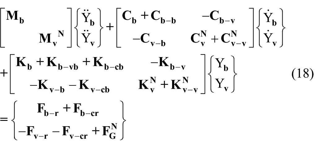
where
EDWL approach
As mentioned by Chen and Cai (2007), the vehicle–bridge coupled equation (18) can consider a number of vehicles of various types at any location on the bridge. When the real traffic flow is simulated, the parameters of each vehicle will be integrated into equation (18) for a “fully coupled” traffic-bridge dynamic interaction analysis. In order to improve the computational efficiency of the analysis, the EDWL approach proposed by Chen and Cai (2007) was adopted in this study. Using this method, the impact of the vehicles, which were previously modeled as mass–spring–damper systems, was replaced with individual time-variant equivalent dynamic moving forces. In this way, solving the “fully coupled” traffic-bridge coupling equations was not required. As a result, the “fully coupled” traffic-bridge model as shown in equation (18) can be simplified as did by Chen and Cai (2007)

where {F} wheel Eq is the collective EDWL of all the vehicles moving on the bridge at a point of time, Csb and Ksb represent the damping and stiffness matrices of the bridge considering the elastic damping and stiffness components, respectively. Essentially, the EDWL approach is to superimpose all the individual equivalent time-variant moving forces of vehicles acting on the bridge at any time to estimate the joint dynamic impacts on the bridge induced by the traffic flow. The individual equivalent force for each moving vehicle is obtained through fully coupled bridge/vehicle analysis in the time domain. The CA traffic model introduced in the previous section provides the detailed speed and location information of each individual vehicle of the random traffic flow on the bridge. Detailed information about the interaction model using EDWL can be found in Chen and Cai (2007).
Traffic flow simulation results by considering the influence of the next-nearest neighbor vehicle
The simulation of CA traffic model can capture the basic features of probabilistic traffic flows by adopting the realistic traffic rules such as car-following and lane-changing, as well as the actual speed limits. One of the most important CA models is the Nagel–Schreckenberg (NaSch) model proposed by Nagel and Schreckenberg (1992) in 1992. Although the NaSch model is simple, it can describe some traffic phenomena in reality, such as phase transition. In recent years, the CA-based traffic flow simulation model was introduced to study the vibration of bridge under the traffic flow and satisfactory accuracy was achieved (Chen and Wu, 2010). However, all previous CA models did not take into account the influence of the next-nearest neighbor vehicle, which cannot be ignored because of its influence on the real traffic (Kong et al., 2006). In this article, an improved CA model that can consider the influence of the next-nearest neighbor vehicle, which was proposed in Kong et al. (2006), was used to simulate the traffic flow.
In the car-following model, most researchers consider the influence of the vehicle ahead using the following equation (Kong et al., 2006)

where T is a response time lag, λ is the sensitivity coefficient,

where T1 is a response time lag of the nearest neighbor vehicle ahead, T2 is a response time lag of the next-nearest neighbor vehicle ahead, and λ1 and λ2 are the sensitivity coefficients corresponding to T1 and T2, respectively, and both of them are confined from 0 to 1 and λ1 > λ2. Using equation (21), the rules for the acceleration/deceleration can be changed in the NaSch model.
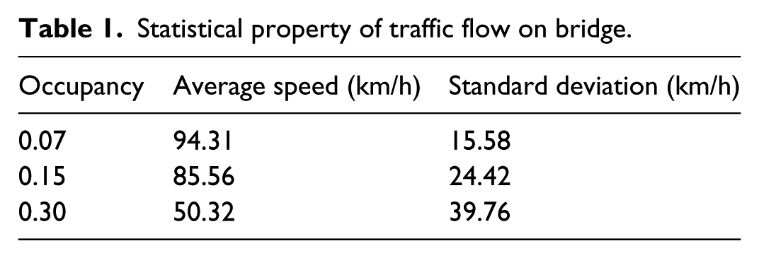
Based on equation (21), the two-lane CA model considering the influence of next-nearest neighbor vehicle was established for the tested highway bridge. As mentioned in the study by Chen and Cai (2007), in order to develop the EDWL database, all the vehicles were classified into three types: (1) v1-heavy multi-axle trucks, (2) v2-light trucks and buses, and (3) v3-sedan cars. In this study, to simplify the vehicular model, only heavy trucks were modeled with 3D vehicle models, while light trucks and sedan cars were modeled with the quarter vehicle models to save computational efforts. A similar bridge was selected as the prototype bridge used in the previous study by Chen and Cai (2007). The approaching roadway at each end of the bridge is assumed to be 1005 m, the speed limit of the highway system can be assumed as 135 km/h, which is converted to the maximum velocity of vehicles in CA model as 5 cell/s. The sensitivity coefficients of the nearest neighbor and next-nearest neighbor vehicle are λ1 = 0.2 and λ2 = 0.05, respectively (Kong et al., 2006). The traffic flow simulation results with the CA model usually become stable after a continuous simulation with a period that equals to 10 times the cell numbers of the traffic simulating system (Chen and Cai, 2007; Nagel and Schreckenberg, 1992). For the purpose of comparison, two different vehicle occupancy coefficients ρ are considered (Chen and Wu, 2011): median traffic (ρ = 0.15) and busy traffic flow (ρ = 0.3). It can be found from Figure 4 that the x-axis and y-axis represent the coordinates in the spatial and time domains, respectively, with each dot on the figures representing a vehicle; with the increase in the traffic occupancy, local congestions may be resulted at some locations as indicated by black belts in Figure 4. It is easily found from Table 1 that the mean speed of the traffic flow decreases while the standard deviation of the vehicle speeds increases with the increase in the vehicle occupancy.
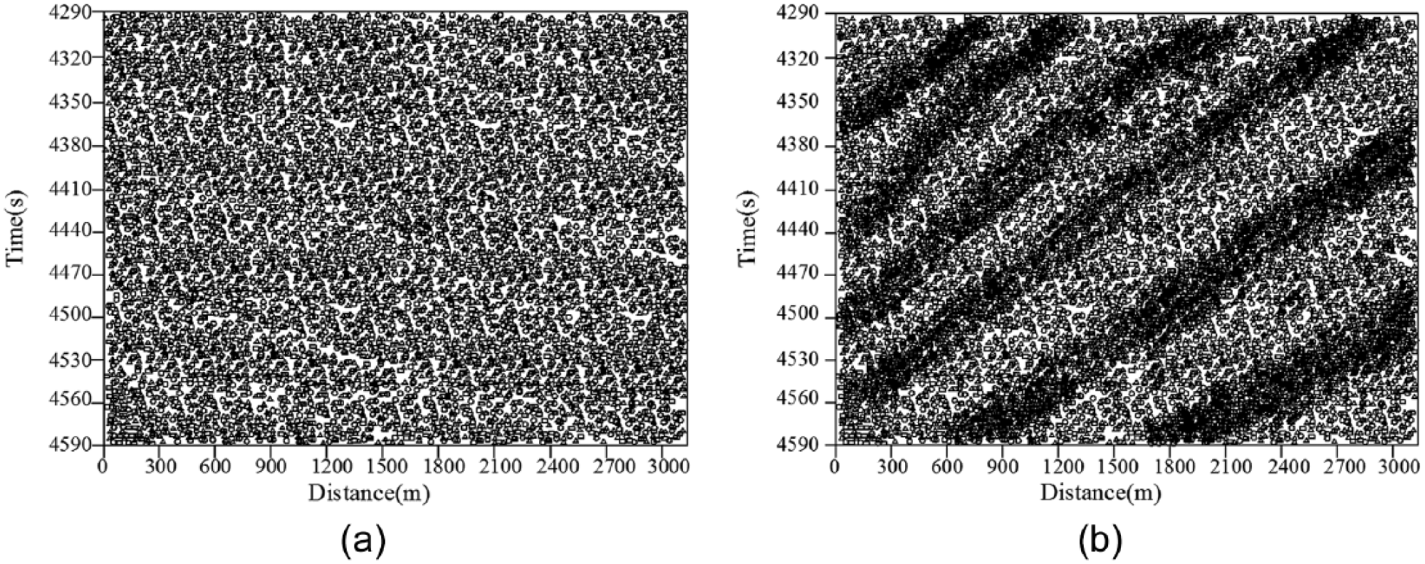
Traffic simulation with different vehicle occupancies: (a) median traffic flow and (b) busy traffic flow.
Statistical property of traffic flow on bridge.
Modeling of progressive deterioration for road surface
The road surface condition is an important factor that affects the dynamic responses of both the bridge and vehicles. The road surface profile is usually assumed to be a zero-mean stationary Gaussian random process and can be generated through an inverse Fourier transformation based on a power spectral density (PSD) function (Yin et al., 2011) as

where

where n is the spatial frequency (cycle/m), n0 is the discontinuity frequency of 1/2π (cycle/m), ϕ(n0) is the roughness coefficient (m3/cycle) whose value is chosen depending on the road condition, and n1 and n2 are the lower and upper cut-off frequencies, respectively. The International Organization for Standardization (ISO) (1995) has proposed a road roughness classification index from A (very good) to E (very poor) according to different values of ϕ(n0).
In order to consider the deterioration of road surface damages due to external loads or environmental attack/corrosion, a progressive deterioration model for the road roughness is necessary. To conduct the fatigue reliability assessment for existing bridges considering road surface conditions, a progressive deterioration model of road roughness changing with time was proposed by Zhang and Cai (2012), which was used in this study as shown below

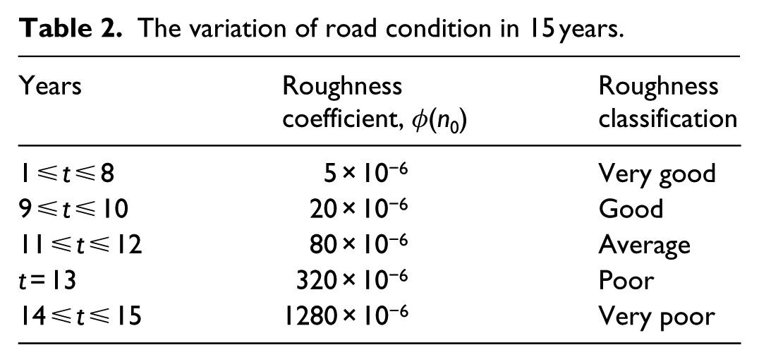
where IRI0 is the initial roughness value upon completing the construction and before opening to traffic; t is the time in years; η is an environmental coefficient that varies from 0.01 to 0.7 depending on dry or wet, freezing or nonfreezing conditions; SNC is a parameter calculated from the data on the strength and thickness of each layer in the pavement; and (CESAL) t is the estimated number of trucks in terms of an equivalent AASHTO single axle load of 80 kN (18 kip) at time t in millions and can change with the traffic increase rate α. Using equation (24), the calculated results of the roughness coefficients and their corresponding classifications are summarized in Table 2. The samples of road roughness profiles can be obtained using equation (22) and are shown in Figure 5. The road condition was classified as very good in the first 8 years, good in the 9th and 10th years, average in the 11th and 12th years, poor in the 13th year, and very poor in the 14th and 15th years.
The variation of road condition in 15 years.

Road roughness profile samples: (a) road roughness profile in the first 8 years, (b) road roughness profile in 11th and 12th years, and (c) road roughness profile in the 13th year.
Field test studies and numerical studies
Description of an existing bridge
A five-span reinforced concrete continuous bridge constructed in 1980 was investigated in this study. It is located in the Changde County, Hunan Province, China. The bridge has a total length of 350 m and a bridge width of 10 m, and a span configuration of 55 + 70 + 90 + 80 + 55 m. The bridge was designed to carry the load of vehicle–20 in the CHBDC. Large deflection and lots of cracks were observed during an inspection of the bridge conducted in 2001, indicating that this bridge had been deteriorated severely after a long service time in harsh conditions. The bridge was then repaired in 2001. After another 10 years of service, static and dynamic tests were conducted again to evaluate the bridge safety in June 2011 (Figure 6).
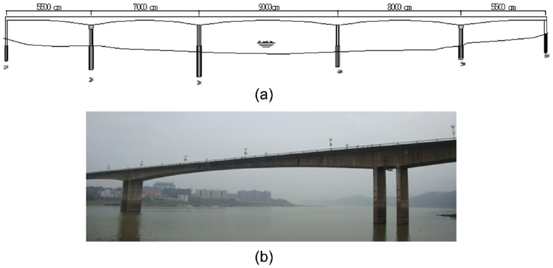
The tested bridge: (a) configuration of the bridge and (b) longest span of tested bridge.
Road surface condition
The road surface condition is an important factor that affects the dynamic responses of both the bridge and vehicles (Yin et al., 2011; Yu and Chan, 2007). In order to examine the effect of road roughness on the accuracy of the present method, the road roughness of the bridge was measured using a similar method as those used in references (ISO, 1995; Yin et al., 2011). Figure 7 shows two pictures of the road surface condition of the bridge taken in 2001 and 2011, respectively, while Figure 8 shows the measured road roughness profiles. From Figures 7 and 8, it can be seen that the road surface on the bridge experienced serious deteriorations during a period of 10 years, and the corresponding road roughness classification changed from very good in 2001 to poor in 2011.
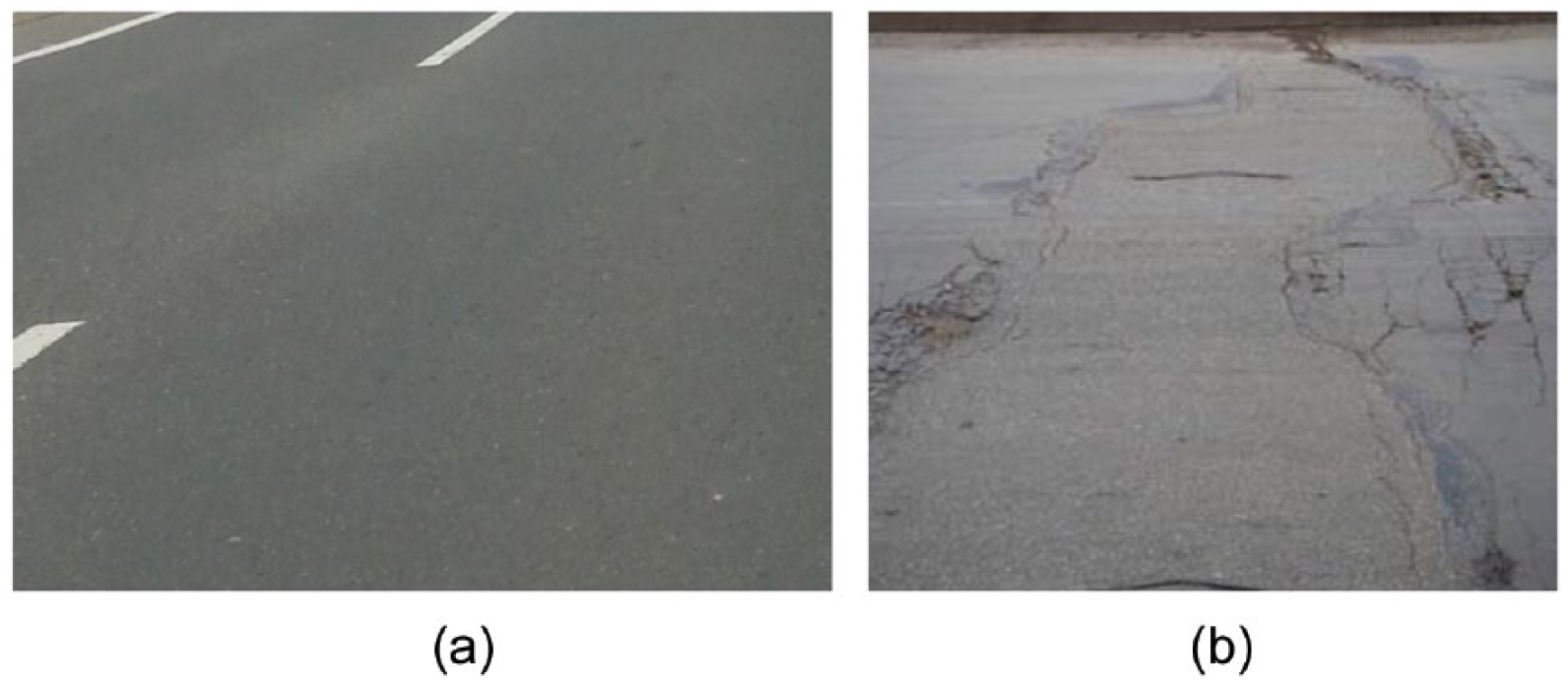
Road surface of the bridge deck: (a) the road surface in 2001 And (b) the road surface in 2011.
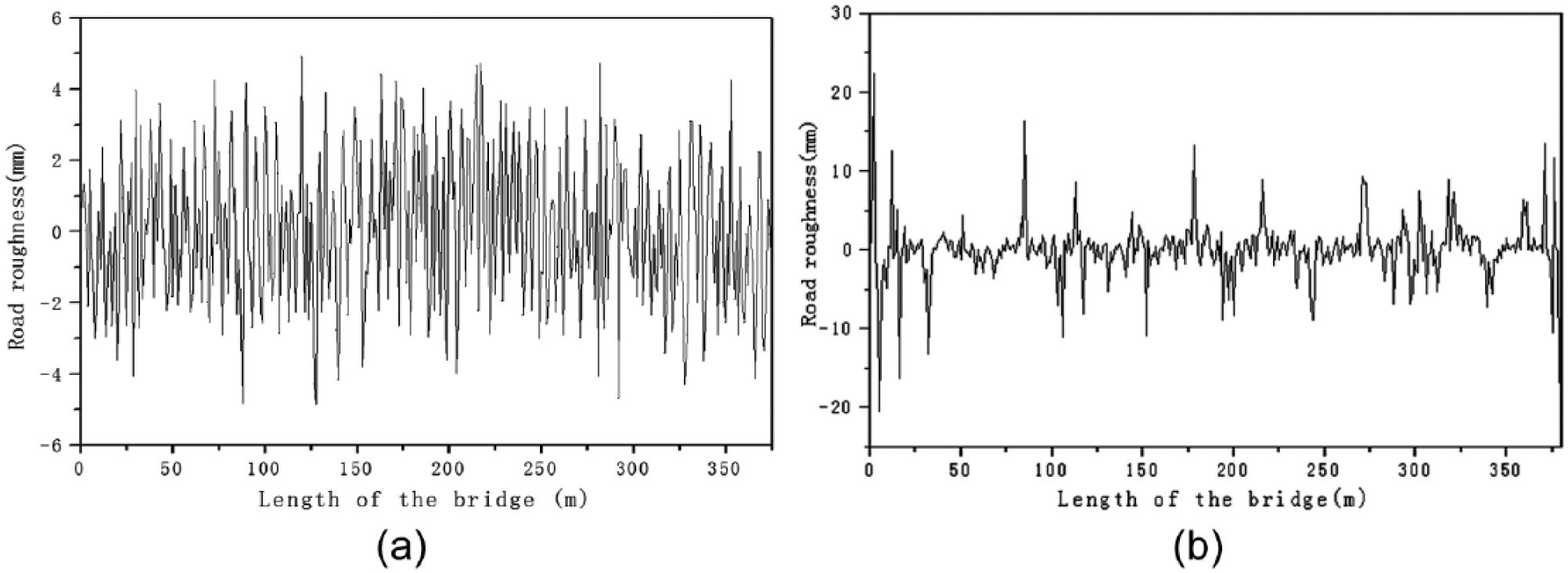
Road roughness of the tested bridge: (a) the measured road roughness profile in 2001 and (b) the measured road roughness profile in 2011.
Bridge model updating
Based on the configuration of the bridge, a finite element (FE) model was created for this bridge, as shown in Figure 9. Before being used in the numerical simulation, the FE bridge model was updated based on the results of a modal test performed using the ambient vibration method. The details of the experiment setup and model updating can be seen in Yin et al. (2011).
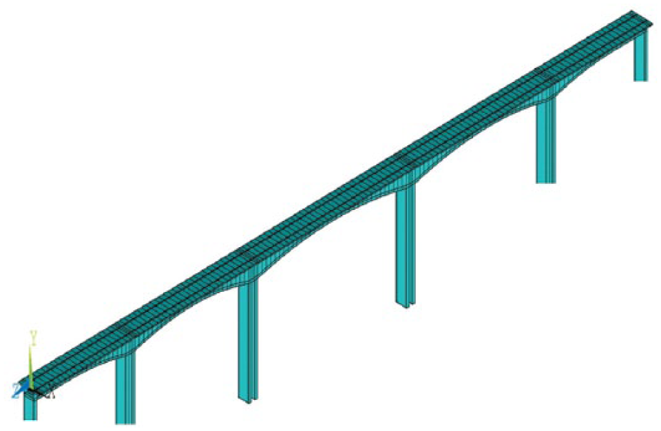
The finite element model of the tested bridge.
The parameters of traffic vehicles
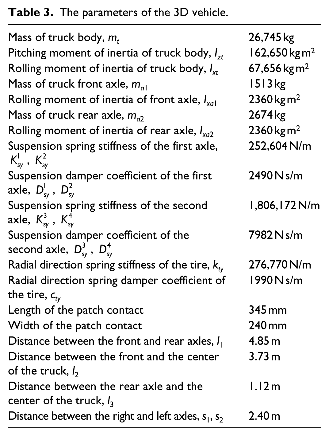
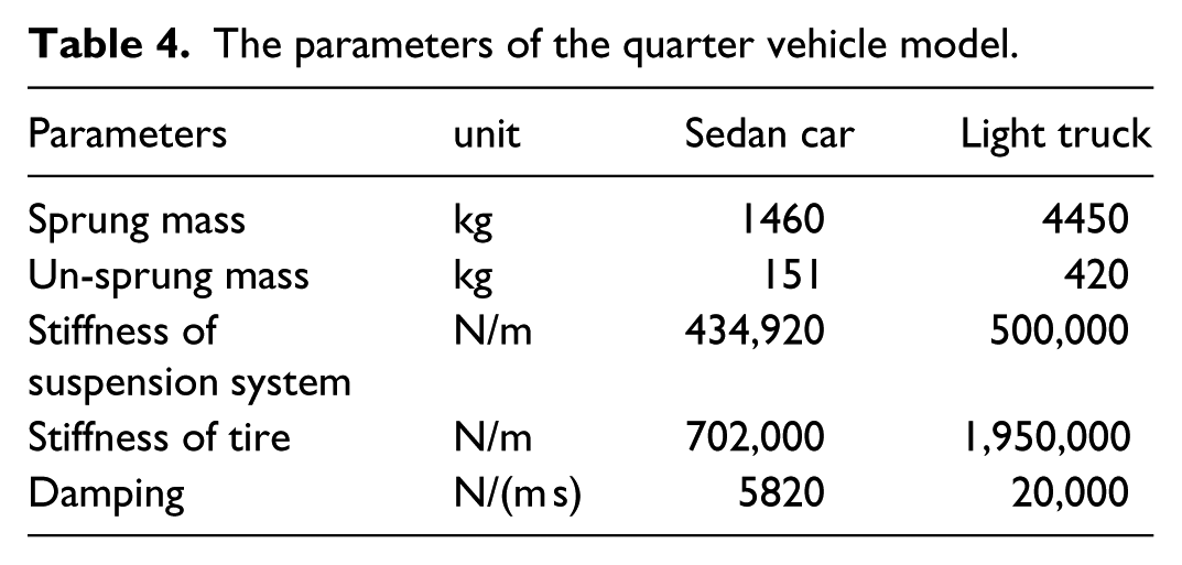
As mentioned in Chen and Cai (2007), in order to develop the EDWL database, all the vehicles are classified into three types: (1) v1-heavy multi-axle trucks, (2) v2-light trucks and buses, and (3) v3-sedan cars, and the percentage of three types of vehicles v1, v2, and v3 are equal to 0.2, 0.3, and 0.5, respectively. In this study, to simplify the vehicular model, only heavy trucks are modeled with 3D vehicle models, while light trucks and sedan cars are modeled using quarter vehicle models to save computational efforts. The 3D vehicle model and the quarter vehicle model are shown in Figures 1 and 10, respectively, and the parameters of the vehicle models are summarized in Tables 3 and 4. The mechanical and geometric properties of the test truck can be obtained from Yin et al. (2011) and are listed in Table 3. The parameters of the quarter vehicle model can be obtain from Chen and Cai (2007) and are also shown in Table 4.
The quarter vehicle model used in Chen and Cai (2007).
The parameters of the 3D vehicle.
The parameters of the quarter vehicle model.
The comparison of the bridge responses under three traffic flow occupancies
In this section, three levels of traffic flow occupancies are used to study the bridge responses under the tested road surface roughness shown in Figure 8(a). Three traffic flow occupancies, that is, smooth traffic with ρ = 0.07, median traffic with ρ = 0.15, and busy traffic flow with ρ = 0.3, are usually used in previous studies (e.g. Chen and Wu, 2011). The time histories of the vertical and lateral displacements at the mid-span of bridge are presented in Figure 11 under the three traffic flow occupancies and the same road surface condition shown in Figure 8(a).
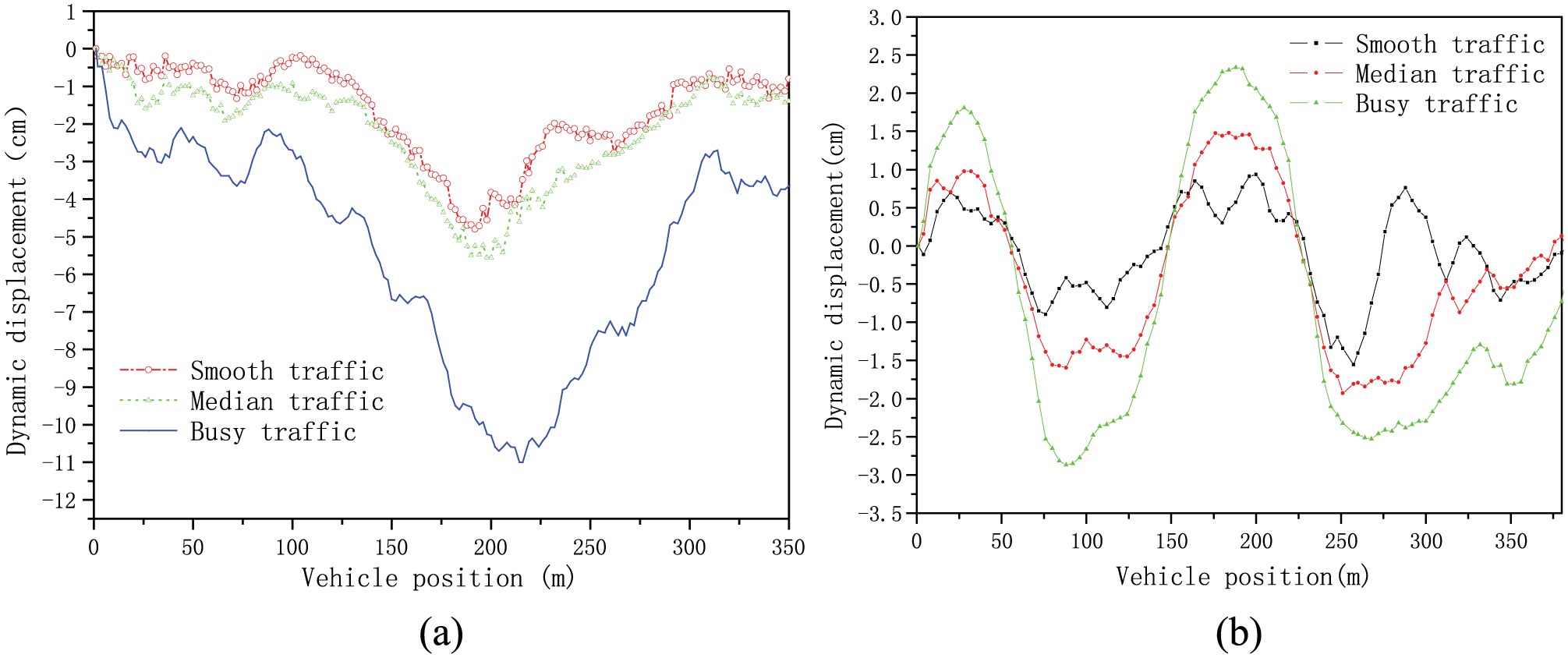
The bridge responses under three levels of traffic flow occupancies: (a) vertical displacements of bridge and (b) lateral displacements of bridge.
It is found that both the vertical and lateral displacements at the mid-span generally increase with the increase in vehicle occupancy; thus, the vehicle occupancy plays a significant role on the bridge displacements. For example, the maximal vertical displacement of bridge increases from 4.86 to 11.06 cm when the vehicle occupancy increases from smooth traffic to busy traffic.
Comparison of bridge responses under different service years
In this section, the effect of service years on the vertical and lateral displacements at the mid-span of bridge is examined. Median traffic flow occupancy, traffic increase rates, and progressive deterioration model of road roughness were used. The results are presented in Figure 12 for three different numbers of years in service.
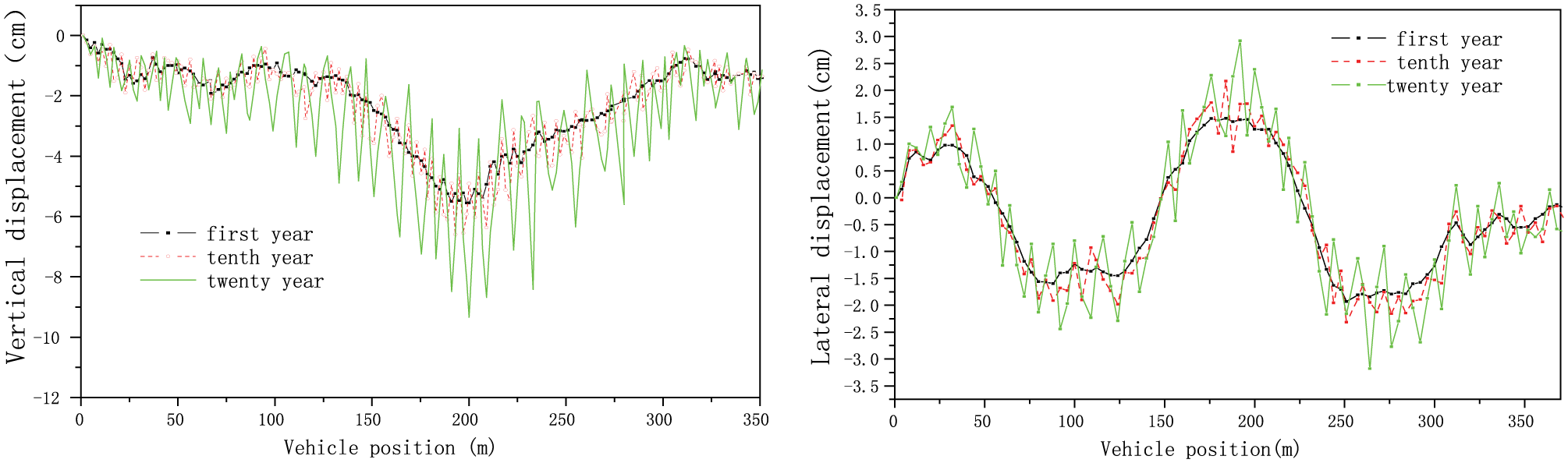
The bridge responses under increasing years (α = 0, median traffic).
It is found that the displacement at the mid-span increases significantly with the increase in service years of the bridge. The maximal vertical displacement of bridge increases from 5.62 cm in the first year to 9.34 cm in the 20th year of service, and the maximal lateral displacement of bridge increases from 1.91 to 3.19 cm for the same period of time.
Comparison of bridge responses under the combined effect of service years and traffic increases
The vertical and lateral displacements at the mid-span of bridge under median traffic flow occupancy and different traffic increase rates (3% and 5%), which obtained from Zhang and Cai (2012), are presented in Figures 13 and 14.
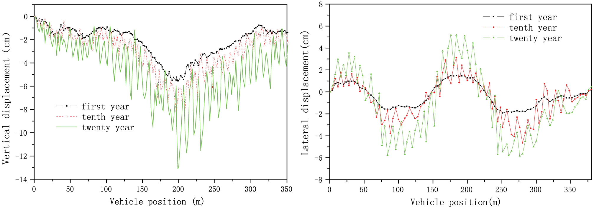
The bridge responses under different years of service (α = 3%, median traffic).
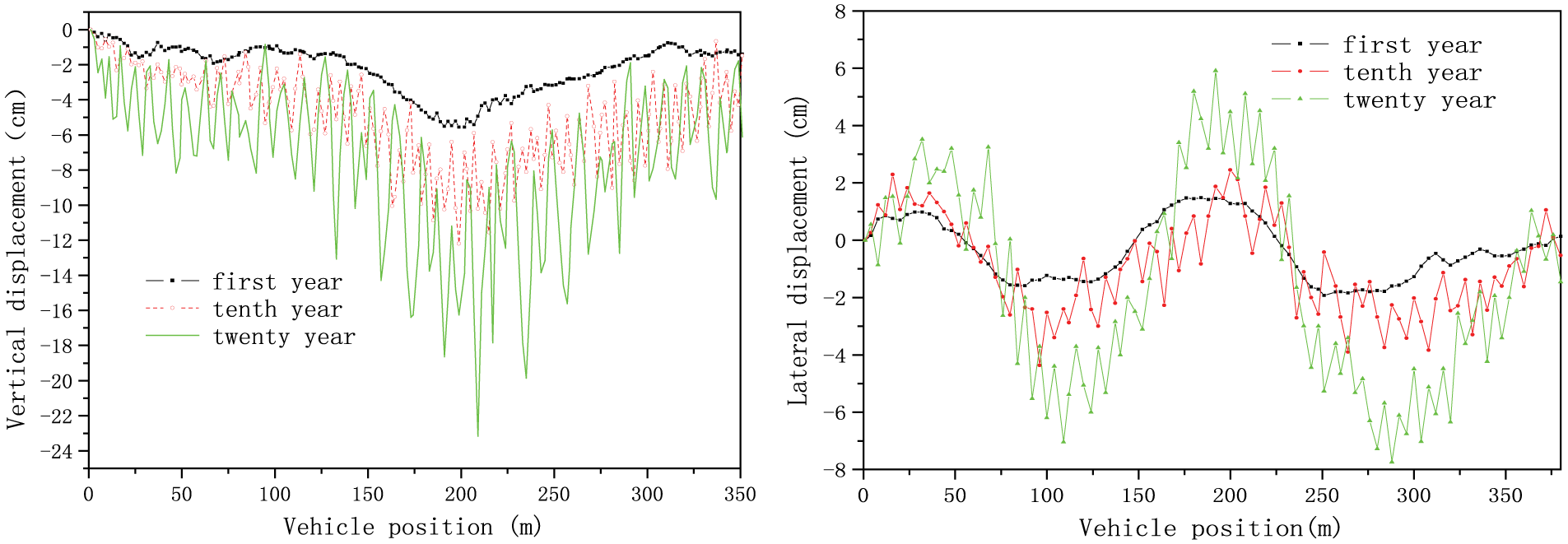
The bridge responses under different years of service (α = 5%, median traffic).
It is found that the displacements at the mid-span increase significantly with the increase in service years. The maximal vertical displacement of the bridge increases from 5.62 cm in the first year to 13.06 cm in the 20th year of service under a traffic increase rate α = 3%. Correspondingly the maximal lateral displacement of the bridge increases from 1.91 to 5.83 cm. Based on the comparing between Figures 13 and 14, it can be observed that the traffic increase rate also affects the responses of the bridge.
Comparison of impact factors under the combined effect of service years and traffic flow occupancies
As mentioned before, the impact factors in the design codes are usually aimed at providing guidelines for designing new bridges. However, for a large majority of old bridges whose road surface conditions have deteriorated due to factors like aging, corrosion, and increased traffic load, caution should be taken when using the code-specified impact factors. Therefore, for safety purposes, more appropriate impact factors should be provided for these old bridges. Deng (2009) proposed a function of impact factor for the old bridges with respect to bridge span length and bridge surface roughness. However, their study was based on simply supported bridge, and more theoretical support was also needed for the proposed impact factor functions. In this study, the impact factor is defined as follows

where Rd(x) and Rs(x) are the maximum dynamic and static responses of the bridge at location x, respectively.
The effect of service years, three levels of traffic flow occupancies, and three traffic increase rates on the impact factors are presented in Figure 15. It is found that the impact factors increase significantly with the increase in service years, For example, with the median traffic, the impact factor increases from 0.00345 in the first year to 0.123 in the 10th year; however, the effects of traffic flow occupancies and three traffic increase rates on the impact factors are not very significant, For example, when the traffic increase rate equals 0, shown Figure 15(d), the effects of the impact factors are not monotonically increased with the increase in traffic flow occupancies.
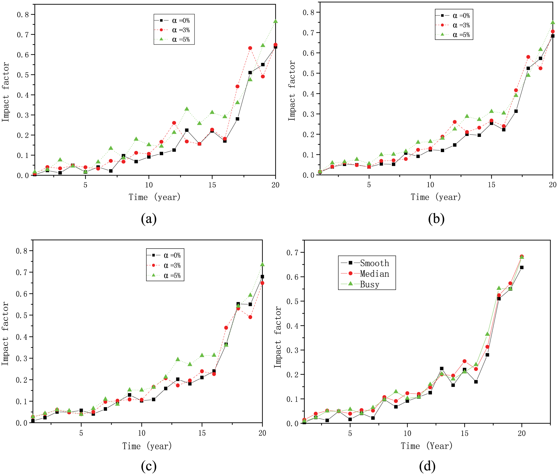
Impact factors under different years of service and traffic flow occupancies: (a) smooth traffic flow with ρ = 0.07, (b) median traffic flow with ρ = 0.15, (c) busy traffic flow with ρ = 0.3, and (d) three traffic flow occupancies α = 0%.
The proposed expression of the impact factor considering the years of service
From the previous sections, it is known that the code-specified impact factors may not be sufficient to reflect the actual dynamic responses for existing bridges, and the dynamic responses of the existing bridges would increase with the increase in years in service. Therefore, for a real bridge structure that has been in service for several years, the actual impact factor may differ from design codes. In this section, based on the current Chinese bridge design codes, impact factors for evaluating the dynamic responses of existing bridges are proposed.
In the CHBDC (2004), the IM is defined as a function of the natural frequency of the bridge as shown below
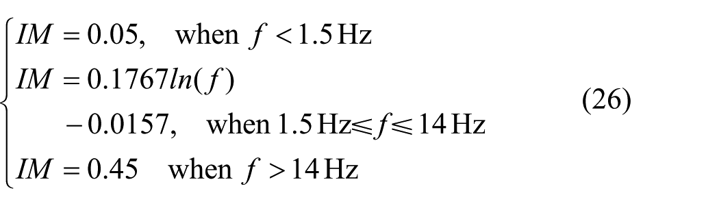
where f is the natural frequency of the bridge.
To reflect the actual impact factor that varies with the number of years in service, a corrected coefficient as a function of time is introduced and can be expressed as

where IM0 is the impact factor defined in the current CHBDC code and IMt is the impact factor calculated from numerical simulation using the present method.
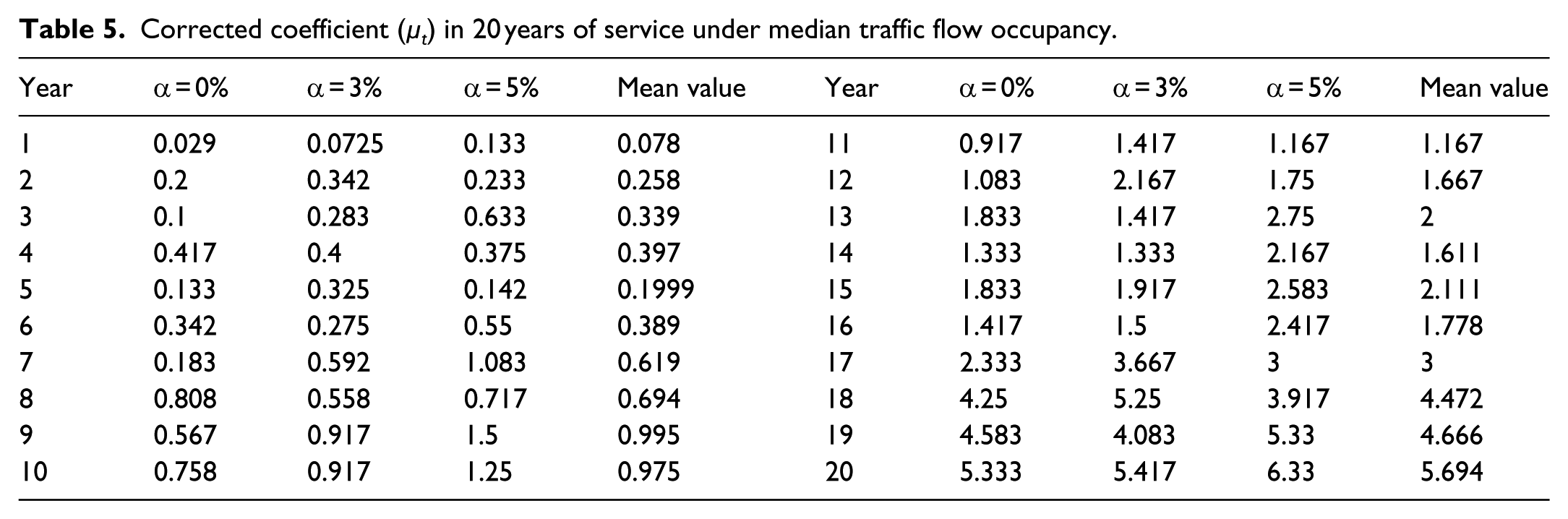
Figure 16 and Table 5 show that the corrected coefficient (µt) increases significantly with the increase in service years, which is similar with the effect of service years on the impact factors. Figure 16(b) shows the comparison of the calculated mean values and the fitted function of the corrected coefficients. To study the effect of service years on the corrected coefficient, a fitted function of service years can be obtained as follows

where t is the service years.
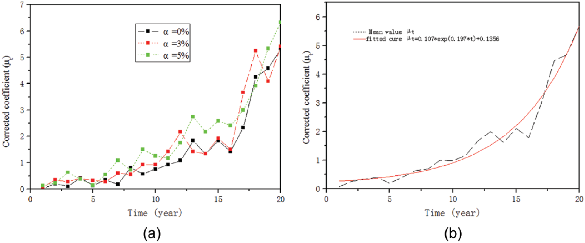
The corrected coefficient (µt) versus the number of years in service: (a) the effect of service years on the corrected coefficient and (b) the comparison of the calculated mean values and the fitted function.
Corrected coefficient (µt) in 20 years of service under median traffic flow occupancy.
Based on the current CHBDC (2004), by introducing the corrected coefficient, new expressions of impact factors are proposed as follows

Impact factors defined in equation (29) can be used for evaluating the dynamic responses of existing bridges. Similar approach may be applied to other bridge design codes.
Conclusion
In this study, a 3D vehicle–bridge coupled model is used to analyze the impact factors of in-service bridges by considering the effect of the stochastic traffic flow and the progressive deterioration for road surface roughness. A 3D vehicle model with 18 DOFs was adopted. An improved CA model considering the influence of the next-nearest neighbor vehicle and a progressive deterioration model for road roughness were introduced. Based on the EDWL approach, the coupled equations of motion of the bridge and traffic flow are established by combining the equations of motion of both the bridge and vehicles using the displacement relationship and interaction force relationship at the patch contact. The numerical simulations show that the proposed method can rationally simulate the impact factor of the bridge under stochastic traffic flows. Expressions of impact factors that can be used to evaluate the dynamic responses in-service bridges are proposed. Based on the results from this study, the following conclusions can be drawn:
An improved and more realistic CA model that considers the influence of the next-nearest neighbor vehicles can be introduced to study the dynamic responses of the bridge.
The vehicle occupancy plays a significant role on the bridge dynamic displacements, and the displacements at the mid-span generally increase with the increase in vehicle occupancies. For example, the maximal vertical displacement of bridge increases from 4.86 to 11.06 cm when the vehicle occupancy increases from the smooth traffic to busy traffic. However, the effects of the impact factors are not monotonically increased with the increase in traffic flow occupancies.
The impact factors increase significantly with the increase in bridge service years due to the deterioration of the road roughness. Under a normal traffic condition, the impact factors can increase from 0.00345 in the first year to 0.123 in the 10th year.
While maintaining the format used for impact factors in the existing Chinese bridge design code, expression of impact factors for in-service bridges was given based on the numerical simulation results. This approach may be applied to other bridge design codes.
Since the road surface condition has proven to have a large influence on the impact factor, regular maintenance of the road surface is a very effective way of reducing vehicle-induced vibration and maintaining the safety of bridges.
Footnotes
Declaration of Conflicting Interests
The author(s) received no financial support for the research, authorship, and/or publication of this article.
Funding
The author(s) disclosed receipt of the following financial support for the research, authorship, and/or publication of this article: This work is supported by the National Basic Research Program of China (973 Program; Project No. 2015CB057702), the Natural Science Foundation China (Project No. 51108045), and Innovation platform of open fund project of Hunan Provincial Education Department of China (Project No. 13k051).