Vibration-based damage identification of an unreinforced masonry house model

Abstract

Non-destructive vibration-based damage identification techniques are especially attractive for assessing damage in structures of high historical and architectural value. So far, most studies have focused on slender structures built using relatively homogeneous materials. In this study, global damage identification methods based on vibration response parameters were applied for identifying damage in an unreinforced masonry full-scale house model (non-homogeneous material and non-slender structure). The house model was dynamically loaded using an eccentric-mass shaker. Structural damage to the walls was initiated by increasing the amplitude of the applied load. At each damage state, a modal test was performed by impacting the walls with a calibrated hammer. Statistically significant variations of modal frequencies and the modal assurance criteria were considered as suitable parameters to identify damage. It was concluded that different sets of modes can be found for different states of damage because of material degradation, change in the support and connectivity conditions, and breaks in the members continuity generated by damage. All these changes are reflected in variations of modal frequencies and modal assurance criteria. It was also established that prior to identifying the damage distribution on the entire building, it was necessary to determine how the modal frequencies were related to each wall.

Keywords

damage identification impact test modal analysis unreinforced masonry

Introduction

Damage has been defined as any change that adversely affects the current or future performance of a system (Farrar and Worden, 2007). Damage is usually related to structural responses that cause material non-linearity. However, the effect of damage is not only observed in post-elastic behaviour of structures, but also the linear response might be perturbed due to degradation of elastic stiffness, loss of mass or changes in the system boundary and connectivity conditions.

A number of non-destructive techniques have been developed in the last three decades to detect damage beyond human naked-eye capacities (e.g. acoustic emissions, ultrasonic emissions or X-ray inspections). Most of these methods focus on assessing the local condition of structural elements, and they require a prior localization of the damage and access to the damaged area. There are other kinds of non-destructive methods that can provide global information about damage in a structure. Global damage identification methods are, in general, based on the observation of changes in the dynamic response of structures, for example, modal frequency, mode shapes, modal curvatures and frequency response functions (Ren and De Roeck, 2002). Assuming that ambient conditions do not significantly affect the system properties, changes in the dynamic response can be interpreted as a symptom of structural damage. The main hypothesis of global damage identification is that variations observed in the elastic response of a system (modal properties) are sufficient evidence to diagnose damage. Therefore, it is not necessary to force the structure into the non-linear range to verify damage.

The non-destructive nature of global damage identification techniques makes them especially attractive for identifying damage in structures of high historical and/or architectural value (Beyen, 2008; Durukal et al., 2003; Gentile and Saisi, 2007; Ramos et al., 2010b). These techniques do not require direct access to the damaged zone, and thus they are particularly convenient from an economic and practical perspective, because damage can be early detected and ‘pre-localized’. The information obtained by applying global damage identification techniques can then be used to decide whether a more detailed local analysis is necessary. However, most damage identification studies have focused on structures built using relatively homogeneous materials (e.g. steel and concrete). Only few studies have taken on the challenge of investigating damage in structures made of composite materials such as masonry (an assembly of bricks and mortar), with even fewer studies considering damage of heritage buildings. Most of this studies use frequency and mode shape parameters to identify damage in slender structures, such as tower and arches (Gentile and Saisi, 2007; Osmancikli et al., 2012; Ramos et al., 2010a), and those studies devoted to non-slender elements employed damage indicators based only on modal frequencies (Beyen, 2008; Ceroni et al., 2014; Durukal et al., 2003; Ramos et al., 2010b).

In our study, global damage identification methods based on vibration response parameters (modal frequencies and mode shapes) were applied for detecting and roughly determining the spatial distribution of damage in an unreinforced masonry (URM) full-scale house model (non-slender structure). The house model was dynamically loaded using an eccentric-mass shaker placed on the roof diaphragm. Structural damage to the walls was initiated by increasing the amplitude of the load applied by the shaker. At different stages of damage, modal tests were performed by impacting the house using a calibrated hammer. The dynamic properties of the structure for the different damage states were extracted from the recorded accelerations. As the impact pulse (input signal) was not recorded, an output-only damage identification technique was employed: Stochastic Subspace Identification (SSI). Two simple vibration-based damage indicators (modal frequency variations and modal assurance criteria (MAC)) were considered and applied to the results obtained from modal tests conducted on the URM house model. These indicators have been previously demonstrated to be effective in identifying damage in simple URM structural elements, such as cantilever wall panels subjected to well-controlled damage conditions (diagonal cut) (Oyarzo-Vera and Chouw, 2013).

Experimental setup

Physical model

An unreinforced clay brick masonry house model was constructed by an independent mason with deliberately minimal intervention by the analyst, with the aim of best replicating the typical construction practice used in New Zealand for the construction of historical URM buildings (Russell and Ingham, 2010). The specimen was built using recycled clay bricks (standard dimensions 230 mm × 110 mm × 75 mm) obtained from demolition sites of old masonry buildings in Auckland, New Zealand. The mortar used to assemble the walls was lime based and had a cement:lime:sand ratio equal to 1:2:9. Although the weak mortar employed in this experiment is currently not recommended for bearing walls (ASTM C270, 2008), it is still common in typical early 20th century heritage constructions in New Zealand (Lumantarna et al., 2014). The use of this mortar mix has been shown to be appropriate for replicating the in situ characteristics of historic unreinforced clay brick masonry buildings in New Zealand (Dizhur and Ingham, 2013). Hence, it is interesting to analyse the performance of this structural form when subjected to dynamic loadings, particularly when considering the devastating effects of the 2010/2011 Canterbury earthquake sequence in New Zealand (Moon et al., 2014). The masonry compressive strength and Young’s modulus were determined by standardized three-brick prism compressive tests (ASTM C1314, 2010) and were 3.9 MPa and 0.71 GPa, respectively.

The house dimensions were 4 m × 4 m in plan. The north, east and west walls had a height of 2.2 m and a thickness of 230 mm (two leaves of bricks), whereas the south wall had a height of 1.9 m and was 110-mm thick (one leaf of bricks). The bricks followed a common bond pattern (header course at every fourth course). The east and west walls had one opening for windows and the north wall had two openings for a window and a door. There were no openings in the south wall.

A timber floor diaphragm that consisted of six equally spaced joists (45 mm × 140 mm) supported by the interior leaf of the east and west walls was located at a height of 1.60 m. These joists were connected by four equally spaced lines of blocking (45 mm × 140 mm). The diaphragm flooring was constructed over the joists using timber boards (32 mm × 140 mm) covered by 12 mm plywood sheets simulating a retrofit solution typically applied to floor diaphragms in New Zealand (Wilson et al., 2013). The general dimensions of the walls and the diaphragm layout are shown in Figure 1.

Figure 1.

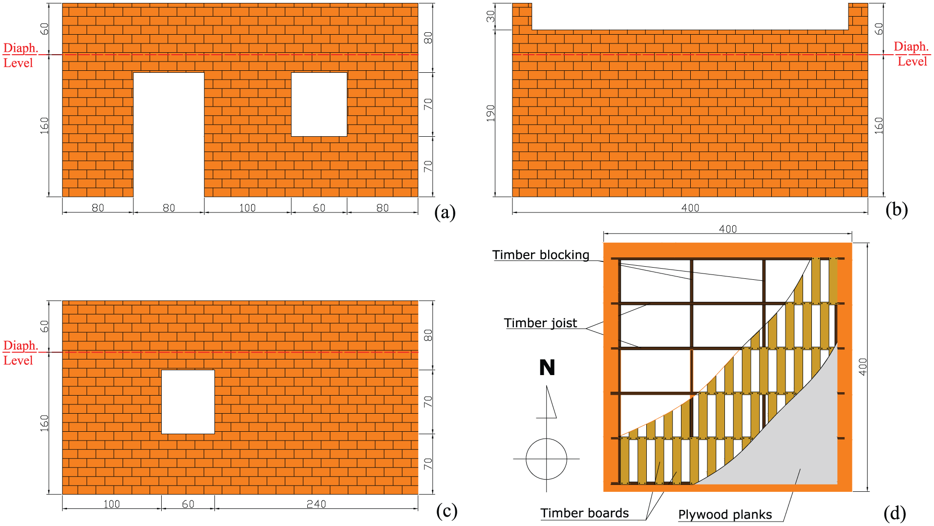
URM house wall dimensions: (a) north wall, (b) south wall, (c) east and west walls and (d) diaphragm layout (all dimensions are in cm).

Dynamic excitation inducing damage

An eccentric-mass shaker (ANCO MK-140-10-50) attached to the roof diaphragm was used to generate an excitation strong enough to create damage on the structure (Figure 2). The purpose of using a shaker to damage the house model was to produce a random, but controlled, deterioration of the walls.

Figure 2.

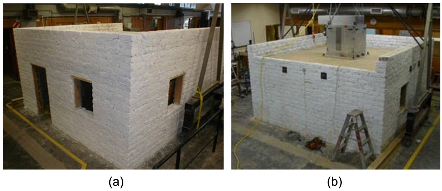
(a) North-west view of URM house model and (b) south-east view of the house model with the eccentric-mass shaker attached to the roof.

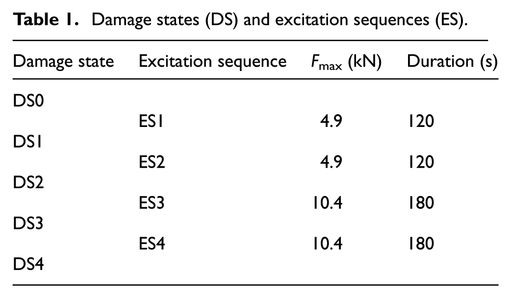
Four horizontal harmonic excitation sequences (ES1–ES4) were applied by the shakers in the north–south direction. Within each excitation sequence, the magnitude of the excitation was gradually increased up to a maximum load (F_max) in a certain time span (duration), as given in Table 1. It is important to note that the setup employed in this experiment was not comparable to a seismic test because the shaker applied the excitation directly to the specimen’s roof instead of activating inertia forces distributed on the walls by applying ground motions. A shake table test would be a more suitable alternative to adequately replicate earthquake conditions. However, it was not the intention of this test to replicate earthquake excitations, but instead to generate controlled random damage that could then be detected by the damage identification procedures under investigation. It is important to remark that shaker’s excitations were not used to perform modal testing and they were applied only to generate damage.

Table 1.

Damage states (DS) and excitation sequences (ES).

Damage state	Excitation sequence	F_max (kN)	Duration (s)
DS0
	ES1	4.9	120
DS1
	ES2	4.9	120
DS2
	ES3	10.4	180
DS3
	ES4	10.4	180
DS4

Modal test and system identification

Although the in-plane shear capacity of walls contributes more significantly to the global strength of a building, walls are more easily excitable in the out-of-plane direction. In addition, it must be noted that damage usually affects more significantly the out-of-plane response of URM walls and, eventually, an out-of-plane failure could be observed prior to an in-plane failure. Hence, it was decided to record only the out-of-plane wall response when performing modal tests in this study.

Modal tests were conducted before loading the structure (DS0) and after each excitation sequence to determine the dynamic properties of the structure (modal frequencies and mode shapes) at different states of damage (DS1–DS4). The modal tests consisted of exciting the structure by impacts with a calibrated hammer (Dytran 5803A) and recording the vibration response using accelerometers (Crossbow CXL02LF1Z and CXL10HF1Z). A total of six hits per wall was applied, two at each of the locations (H1, H2 and H3) as indicated in Figure 3. The structural response was recorded for 30 s at a sampling frequency of 500 Hz in the direction normal to the wall face over a grid of 20 measure points per wall, as also displayed in Figure 3. Although the walls were later analysed independently, reference accelerometers were permanently placed at grid points N8, S8, W8 and E8 to facilitate the comparison between tests and for superposing the results of every instrumental setup. The excitation signal was recorded, but it was not considered for system identification. Nevertheless, it was verified that excitation signal presents a relatively constant power spectral density in the range of frequency to be identified (Figure 4).

Figure 3.

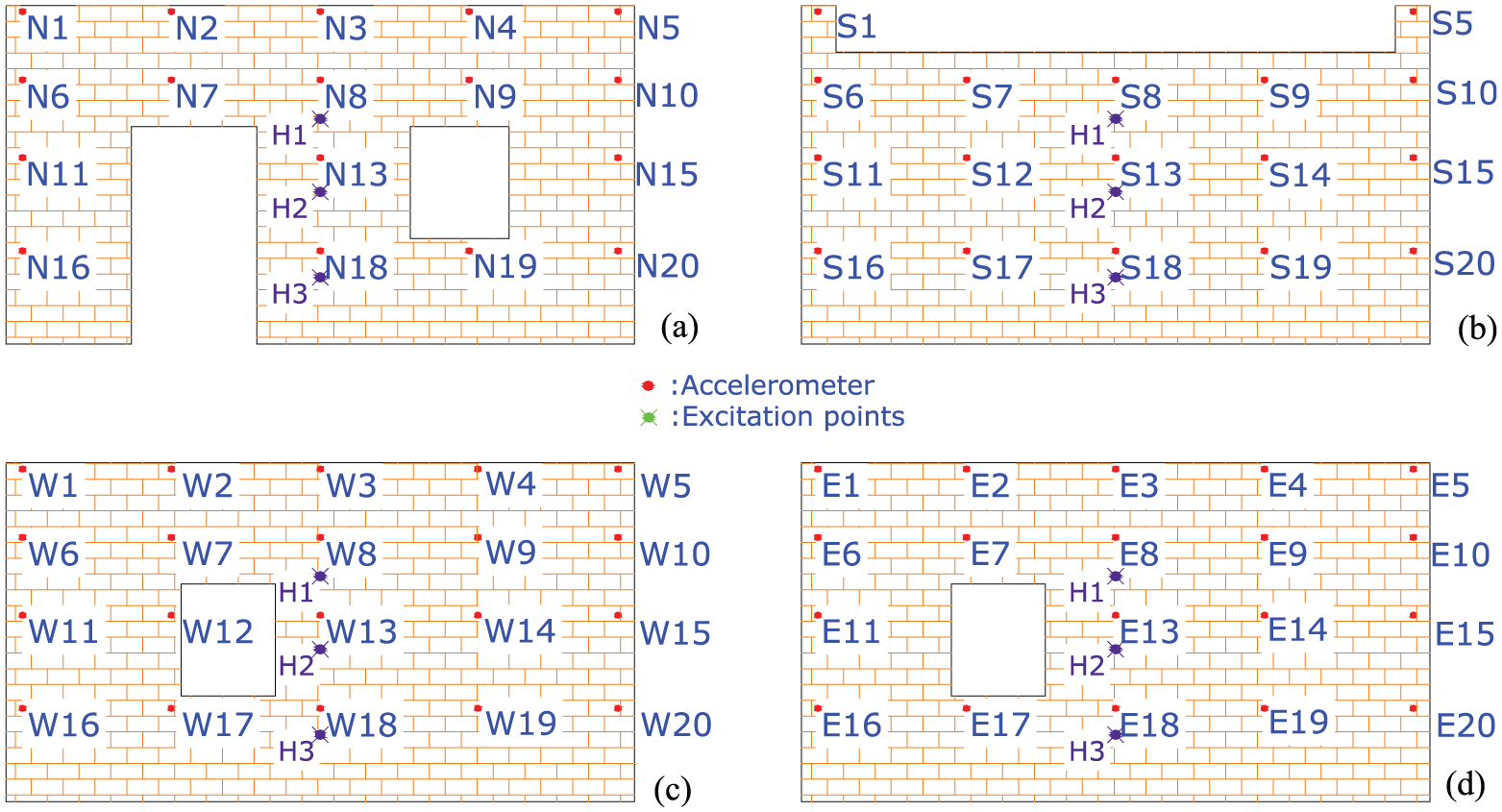
Measurement grid and excitation points: (a) north wall, (b) south wall, (c) west wall and (d) east wall.

Figure 4.

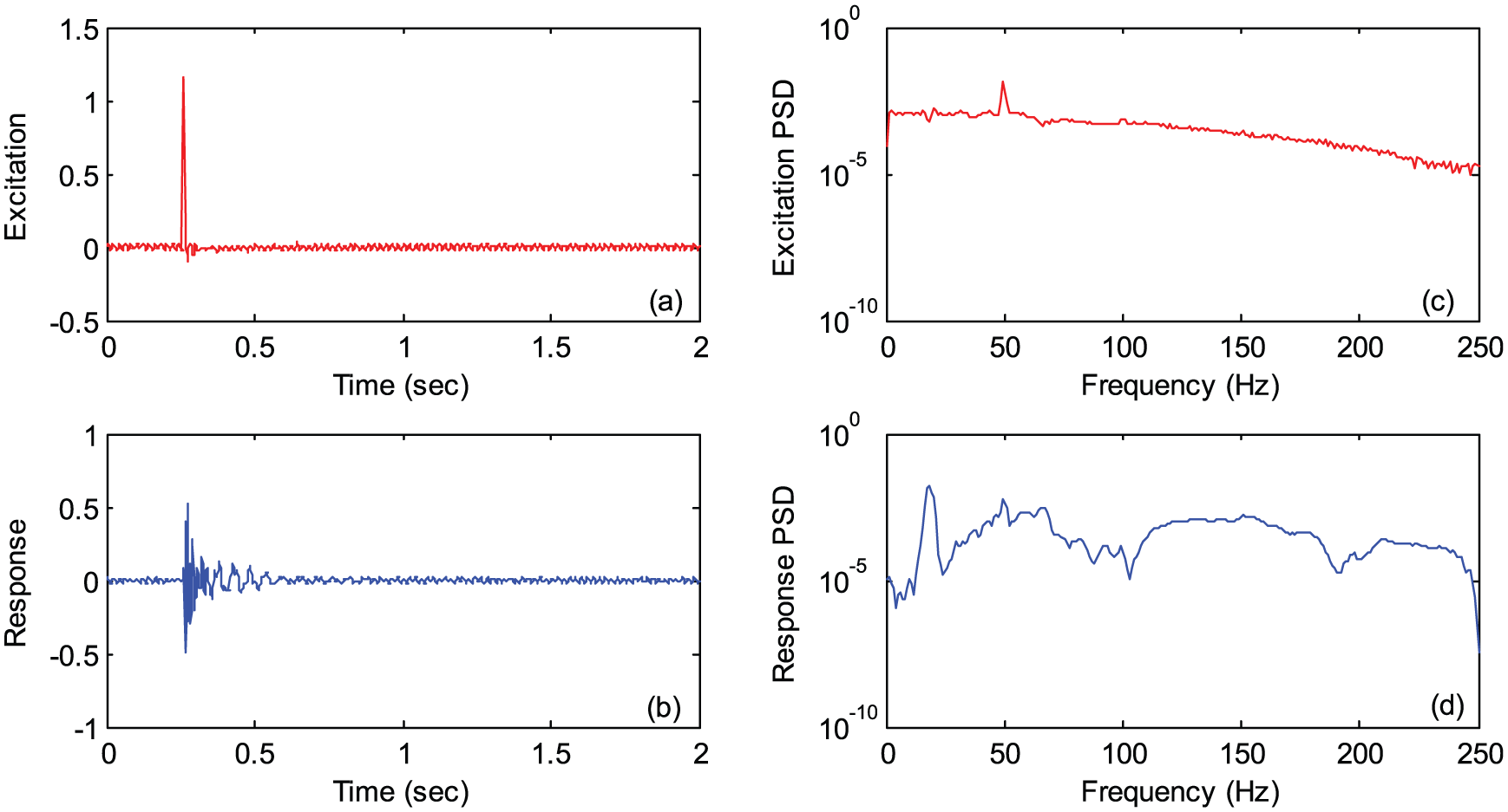
Example of (a) excitation time-series, (b) excitation power spectrum densities, (c) response time-series and (d) response power spectrum densities recorded during the modal test.

Data acquisition was conducted using a 48-channel signal conditioning box that amplified the signals to the range of ±10 V. This equipment was connected to a 16-bit Analog Data Acquisition and Control Cube (United Electronics DNA-PPC5). The system was controlled by a MATLAB code developed by the authors. A fifth-order Butterworth low-pass filter was applied, with a 200-Hz cut-off frequency.

SSI (Van Overschee and De Moor, 1996) was used for extracting the modal properties from the recorded data. The SSI approach is a data-driven time-domain technique that employs QR-factorization and singular value decomposition to identify the matrices of the dynamic state-space model. Once the state-space model of the structure is found, the modal parameters (natural frequencies, damping ratios and mode shapes) can be determined by eigenvalue decomposition. This kind of system identification method has been successfully applied for extracting modal properties of structures excited by impacts and other kinds of broadband excitation (Altunisik et al., 2012; Osmancikli et al., 2012; Ramos et al., 2010a; Reynders et al., 2010; Reynders and Roeck, 2008). The SSI algorithm was applied to every independent impact test, with 18 tests per wall (72 tests in total). In each case, the SSI analysis was conducted considering a Hankel’s matrix row size equal to 30 and a maximum system order (SO_max) equal to 100 or 70 depending on the instrumental setup employed in each case.

Vibration-based damage indentificators

The relationship observed between degradation of structural properties (stiffness and mass) and changes in modal frequencies was a main promoter for developing vibration-based damage identification techniques. Because frequency measurements can be quickly conducted and have a lower data scatter than do mode shapes and damping measurements, damage parameters related to modal frequencies have historically been preferred (Salawu, 1997). In the study presented here, statistically significant variations of the modal frequencies (measured before and after damage) were employed to detect structural degradation. Our frequency-based analysis was conducted considering that the recorded frequencies were normally distributed. Hypothesis tests considering a 95% confidence were applied to determine whether corresponding frequencies detected at different states of damage were statistically different or similar. Statistically significant differences were assumed as a potential evidence of damage.

Another damage indicator considers changes in mode shapes detected before and after damage was generated. The difference in mode shapes can be originated by stiffness degradation, change in the mass distribution and alterations in the system boundary/connectivity conditions. The MAC is an indicator that quantifies the degree of similarity between two mode shape vectors (equation (1)) and is therefore used to detect differences between mode shapes measured before and after damage. Previous studies (Doebling et al., 1996) have confirmed that a good result can be achieved, even in the case when frequency-based indicators were not able to identify structural deterioration. The equation that defines MAC is

MA C_{j} = \frac{{({ϕ_{j}^{0}}^{T} \cdot {ϕ_{j}^{D}})}^{2}}{({ϕ_{j}^{0}}^{T} \cdot {ϕ_{j}^{0}}) \cdot ({ϕ_{j}^{D}}^{T} \cdot {ϕ_{j}^{D}})}

(1)

where ${ϕ_{j}^{0}}$ and ${ϕ_{j}^{D}}$ correspond to the mode shape vectors of the jth mode for the undamaged and damaged condition, respectively. In the study presented here, whenever mode shape information was available for two damage states in the same wall, the MAC value was computed and the average value of the calculated MAC was considered as a damage indicator.

The effectiveness of the above introduced indicators to identify damage in URM structures under ideal conditions (e.g. homogeneous properties of bricks and mortar and perfect connection at the brick–mortar interface) was successfully demonstrated in preliminary tests using numerical simulations and in physical tests on simple URM structures (Oyarzo-Vera and Chouw, 2013). This study verified that MAC is more effective for advanced levels of damage, when not only the global stiffness of the structure is affected but also the boundary conditions or internal connections are modified due to cracking or similar kind of damage.

Results

Observed damage

The first excitation sequence (ES1) produced no visible damage (DS1). However, an excessive and undesired vertical deformation was observed in the diaphragm. This deformation originated in an overturning moment by the shaker, which produced a detachment of the floor boards and plywood sheets from the joists. This detachment affected the transference of load from the shaker, through the diaphragm, to the walls. To prevent this floor detachment, two box-section steel joists were added to the diaphragm in the north–south direction. These members were placed at the top of the diaphragm and firmly bolted to the timber joists below the diaphragm. The addition of the steel joists significantly reduced the vertical deformation of the diaphragm during the second excitation sequence (ES2), but did not eliminate that deformation completely.

As no visible damage was observed at DS2, it was decided to increase the magnitude and duration of the next excitation sequence (ES3) to 10.4 kN and 180 s, respectively. As expected, significant and visible damage was generated in the specimen (DS3). In the south wall, a long horizontal crack at the diaphragm level was observed (Figure 5(a)) and diagonal cracks around the door opening were detected in the north wall. Also, several cracks were detected at the upper corners of the walls. These cracks were related to out-of-plane failure of the parapet (Figure 5(b) and (c)).

Figure 5.

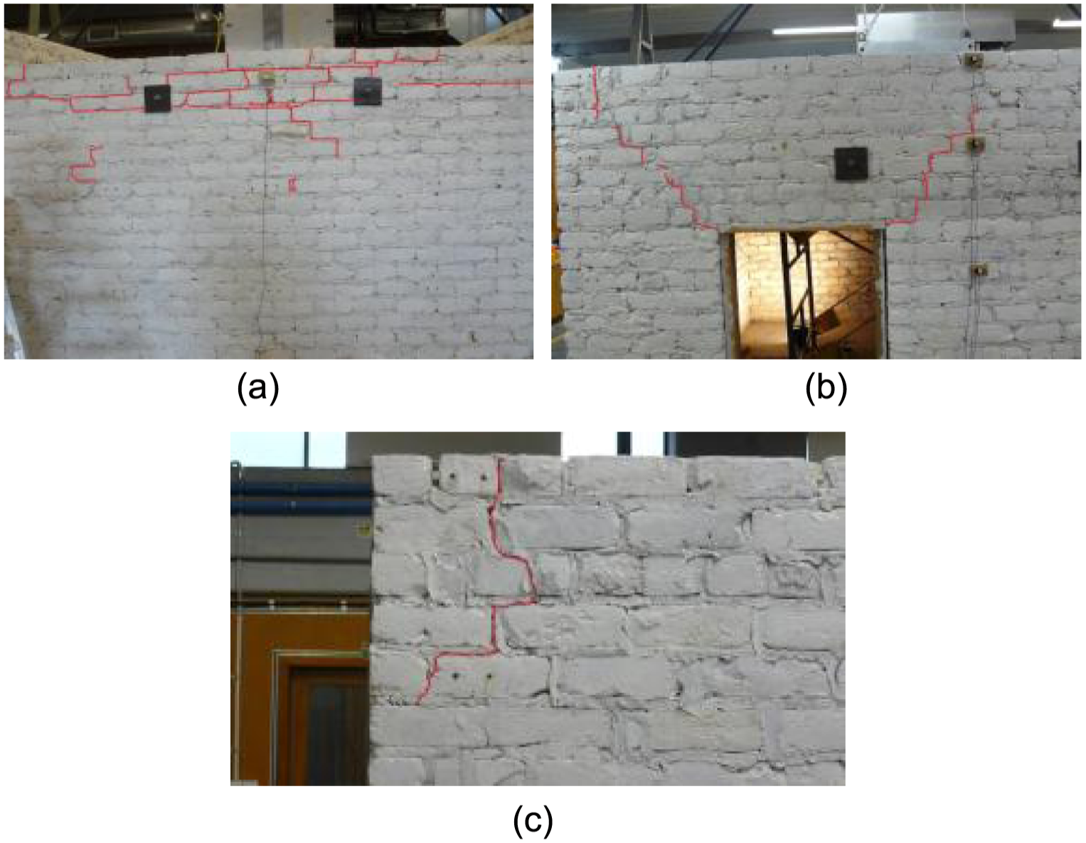
Damage observed at DS3: (a) south wall, (b) north wall and (c) north-west walls’ corner.

The final excitation sequence (ES4) produced severe damage, especially in the north and south walls (DS4). In the south wall, the two upper brick courses fell down and diagonal cracks typical of wall out-of-plane failure were developed (Figure 6(a)). The parapet of the north wall was heavily damaged, even losing some bricks. The cracks around the door and window openings that had been previously detected now became wider and new cracks were also identified (Figure 6(b)). Cracks were noticed around the window openings of the east and west walls, but the most significant damage was observed in the upper corners of those walls, probably because of the effect of the out-of-plane failure of the north and south walls (Figure 6(c) and (d)).

Figure 6.

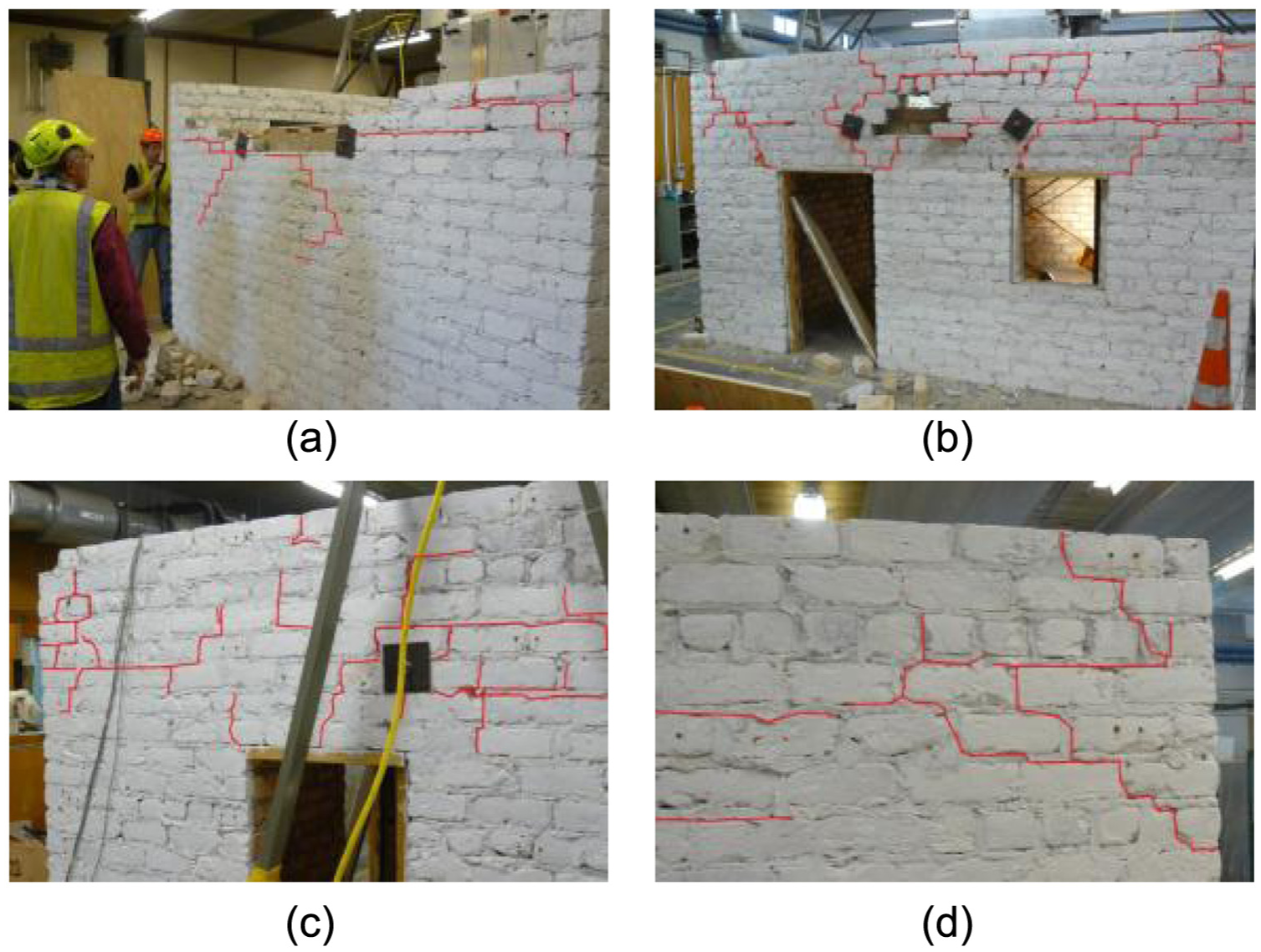
Damage observed at DS4: (a) south wall, (b) north wall, (c) north-west walls’ corner and (d) south-west walls’ corner.

As expected, the walls most severely affected were those experiencing the excitation normal to their plane (north and south walls). The walls that work as the primary resistant system (east and west walls) only experienced localized damage due to excessive out-of-plane displacement of the other walls. These observations support the initial decision of only measuring the out-of-plane response of walls during the modal tests.

Modal properties and damage identification

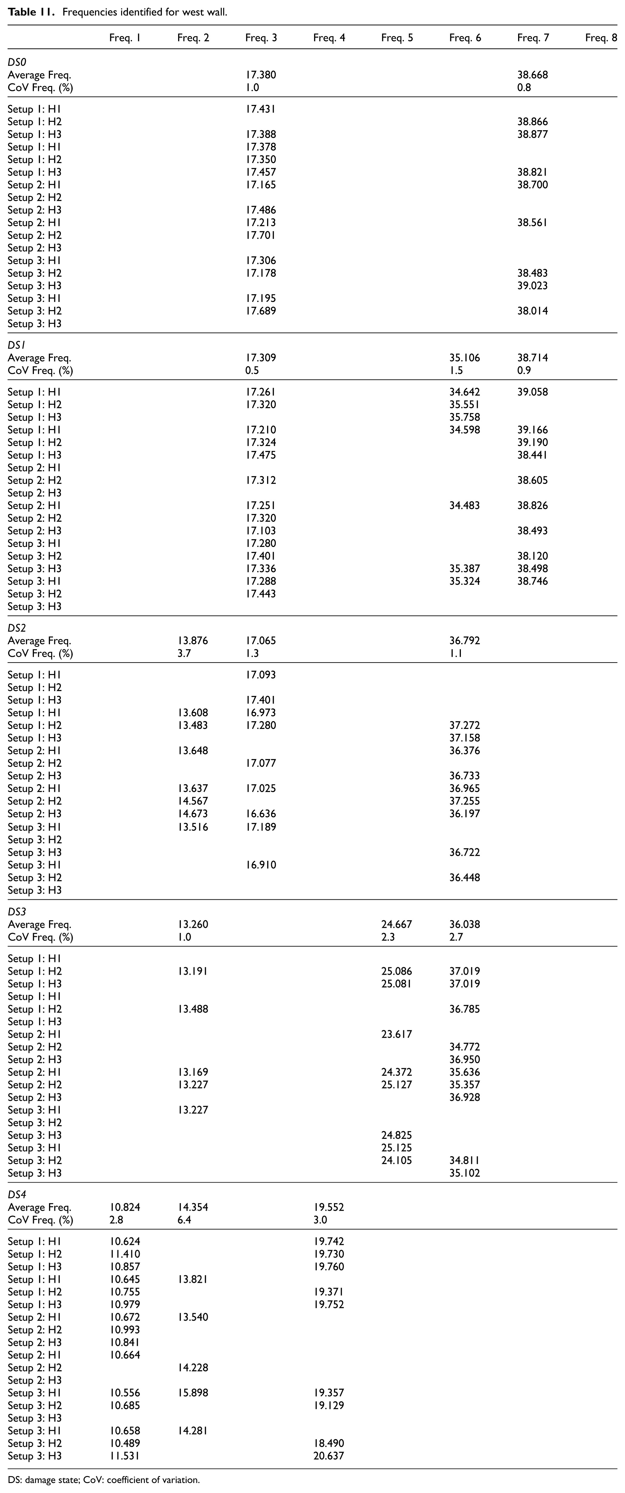
The modal frequencies identified by the SSI method are shown in Table 2. The complete record of identified frequencies has been included in Appendix 1. It must be noted the low dispersion of the frequencies identified for each mode (coefficient of variation (CoV) ≤ 5% in almost all cases). It was observed that different modes were generally related to the response of specific parts of the building (walls or diaphragm response). Nevertheless, there were several frequencies detected in multiple walls that were associated with a global system response or corresponded to the response of other parts of the structure indirectly excited by the impact. In the case of DS4, no information is presented for the north and south walls because the response was not measured in those walls due to their severe deterioration at this state of damage.

Table 2.

Modal frequencies (Hz) detected in the specimen.

	Wall	DS0	DS1	DS2	DS3	DS4
		Average (CoV)	Average (CoV)	Average (CoV)	Average (CoV)	Average (CoV)
Freq. 1	North				11.875 (5%)	−
	South				11.600 (5%)	−
	East					10.664 (3%)
	West					10.824 (3%)
Freq. 2	North					−
	South					−
	East			13.602 (2%)	13.645 (3%)	12.265 (8%)
	West			13.876 (4%)	13.260 (1%)	14.354 (6%)
Freq. 3	North	18.250 (1%)	17.203 (3%)			−
	South	17.598 (1%)	16.857 (2%)	16.906 (2%)	16.670 (3%)	−
	East	17.536 (1%)	17.222 (2%)	17.640 (4%)	16.867 (5%)
	West	17.380 (1%)	17.309 (1%)	17.065 (1%)	16.189 (1%)
Freq. 4	North	20.953 (1%)	19.767 (2%)	20.267 (3%)		−
	South	19.203 (2%)	19.244 (3%)			−
	East					19.668 (3%)
	West					19.552 (3%)
Freq. 5	North				24.657 (4%)	−
	South					−
	East			25.792 (1%)	25.092 (1%)	25.050 (1%)
	West				24.667 (2%)
Freq. 6	North	36.623 (1%)	36.251 (2%)			−
	South					−
	East		36.066 (1%)	37.098 (1%)	37.278 (1%)
	West		35.106 (1%)	36.792 (1%)	36.038 (3%)
Freq. 7	North	38.878 (1%)				−
	South			38.987 (1%)	38.285 (2%)	−
	East
	West	38.668 (1%)	38.714 (1%)
Freq. 8	North			41.203 (1%)	40.491 (2%)	−
	South		40.611 (2%)			−
	East	39.995 (1%)	39.558 (1%)		39.248 (1%)
	West

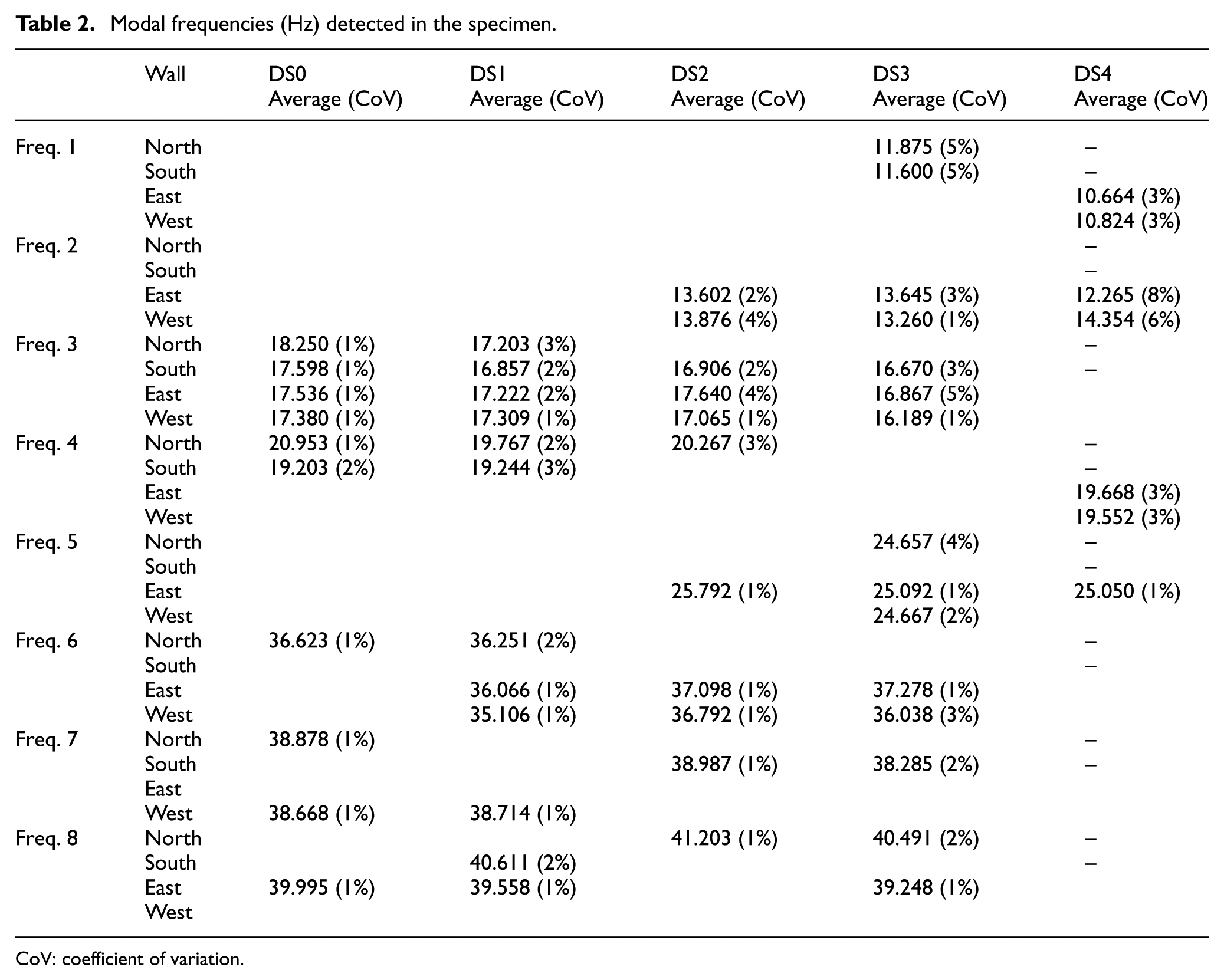
CoV: coefficient of variation.

For damage identification, three study cases were analysed: (1) structural dynamic behaviour before reinforcing the diaphragm with steel joists (Case 1: DS0 compared to DS1), (2) the effect of diaphragm reinforcement on the dynamic behaviour (Case 2: DS1 compared to DS2) and (3) the effect of damage on the dynamic behaviour of the structure with the reinforced diaphragm (Case 3: DS3 and DS4 compared to DS2). In each of these cases, only those modes detected in the reference damage state and in at least one of the subsequent damage states were considered. Those modes that were not detected in the reference damage state (new modes generated by damage or structural modification) were omitted in this analysis. The response of every wall was considered independently. The average MAC values were calculated considering the mode shape information available for each damage state as it is presented between parentheses in Table 3.

Table 3.

Mode pairs considered in each analysis case to compute MAC.

	North wall	South wall	East wall	West wall
Case 1: DS0-DS1	Freq. 3 (87%)Freq. 4 (94%)	Freq. 4 (96%)	Freq. 3 (95%)	Freq. 3 (95%)
Case 2: DS1-DS2	Freq. 4 (92%)		Freq. 3 (94%)	Freq. 3 (96%)
Case 3a: DS2-DS3	Freq. 8 (8%)	Freq. 3 (83%)	Freq. 2 (83%)Freq. 3 (54%)	Freq. 2 (57%)Freq. 3 (93%)Freq. 6 (41%)
Case 3b: DS2-DS4			Freq. 2 (9%)Freq. 5 (13%)	Freq. 2 (75%)

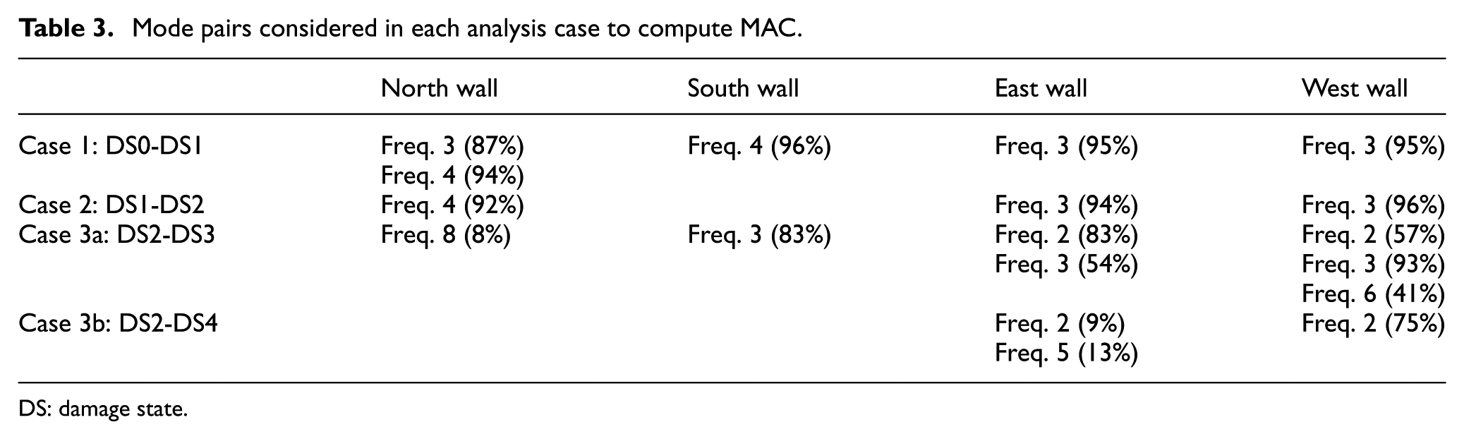
DS: damage state.

Case 1: structural dynamic behaviour before reinforcing the diaphragm

Recognizing that no evident damage was observed in the structure due to the first excitation sequence (ES1), it would be expected that no major difference in building condition should be detected between the results of DS0 and DS1. This situation was reflected in the results presented in Table 2 for DS0 and DS1, where the same set of modal frequencies was detected in both damage states. Nevertheless, minor system alterations might be anticipated, because of an incipient non-visible damage, especially considering the pristine condition of the structure at DS0. It can be expected that the diaphragm detachment due to the shaker overturning moment observed during ES1 might affect the modal response of the structure, for example, by a generalized stiffness degradation or changes in the connectivity conditions between walls and diaphragm.

The modal frequency labelled as Freq. 3 was clearly identified in all walls at approximately 17 Hz. Considering the results obtained from numerical models (Oyarzo-Vera, 2012) and the response recorded at higher levels of damage (DS3 and DS4), it was assumed that Freq. 3 was related to a modal response with an important participation of the south wall. This is also consistent with the fact that south wall was thinner (110 mm) and, therefore, it was easier to excite due to its relatively smaller stiffness.

Freq. 4 was detected at approximately 20 Hz. This mode was related to a north–south response of the structure with a significant participation of the north wall. The inclusion of wall-diaphragm connectors contributed to a transfer of the response of north wall, through the diaphragm, to the south wall. Freq. 6 was related to another mode with a significant participation of the north wall (at approximately 36 Hz) which was also detected in the east and west walls.

Freq. 7 and Freq. 8 corresponded to twin modes associated with the west and east walls, respectively. Under ideal conditions, the frequency and mode shapes of these twin modes would be completely identical. The difference observed between these modes was attributed to potential dissimilarities in material properties, support conditions and construction quality.

In terms of damage identification, statistically significant frequency reduction was observed in several modes (labelled with a ‘Y’ in Table 4), especially in the walls that had the most important participation in the corresponding mode. The most significant frequency reductions for Freq. 3 and Freq. 4 occurred in the south and north walls, respectively. A significant frequency drop was also detected in Freq. 8 associated with a mode principally recorded in the east wall. This observed frequency degradation was explained by a general degradation (softening) of materials that did not necessarily manifest itself as visible cracks. This general degradation in stiffness did not affect particular part of the structure or alter the wall boundary conditions. Therefore, the relative magnitudes of modal displacements within the mode shape vectors measured before and after damage were not altered, as can be inferred from the relatively high MAC values computed for this case (Figure 7 and Table 2, Case 1).

Table 4.

Modal frequency variation before reinforcing the diaphragm (Case 1: DS1 vs DS0).

	Wall	DS0	DS1
		Ref. Freq.	Freq. Var. (%)	Sig. Var.
Freq. 3	North	18.250	−5.7	No
	South	17.598	−4.2	Yes
	East	17.536	−1.8	Yes
	West	17.380	−0.4	No
Freq. 4	North	20.953	−5.7	Yes
	South	19.203	0.2	No
	East
	West
Freq. 6	North	36.623	−1.0	No
	South
	East
	West
Freq. 7	North
	South
	East
	West	38.668	0.1	No
Freq. 8	North
	South
	East	39.995	−1.1%	Yes
	West

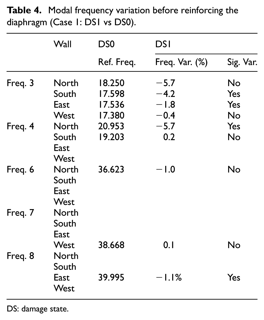
DS: damage state.

Figure 7.

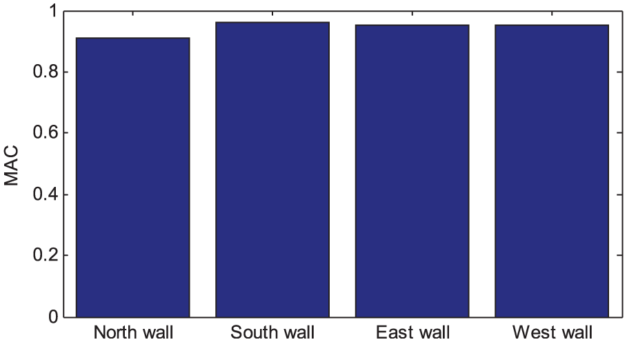
MAC obtained for Case 1 (DS1 compared to the reference DS0).

Case 2: effect of the diaphragm reinforcement on the dynamic behaviour

As described previously, two steel joists were used to reinforce the diaphragm after DS1 with the aim of reducing the vertical deformation due to the overturning moment generated by the shaker. This intervention in the structure was considered as a retrofit that altered the system baseline conditions. To conduct the most appropriate analysis, DS2 was considered as a reference condition for examination of the subsequent states of damage. The reference state DS2 considered a system configuration that included the diaphragm reinforcement and a relatively low level of damage generated by the low magnitude excitation sequences ES1 and ES2. This new configuration contributed to the generation of a new set of modal frequencies associated with the new reference condition DS2 (Table 2).

Freq. 2 corresponded to a mode at approximately 13 Hz, mainly associated with a response of the east and west walls. That mode was not detected in the previous damage states before reinforcing the diaphragm.

Freq. 3 was detected for DS2 at 17 Hz. This mode was also detected at DS0 and DS1 and was associated with the south wall response. In the case of DS2, the relation between this mode and the south wall was confirmed. The mode was also identified at DS3, but at a slightly lower frequency (16.6 Hz).

Freq. 4 was detected in the north wall at 20 Hz, similar to the results obtained for DS0 and DS1. This frequency disappeared in the subsequent states of damage (DS3 and DS4). For DS4, a frequency of approximately 19.5 Hz was detected in the east and west walls, but the correspondence of that frequency to the mode previously detected in the north wall was not completely clear.

Freq. 5 was not identified in DS0 and DS1, but was clearly detected in DS2 and the subsequent states of damage. This mode had a frequency of approximately 24 Hz and was related to a modal response dominated by east wall vibration.

Freq. 6, of approximately 36.5 Hz, was related to a modal response of the east and west walls. In the previous states of damage, this frequency was related to a mode with a predominant participation of the north wall.

Freq. 7 and Freq. 8 (of approximately 38.5 and 40 Hz, respectively) were related to modal responses with strong participation of the south and north walls, respectively.

One of the effects generated by the diaphragm reinforcement corresponds to a change in the modes order. Before the diaphragm was reinforced, Freq. 7 and Freq. 8 were twin frequencies (around 39 Hz) related to a response dominated by vibration of the west and east walls. After retrofit, these modes became indistinguishable and appeared together at 37 Hz as Freq. 6, while Freq. 7 and Freq. 8 turned into modes related to south and north walls, respectively.

All the changes observed in the modal frequencies were generated by the structural degradation due to low-intensity applied loads (ES1 and ES2) and the diaphragm reinforcement. This supports the decision of considering DS2 as reference condition in all the subsequent analysis because the original baseline (DS0) was no longer valid.

In terms of damage identification, statistically significant increments of the modal frequencies were observed in Freq. 4 and Freq. 6 (labelled with a ‘Y’ in Table 5). This frequency rise was related to a restitution of stiffness and structural integrity due to reinforcement of the diaphragm. An exception to this behaviour was observed in the west wall for Freq. 3, in which modal frequency dropped. However, participation of the west wall was secondary in this mode.

Table 5.

Effect of the diaphragm reinforcement in the modal frequencies (Case 2: DS2 vs DS1).

	Wall	DS1	DS2
		Ref. Freq.	Freq. Var. (%)	Sig. Var.
Freq. 3	North
	South	16.857	0.3	No
	East	17.222	2.4	No
	West	17.309	−1.4	Yes
Freq. 4	North	19.767	2.5	Yes
	South
	East
	West
Freq. 6	North
	South
	East	36.066	2.9	Yes
	West	35.106	4.8	Yes

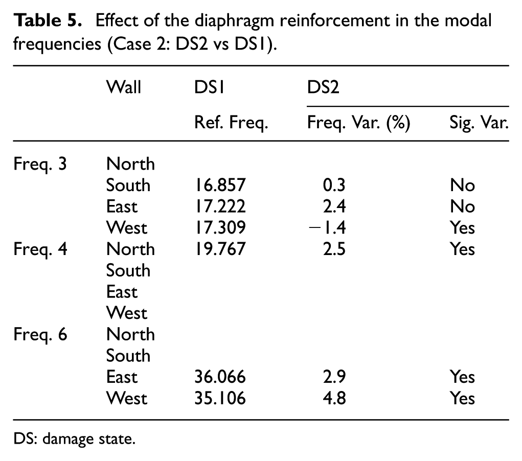
DS: damage state.

Similar to the situation observed in the previous study case, the MAC values computed for each wall were high (Figure 8 and Table 2, Case 2). The high MAC values showed an elevated level of correspondence between the mode shapes of DS1 and DS2, probably because no damage was produced in the walls to generate a variation in the relative magnitudes of the modal displacements within the mode shape vectors. Unfortunately, it was not possible to obtain reliable results of MAC in the south wall.

Figure 8.

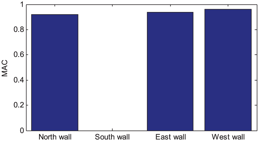
MAC obtained for Case 2 (DS2 compared to the reference DS1).

Case 3: structural dynamic behaviour after reinforcing the diaphragm

The third case of analysis considers the effect of the large magnitude excitation (ES3 and ES4) having as reference the dynamic behaviour recorded at DS2. One of the most evident effects of severe damage of the structure was the detection of another low frequency mode at approximately 11 Hz (Freq. 1 in Table 2). This mode was interpreted as a result of cantilever vibration of the parapets. These structural elements lost their lateral supports due to damage in the wall corners and they became independent cantilever panels. Hence, parapets responded at different resonant frequencies than those recorded before damage. However, this interpretation was only intuitive and no sufficient data were available to confirm this hypothesis.

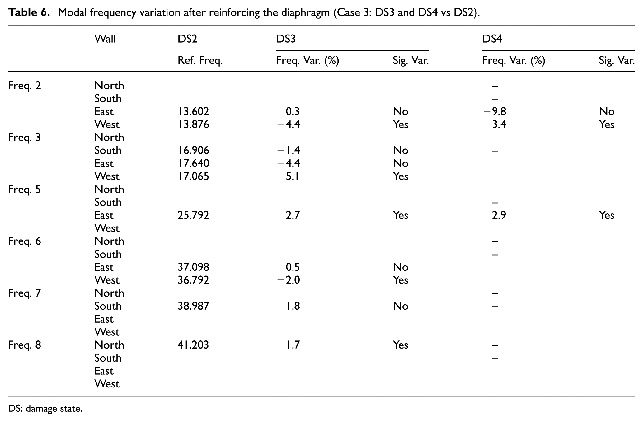
In terms of damage indicators, the large magnitude load sequences (ES3 and ES4) produced a significant reduction in most of the modal frequencies (Table 6), except for Freq. 7. It is noted that Freq. 2 and Freq. 5 corresponded to modes detected after the inclusion of the steel joists used to reinforce the diaphragm. For the case of DS3 compared to DS2 (Figure 9(a) and Table 2, Case 3a), damage was also detected by the MAC in all the walls (MAC <85%), with the effect being more accentuated in the north wall which coincided with the severe damage observed in the experiment. A less significant difference was observed in the south wall, which was explained by the damage concentrated at the top of the wall and almost insignificant damage in the rest of the panel. The differences observed in the east and west walls were attributable to indirect effects of the damage in the north and south walls. The MAC factors calculated for the case of DS4 compared to DS2 (Figure 9(b) and Table 2, Case 3b) were also affected by damage; however, the results were not totally consistent with the damage progression. MAC decreased in the east wall, while it increased in the west wall. It is important to remember that no measurements were performed in the north and south walls at DS4 due to the excessive damage generated. Therefore, frequencies and MAC cannot be determined in these walls for this damage state.

Table 6.

Modal frequency variation after reinforcing the diaphragm (Case 3: DS3 and DS4 vs DS2).

	Wall	DS2	DS3		DS4
		Ref. Freq.	Freq. Var. (%)	Sig. Var.	Freq. Var. (%)	Sig. Var.
Freq. 2	North				−
	South				−
	East	13.602	0.3	No	−9.8	No
	West	13.876	−4.4	Yes	3.4	Yes
Freq. 3	North				−
	South	16.906	−1.4	No	−
	East	17.640	−4.4	No
	West	17.065	−5.1	Yes
Freq. 5	North				−
	South				−
	East	25.792	−2.7	Yes	−2.9	Yes
	West
Freq. 6	North				−
	South				−
	East	37.098	0.5	No
	West	36.792	−2.0	Yes
Freq. 7	North				−
	South	38.987	−1.8	No	−
	East
	West
Freq. 8	North	41.203	−1.7	Yes	−
	South				−
	East
	West

DS: damage state.

Figure 9.

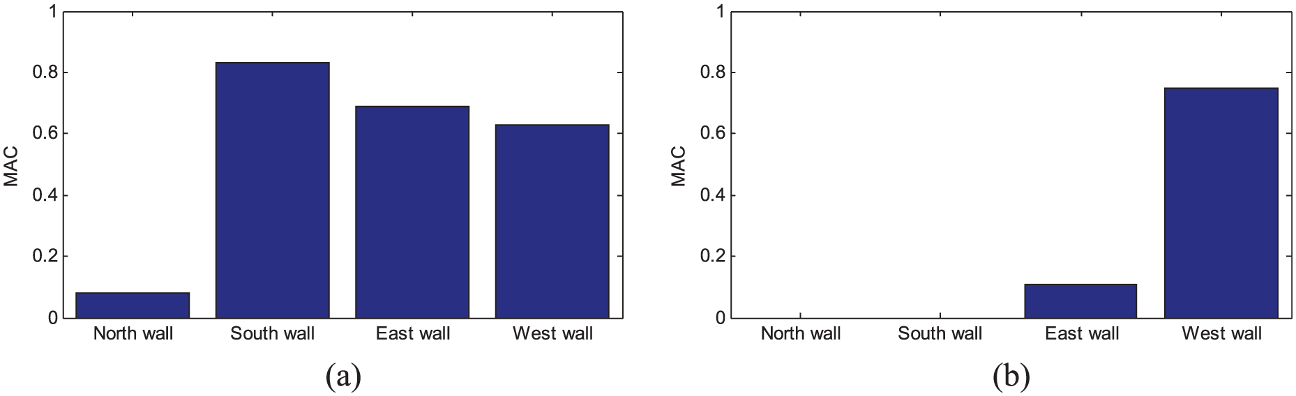
MAC obtained for Case 3: (a) DS3 compared to the reference DS2 and (b) DS4 compared to the reference DS2.

Damage history

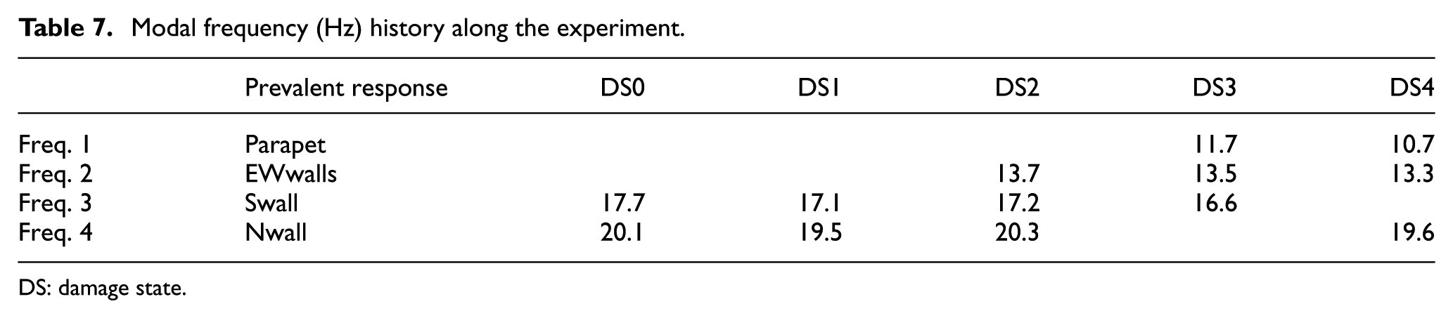
The global behaviour of the structure is presented in Table 7 in terms of the average value of the frequencies recorded in the different walls. Only the first 4 modes were considered in this analysis because their evolution was easier to follow along the entire experiment history. The second column in Table 7 specifies the prevalent response associated with each frequency. Frequency variations and MAC values computed for each of the vibration modes at different states of damage are shown in Figure 10. In all the cases, the mode detected at the earliest damage state was used as reference and that reference frequency and MAC were defined as one. In some cases, it was not possible to calculate MAC because frequencies were detected in different walls and mode shapes were not comparable.

Table 7.

Modal frequency (Hz) history along the experiment.

	Prevalent response	DS0	DS1	DS2	DS3	DS4
Freq. 1	Parapet				11.7	10.7
Freq. 2	EWwalls			13.7	13.5	13.3
Freq. 3	Swall	17.7	17.1	17.2	16.6
Freq. 4	Nwall	20.1	19.5	20.3		19.6

DS: damage state.

Figure 10.

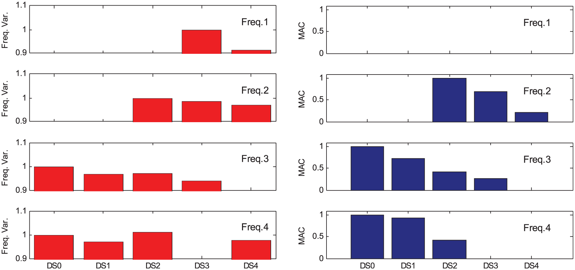
Global frequency and global MAC evolution during the experiment.

It can be observed that Freq. 1, associated to parapet’s vibrations, decayed which was interpreted as an evidence of the progressive loss of lateral support of parapets. Freq. 2 also decayed with damage and it can be interpreted as a global stiffness degradation of the structure in the EW direction. In the case of Freq. 3, it decreased after the first excitation sequence (DS1), stayed constant after the second excitation sequence (DS2) and dropped significantly due to the strong excitation sequence (DS3). This situation was related to the sustained damaging of the south wall that affects the entire modal response of the structure. Something similar occurred with Freq. 4 associated to north wall response. In both cases (Freq. 3 and Freq. 4), it is important to note that frequency changes were observed although no visible damage was detected. Hence, this parameter was able to detect early stages of damage. However, the severity of damage is still no quantifiable by this indicator.

MAC was even more consistent than frequency variations. It decayed persistently with the increase in damage along the entire experiment history. The same as in frequency, MAC changes were not necessarily proportional to damage severity.

Conclusion

The results of an experimental study of an URM house model were presented. The house was dynamically loaded using eccentric-mass shakers placed on the roof, and structural damage to the walls was initiated by increasing the amplitude of the applied load. At each damage state, a modal test was performed by impacting the house using a calibrated hammer. The dynamic properties of the structure at the considered damage states were extracted from the recorded accelerations by SSI techniques. Finally, vibration-based damage identification procedures were applied to detect and determine the spatial distribution of damage in the structure. Two damage indicators were considered in this analysis: (1) significant variation of modal frequencies and (2) MAC.

The results obtained from the system identification analysis revealed different sets of modes for different states of damage. New modes were detected while other modes vanished along the course of the test. The appearance and disappearance of modes were caused by the combination of several phenomena, such as material degradation, change in the support and boundary/connectivity conditions, and breaks in the continuity of the members (cracks), all due to the damage induced by excitation sequences. Also, the system alterations produced by the retrofit applied to the diaphragm after DS1 could be another explanation of that phenomenon.

None of the low magnitude excitation sequences (ES1 and ES2) generated visible damage. However, a decrement of the most predominant frequencies (Freq. 3) was observed in all walls, which was attributed to a generalized degradation of stiffness (material softening). The detection of such system alterations at early states of damage was considered an advantage of the method because changes in this modal frequency might potentially be used as a damage indicator. Unfortunately, although the frequency drop observed in Freq. 3 persisted in the subsequent states of damage (DS3 and DS4), it was not always statistically significant.

The large magnitude excitations (ES3 and ES4) produced statistically significant frequency drops in most modes. Nevertheless, the magnitude of the frequency variation was not always consistent with the severity of the damage observed. The most significant frequency variations were not associated with the most severely damaged walls.

A reduction in the MAC value was observed only when severe damage was generated (DS3 and DS4). When the damage was not manifested as cracks or any other phenomena that altered the mode shapes geometry (e.g. change in boundary conditions), MAC was unable to detect damage (DS0 vs DS1 and DS1 vs DS2).

The relative severity of damage was not properly reflected by MAC. More severely damaged walls (e.g. the south wall) did not necessarily exhibit a smaller MAC than that of other walls that had experienced a milder damage (e.g. the east and west walls). Consequently, MAC can be used to detect severe damage, but it is ineffective for comparing the relative damage generated in each of the walls.

Finally, for determining the spatial distribution damage, it was necessary to realize how the different modes were related to the response of different parts of the specimen. Based on the information collected for the individual walls, a rough identification of the spatial distribution of damage (the determination of which wall is damaged) can be achieved with acceptable levels of reliability. This kind of information would allow analysts to identify parts of the building that need to be modified to represent damage instead of modifying a global property, for example, in a finite element model. This would recognize the localized nature of damage.

Footnotes

Appendix 1

Table 11.

Frequencies identified for west wall.

	Freq. 1	Freq. 2	Freq. 3	Freq. 4	Freq. 5	Freq. 6	Freq. 7
DS0
Average Freq.			17.380				38.668
CoV Freq. (%)			1.0				0.8

Setup 1: H1			17.431
Setup 1: H2							38.866
Setup 1: H3			17.388				38.877
Setup 1: H1			17.378
Setup 1: H2			17.350
Setup 1: H3			17.457				38.821
Setup 2: H1			17.165				38.700
Setup 2: H2
Setup 2: H3			17.486
Setup 2: H1			17.213				38.561
Setup 2: H2			17.701
Setup 2: H3
Setup 3: H1			17.306
Setup 3: H2			17.178				38.483
Setup 3: H3							39.023
Setup 3: H1			17.195
Setup 3: H2			17.689				38.014
Setup 3: H3

DS1
Average Freq.			17.309			35.106	38.714
CoV Freq. (%)			0.5			1.5	0.9

Setup 1: H1			17.261			34.642	39.058
Setup 1: H2			17.320			35.551
Setup 1: H3						35.758
Setup 1: H1			17.210			34.598	39.166
Setup 1: H2			17.324				39.190
Setup 1: H3			17.475				38.441
Setup 2: H1
Setup 2: H2			17.312				38.605
Setup 2: H3
Setup 2: H1			17.251			34.483	38.826
Setup 2: H2			17.320
Setup 2: H3			17.103				38.493
Setup 3: H1			17.280
Setup 3: H2			17.401				38.120
Setup 3: H3			17.336			35.387	38.498
Setup 3: H1			17.288			35.324	38.746
Setup 3: H2			17.443
Setup 3: H3

DS2
Average Freq.		13.876	17.065			36.792
CoV Freq. (%)		3.7	1.3			1.1

Setup 1: H1			17.093
Setup 1: H2
Setup 1: H3			17.401
Setup 1: H1		13.608	16.973
Setup 1: H2		13.483	17.280			37.272
Setup 1: H3						37.158
Setup 2: H1		13.648				36.376
Setup 2: H2			17.077
Setup 2: H3						36.733
Setup 2: H1		13.637	17.025			36.965
Setup 2: H2		14.567				37.255
Setup 2: H3		14.673	16.636			36.197
Setup 3: H1		13.516	17.189
Setup 3: H2
Setup 3: H3						36.722
Setup 3: H1			16.910
Setup 3: H2						36.448
Setup 3: H3

DS3
Average Freq.		13.260			24.667	36.038
CoV Freq. (%)		1.0			2.3	2.7

Setup 1: H1
Setup 1: H2		13.191			25.086	37.019
Setup 1: H3					25.081	37.019
Setup 1: H1
Setup 1: H2		13.488				36.785
Setup 1: H3
Setup 2: H1					23.617
Setup 2: H2						34.772
Setup 2: H3						36.950
Setup 2: H1		13.169			24.372	35.636
Setup 2: H2		13.227			25.127	35.357
Setup 2: H3						36.928
Setup 3: H1		13.227
Setup 3: H2
Setup 3: H3					24.825
Setup 3: H1					25.125
Setup 3: H2					24.105	34.811
Setup 3: H3						35.102

DS4
Average Freq.	10.824	14.354		19.552
CoV Freq. (%)	2.8	6.4		3.0

Setup 1: H1	10.624			19.742
Setup 1: H2	11.410			19.730
Setup 1: H3	10.857			19.760
Setup 1: H1	10.645	13.821
Setup 1: H2	10.755			19.371
Setup 1: H3	10.979			19.752
Setup 2: H1	10.672	13.540
Setup 2: H2	10.993
Setup 2: H3	10.841
Setup 2: H1	10.664
Setup 2: H2		14.228
Setup 2: H3
Setup 3: H1	10.556	15.898		19.357
Setup 3: H2	10.685			19.129
Setup 3: H3
Setup 3: H1	10.658	14.281
Setup 3: H2	10.489			18.490
Setup 3: H3	11.531			20.637

DS: damage state; CoV: coefficient of variation.

Declaration of Conflicting Interests

The author(s) declared no potential conflicts of interest with respect to the research, authorship and/or publication of this article.

Funding

The author(s) disclosed receipt of the following financial support for the research, authorship and/or publication of this article: The authors acknowledge the support of the New Zealand Foundation for Research, Science and Technology (Project UOAX0411) for this research program, and the support of the Chilean Government (Beca Presidente de la República) and the Universidad Católica de la Santísima Concepción (UCSC, Chile) that enabled the first author’s doctoral studies in New Zealand.

References

Altunisik

Bayraktar

Sevim

(2012) Operational modal analysis of a scaled bridge model using EFDD and SSI methods. Indian Journal of Engineering and Materials Sciences 19(5): 320–330.

ASTM C270 (2008) Standard Specification for Mortar for Unit Masonry. West Conshohocken, PA: ASTM International.

ASTM C1314 (2010) Standard Test Method for Compressive Strength of Masonry Prisms. West Conshohocken, PA: ASTM International.

Beyen

(2008) Structural identification for post-earthquake safety analysis of the Fatih mosque after the 17 August 1999 Kocaeli earthquake. Engineering Structures 30(8): 2165–2184.

Ceroni

Sica

Pecce

. (2014) Evaluation of the natural vibration frequencies of a historical masonry building accounting for SSI. Soil Dynamics and Earthquake Engineering 64: 95–101.

Dizhur

Ingham

(2013) Diagonal tension strength of vintage unreinforced clay brick masonry wall panels. Construction & Building Materials 43: 418–427.

Doebling

Farrar

Prime

. (1996) Damage Identification and Health Monitoring of Structural and Mechanical Systems from Changes in their Vibration Characteristics: A Literature Review (LA-13070-MS). Los Alamos, NM: Los Alamos National Laboratory.

Durukal

Cimilli

Erdik

(2003) Dynamic response of two historical monuments in Istanbul deduced from the recordings of Kocaeli and Duzce earthquakes. Bulletin of the Seismological Society of America 93(2): 694–712.

Farrar

Worden

(2007) An introduction to structural health monitoring. Philosophical Transactions of the Royal Society A: Mathematical, Physical and Engineering Sciences 365: 303–315.

10.

Gentile

Saisi

(2007) Ambient vibration testing of historic masonry towers for structural identification and damage assessment. Construction and Building Materials 21(6): 1311–1321.

11.

Lumantarna

Biggs

Ingham

(2014) Uniaxial compressive strength and stiffness of field extracted and laboratory constructed masonry prisms. Journal of Materials in Civil Engineering: ASCE 26(4): 567–575.

12.

Moon

Dizhur

Senaldi

. (2014) The demise of the URM building stock in Christchurch during the 2010/2011 Canterbury earthquake sequence. Earthquake Spectra 30(1): 253–276.

13.

Osmancikli

Ucak

Turan

. (2012) Investigation of restoration effects on the dynamic characteristics of the Hagia Sophia bell-tower by ambient vibration test. Construction and Building Materials 29: 564–572.

14.

Oyarzo-Vera

(2012) Damage identification of unreinforced masonry structures based on vibration response. PhD in Civil Engineer, University of Auckland, New Zealand.

15.

Oyarzo-Vera

Chouw

(2013) Vibration-based damage identification of an unreinforced masonry panel. In: Paper presented at the 5th international operational modal analysis conference (IOMAC 2013), Guimarães, 13–15 May.

16.

Ramos

De Roeck

Lourenço

. (2010a) Damage identification on arched masonry structures using ambient and random impact vibrations. Engineering Structures 32(1): 146–162.

17.

Ramos

Marques

Lourenço

. (2010b) Monitoring historical masonry structures with operational modal analysis: two case studies. Mechanical Systems and Signal Processing 24(5): 1291–1305.

18.

Ren

W-X

De Roeck

(2002) Structural damage identification using modal data. I: simulation verification. Journal of Structural Engineering 128(1): 87–95.

19.

Reynders

Roeck

(2008) Reference-based combined deterministic–stochastic subspace identification for experimental and operational modal analysis. Mechanical Systems and Signal Processing 22(3): 617–637.

20.

Reynders

Degrauwe

De Roeck

. (2010) Combined experimental-operational modal testing of footbridges. Journal of Engineering Mechanics 136(6): 687–696.

21.

Russell

Ingham

(2010) Prevalence of New Zealand’s unreinforced masonry buildings. Bulletin of the New Zealand Society for Earthquake Engineering 43(3): 182–201.

22.

Salawu

(1997) Detection of structural damage through changes in frequency: a review. Engineering Structures 19(9): 718–723.

23.

Van Overschee

de Moor

(1996) Subspace Identification for Linear Systems: Theory, Implementation, Applications. Boston, MA: Kluwer Academic Publishers.

24.

Wilson

Quenneville

Ingham

(2013) In-plane orthotropic behavior of timber floor diaphragms in unreinforced masonry buildings. Journal of Structural Engineering 140(1): 04013038.