
Abstract
Weigh-in-motion technology is an effective tool that has been extensively used to monitor traffic on highways. Pavement-based weigh-in-motion systems usually have poor durability and will cause traffic interruption during their installation and maintenance process. The recently developed bridge weigh-in-motion technology provides a more convenient and cost-effective alternative to the pavement-based weigh-in-motion technology. Bridge weigh-in-motion systems can be installed without interrupting the traffic. Also, bridge weigh-in-motion systems have the potential to deliver better accuracy than pavement-based weigh-in-motion systems. Due to these significant advantages, the bridge weigh-in-motion technology has been playing an increasingly important role in bridge health monitoring and overweight truck enforcement, and many studies have been conducted to continuously improve the bridge weigh-in-motion technology. In this review, the common algorithms for bridge weigh-in-motion are discussed in detail, and the typical instrumentation of bridge weigh-in-motion systems is also introduced. Meanwhile, much effort is made to identify the remaining issues in the application of bridge weigh-in-motion technology, and the corresponding future research is proposed.
Keywords
Introduction
Vehicle overloading has become a common issue that has raised serious concerns worldwide (Fu and Hag-Elsafi, 2000). Overweight trucks can lead to serious damages and accelerate the degradation of road infrastructures. The most common issue is the fatigue problems of bridge components, which can significantly shorten the service life of bridges (Biezma and Schanack, 2007; Wardhana and Hadipriono, 2003). In some extreme cases, the weight of the overloaded truck may even exceed the load-carrying capacity of the bridge and directly cause the bridge to collapse. Moreover, overloaded trucks have higher risks of being involved in traffic accidents (Jacob and Beaumelle, 2010). In light of these concerns, overweight truck enforcement has become increasingly important for the protection and maintenance of modern transportation systems.
The common techniques used to weigh highway trucks include static weighing techniques and weigh-in-motion (WIM) techniques. While static weighing can be very accurate, it is costly and time-consuming to implement, and therefore, it is impractical for transportation systems with heavy truck traffic. To overcome the limitations of static weighing, pavement-based WIM technologies have been developed since the 1960s (Richardson et al., 2014). Pavement-based WIM systems use devices installed on the road to weigh highway vehicles under normal traffic conditions. The common devices used for pavement-based WIM systems include bending plates, load cells, capacitance mats, and strip sensors.
Moses (1979) first proposed the concept of bridge weigh-in-motion (BWIM). Unlike the pavement-based WIM techniques, the BWIM techniques use an instrumented bridge as the weighing scale to estimate the vehicle weights. In the Moses’ algorithm, the axle weight is predicted by minimizing the difference between the measured bridge response and the predicted bridge response which is computed using the influence line concept. The Moses’ algorithm has been used to establish the basic framework for modern commercial BWIM systems. In the 1980s, Peters (1984) developed the Axway system in Australia. Later, Peters (1986) developed a more effective system known as the Culway which uses a culvert as the weighing scale. The reason for using a culvert rather than a bridge is that the dynamic effects caused by the interaction between the vehicle and the culvert can be more quickly dampened out by the surrounding soil. In Europe, the COST 323 action (COST 323, 2002) and WAVE project (WAVE, 2001) were carried out in the late 1990s. These projects brought significant improvements to the accuracy of the BWIM techniques and led to the development of a well-known commercial BWIM system known as the SiWIM system. In recent years, much effort has been made to continuously improve the accuracy of the existing algorithms and to develop novel algorithms to extend the applicability of BWIM technologies. Lydon et al. (2015) provided a general review on the BWIM theory and critical issues emerged during the current practice along with detailed case studies of BWIM applications. The review presented herein will focus more on the technical aspects of the BWIM technology including the fundamental methodologies and the field implementation of BWIM systems.
BWIM systems have several advantages over the pavement-based WIM systems. First, BWIM systems are more durable than pavement-based WIM systems, since most sensors in BWIM systems are installed under the bridge, which avoids the direct exposure of sensors to the traffic. Additionally, the installation of BWIM systems is easy and safe as it can be done without interrupting traffic. Furthermore, BWIM systems are more accurate than pavement-based WIM systems. This is because the contact time between vehicle wheels and pavement-based WIM sensors, usually at a few milliseconds, is not sufficient to record a complete cycle of the axle force oscillation. This could easily result in under- or overestimation of the axle weights, since the dynamic axle force may significantly deviate from the static weight, especially under a rough surface profile (O’Brien et al., 1999). BWIM systems, on the other hand, record the complete time history of the bridge response, based on which a complete cycle of the varying axle force can usually be obtained. This enables a more accurate calculation of axle weights through proper post-processing. All these advantages have made BWIM systems a superior tool for overweight truck enforcement.
This article is intended to present a comprehensive review on the BWIM technologies. The BWIM algorithms, which are classified into the static algorithms and the dynamic algorithms, are first reviewed in detail, and different algorithms are compared. Then, the typical instrumentation for a BWIM system is introduced focusing on the sensors for strain measurements and techniques for axle detections. Finally, conclusions are drawn based on the recent advances and suggestions that are provided for future research in the field of BWIM technologies.
BWIM algorithms
Generally speaking, BWIM algorithms can be divided into two broad categories, that is, the static algorithms that aim at obtaining the static axle weight and the dynamic algorithms that seek to obtain the time history of axle forces. The static algorithms include the Moses’ algorithm, the influence area method, the reaction force method, and the orthotropic BWIM algorithm. The dynamic algorithms are also known as the moving force identification (MFI) methods.
Moses’ algorithm
Moses (1979) proposed the first BWIM algorithm for a beam-slab bridge. For this type of bridges, the measured bending moment at time step k can be obtained by summing the individual bending moment of each girder:
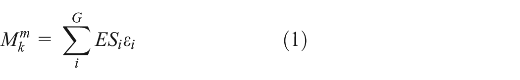
where G is the total number of girders, E is the modulus of elasticity,

where N is the number of axles,
To minimize the error function, the least-squares method is used. The partial derivative with respect to the axle weight is set to 0:
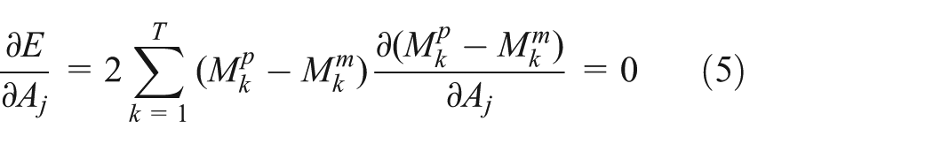
which leads to the following equation upon rearrangement and substitution

Define
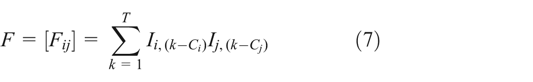

Equation (6) can then be written in a matrix form as

Thus, the axle weight and gross vehicle weight (GVW) can be calculated as


Accuracy of the Moses’ algorithm
The accuracy of the Moses’ algorithm is affected by several factors. The three most significant factors include the dynamic effect of moving vehicles, the transverse position of vehicles, and the condition of the final system equations. First of all, the dynamic effect caused by the moving vehicles reduces the accuracy of the Moses’ algorithm. This is because the Moses’ algorithm determines the axle weights through minimizing the difference between the measured and predicted bridge responses. However, the dynamic effect causes the measured response to deviate from the predicted response obtained using the static influence line and thus reduces the accuracy of the identified axle weights. From this perspective, the Moses’ algorithm usually requires that the bridge surface and approach span be in good conditions if a satisfactory accuracy is desired. Furthermore, the transverse position of the vehicle may also affect the accuracy of the Moses’ algorithm. While the transverse position of the vehicle is not considered in the original Moses’ algorithm, some researchers have found that ignoring the transverse position of the vehicle could lead to significant errors in the identified axle weights in some cases (Dempsey et al., 1999). In practice, choosing bridges with fewer lanes can limit the errors. However, even if the bridge only has one lane, which is a rare case, the transverse position of the vehicle within the lane will still have an influence on the accuracy. Also, another issue associated with bridges having more than one lane is that there might be multiple vehicles present on the bridge, which makes the identification of individual axle weight very difficult. Accordingly, some researchers proposed two-dimensional (2D) BWIM algorithms on the basis of the Moses’ algorithm to address this issue. Quilligan (2003) proposed a 2D BWIM algorithm as an extension to the Moses’ algorithm. In the 2D algorithm, the influence surface concept is used instead of the influence line. The influence surface represents the load effect caused by a unit-concentrated load at position (x, y), and the axle weights can be found by following the same minimization routine as used in the Moses’ algorithm. Theoretically, this would be an ideal solution to account for the effect of the transverse position of vehicles. However, the disadvantage of this algorithm is that it requires an accurate finite element (FE) model of the bridge, which comes at the cost of complex calculations as well as time-consuming calibrations. Alternatively, some researchers proposed other methods that modified the original Moses’ algorithm without involving the use of influence surface. Žnidaric et al. (2012) proposed a sensor strip method as an enhancement to the original Moses’ algorithm. The idea is to separate sensors into groups for each lane, and instead of summing the strains into one value at each time step, the strains are summed within each group to provide extra information on the load distribution of traffic which increases the solvability of the system equations using linear methods. Zhao et al. (2014) proposed a modified Moses’ algorithm. The proposed algorithm considered the spatial behavior of the bridge by incorporating the transverse distribution of the wheel loads on different girders to predict the bridge responses.
Another common problem encountered when implementing the Moses’ algorithm is that the derived system equations are usually ill-conditioned, especially for rough road surface (Rowley et al., 2008) and vehicles with closely spaced axles (O’Brien et al., 2009). In this case, the solution of the axle weights using the least-squares method would be sensitive to the measurement noise. This problem can be resolved by applying the Tikhonov regularization technique (Tikhonov and Arsenin, 1977) to provide bounds to the solution. An additional penalty term multiplied by a regularization parameter is added into the original minimization formulation to improve the condition of the original system. The regularization technique was reported to significantly improve the accuracy of the identified axle weights; however, as the vehicle dynamics becomes more noticeable, the convergence of the regularized solution becomes slower (O’Brien et al., 2009).
In addition, it should be mentioned that the accuracy of a WIM system is usually defined in a statistical way by the closeness of a measured value to an accepted reference value, typically within a 95% confidence interval (COST 323, 2002). The readers can refer to COST 323 (2002) for details on the target accuracy levels for different purposes.
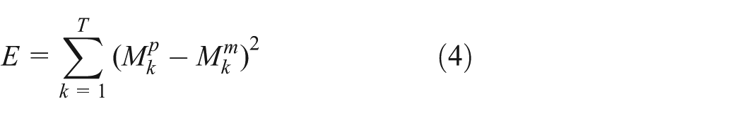
Calibration of influence lines for BWIM systems
For the Moses’ algorithm, the accuracy of the influence line is critical for the BWIM system to achieve an accurate identification. When Moses (1979) first proposed the BWIM concept, the theoretical influence line of a simply supported beam was adopted. However, the theoretical influence line could not accurately predict the real behavior of the bridge. To reduce the errors caused by the difference between the theoretical and true influence lines, Žnidaric and Baumgartner (1998) proposed an improved theoretical influence line by adjusting the support conditions and smoothing the peaks to reach better consistency with the real situation. McNulty and O’Brien (2003) proposed a point-by-point graphical method to generate the influence line. However, this method has to be executed manually, which means that its accuracy relies on the skill of the operator. O’Brien et al. (2006) presented a method to generate the influence line from direct measurements. Using the least-squares method, the error function defined in equation (4) is minimized with respect to the influence ordinate, while the axle weights of the calibration vehicle are already known, and thus, the measured response of a load effect is converted into the influence line of that effect. This method was verified by field tests and was successfully applied in a BWIM system developed by Zhao et al. (2015). However, it should be mentioned that this method generates the influence line by connecting discrete points instead of producing a smooth curve. In order to generate a continuous influence line, some researchers adopted a polynomial function to describe the influence line, and the optimal coefficients of the polynomial function are determined by minimizing the error function (Yamaguchi et al., 2009). Ieng (2015) pointed out that the method proposed by O’Brien et al. (2006) is sensitive to perturbations and revised the method on a probabilistic basis utilizing the maximum likelihood estimation principle. The revised method takes advantage of more signals in the estimation of the influence line and thus reduces the error caused by the noise in a specific signal.
Orthotropic BWIM algorithm
In the WAVE project (2001), the free-of-axle-detector (FAD) algorithm was initially developed for orthotropic deck bridges since axle detectors were not allowed on the deck surface in order to maintain the waterproofing of the deck. The idea of the FAD algorithm is to identify the vehicle speed and the axle spacing through sensors installed underneath the bridge, where the measured signal shows a sharp peak corresponding to each axle passing. For orthotropic deck bridges, the longitudinal stiffeners are usually supported by transverse cross-beams, and the supported span is usually short enough so that the strain of the longitudinal stiffeners will show a peak response corresponding to the axle passage, making them suitable for the FAD algorithm. However, it was also realized that axle detection using the FAD algorithm would be less accurate than that using traditional axle detectors. Therefore, a new identification algorithm, known as the orthotropic BWIM algorithm, was proposed (WAVE, 2001). This algorithm adopts an optimization routine using the conjugate direction methods to minimize the objective function in the form of equation (4) and thus finds the best solution of all vehicle parameters including the vehicle speed, axle spacing, and axle weights. The identified parameters from the FAD algorithm, including the vehicle speed and the axle spacing, are used as inputs into the optimization procedure, and thus, the new algorithm is less sensitive to the errors in the initially identified values of vehicle speed and axle spacing. However, if the objective function is non-convex, there will be multiple solutions for the vehicle parameters. This would require constraints being applied during the optimization procedure. In the WAVE project (2001), it was found that the vehicle speed cannot exceed 5% of its initial value for the proposed algorithm.
It should be mentioned that the Moses’ algorithm could still be applicable to the orthotropic bridges with some additional post-processing procedures. Xiao et al. (2006) instrumented the longitudinal ribs on an orthotropic box girder bridge. The response of the longitudinal ribs can be divided into a girder component, that is, the flexural stress due to the rib acting as the part of the upper flange of the box girder to support the vehicle weight and a rib component, that is, the local stress due to the rib acting as a continuous beam to support the wheel load. In the axle weight calculation, the girder component is first separated from the rib component. Then, the Moses’ algorithm is applied using the rib component to obtain the axle weights.
From the review of the above algorithms, it can be seen that the identification of axle weights through the static BWIM algorithms is essentially a mathematic optimization problem that seeks to minimize the error function which reflects the difference between the measured bridge response and the bridge response reconstructed using the vehicle parameters. In this sense, any optimization method that is capable of minimizing the error function of the form given by equation (4) can be used for the BWIM algorithms. In fact, some researchers have proposed using different optimization methods to identify the parameters of vehicles moving on the bridge. Jiang et al. (2004) and Au et al. (2004) proposed a multi-stage optimization scheme based on the genetic algorithm for the vehicle parameter identification using the acceleration responses of the bridge. Law et al. (2006) proposed an optimization method that makes use of the response sensitivity to indirectly identify the vehicle parameters. Deng and Cai (2009) applied the genetic algorithm to identify vehicle parameters in a full-scale three-dimensional (3D) vehicle-bridge system using different responses of the bridge. They found that the vehicle mass can be identified with very good accuracy, while some parameters, such as damping, are difficult to identify due to the measurement noise. Pan and Yu (2014) adopted the firefly algorithm as the optimization scheme to identify the constant moving forces. In addition to optimization methods, Kim et al. (2009) developed a BWIM algorithm based on the artificial neural networks (ANN). The algorithm is formed by two neural networks, that is, one for the GVW calculation using the signal from the weighing sensors and the other for the axle weight calculation using the signal from the FAD sensors. The training data were acquired from an adjacent pavement-based WIM station. Field tests found that the developed BWIM algorithm based on the ANN shows similar accuracy with the traditional BWIM algorithm using the influence line concept. Since the proposed ANN algorithm does not require any knowledge of the bridge behavior, it could serve as a potential tool to address the issues faced by the traditional BWIM algorithms, such as the application on long-span bridges and bridges with a rough road surface and the identification of multiple vehicles.
Influence area method
Ojio and Yamada (2002) proposed a method to calculate vehicle weights based on the principle that the area under the response curve can be expressed as the product of the GVW and the area under the influence line, that is, the influence area. This can be shown by
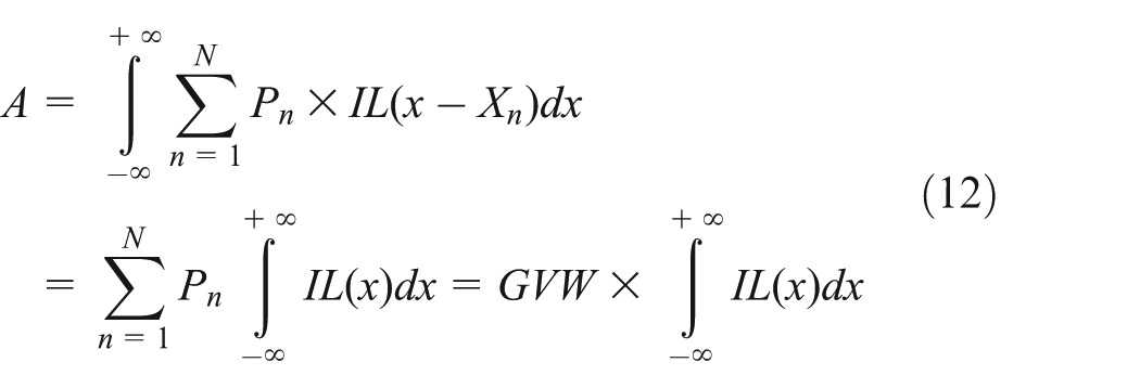
where A is the influence area, N is the number of axles of the vehicle, Pn is the axle weight of the nth axle, IL(x) is the function of the influence line, x is the position of the first axle, and Xn is the distance from the first axle to the nth axle. The area under the response curve can be obtained by numerically integrating the response of the bridge. Thus, with a calibration vehicle of a known weight, the weight of another vehicle with unknown weight can be obtained by

where GVW is the gross vehicle weight of the unknown vehicle, A is the area under the response curve for the vehicle with the unknown weight, Ac is the area under the response curve for the calibration truck, and GVWc is the GVW of the calibration truck. While the implementation of this algorithm is easy and does not require axle detections, one obvious disadvantage is that identifying the weight of individual axles becomes very difficult. Thus, this method is more suitable for cases where the axle weights of the vehicle are not of interest (Cardini and DeWolf, 2009).
Reaction force method
Ojio and Yamada (2005) proposed a method where the measured reaction force at the support is used to calculate the axle weights. This method utilizes the influence line of the reaction force of a simply supported bridge. An important feature of such an influence line is that a sharp edge appears at the beginning of the influence line, since the maximum value of the reaction influence line occurs as the unit load first presents on the bridge. The edge can be assumed to be solely contributed by the axle load, since it is generated in a very short time. Thus, the axle weights can be calculated from the height of the edge.
The reaction force method is simple and easy to implement. Furthermore, an edge will appear in the signal, as each axle of the vehicle enters the bridge, and thus, it can also be used for the purpose of axle detection. However, this method has not been extensively applied in practice due to the following drawbacks: (1) the reaction force method uses only the peak strain of the response instead of the entire time history of the response, and thus, the dynamic effect of the axle forces is not accounted for, which, in turn, causes errors in the identified axle weights; (2) the reaction forces are difficult to measure in practice; and (3) the method is only applicable to right-angled bridges.
Moving Force Identification
The MFI method seeks to obtain the complete time history of the vehicle axle forces when a vehicle passes the bridge. The MFI method has the potential to be very accurate in the identification of static axle weights, since the complete history of the time-varying forces will allow the dynamic effects of the vehicle to be identified and removed when calculating the static axle weights. The MFI theory has been developed since the 1990s when several classic MFI methods were proposed including the interpretive method (IM), the time domain method (TDM), and the frequency–time domain method (FTDM).
Interpretive Methods
O’Connor and Chan (1988) proposed an IM in which the beam is modeled as an assembly of lumped masses interconnected by massless elastic beam elements. The identification process is treated as an inverse problem to the predictive analysis for the beam in which the dynamic responses of the beam are derived as


where
Chan et al. (1999) proposed another IM which uses the Euler’s beam theory instead of the beam-element model. The equation of motion of the Euler–Bernoulli beam can be written as

where
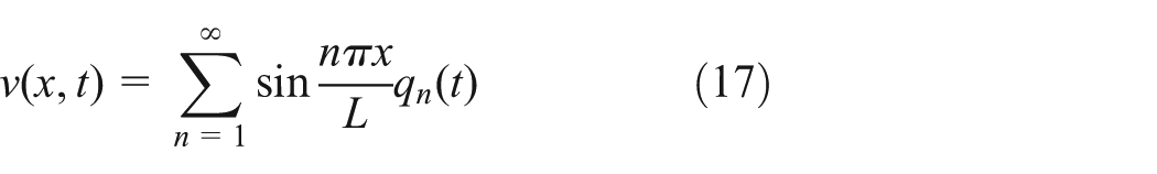
where

where
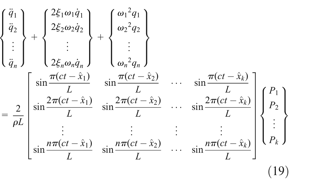
where
To obtain the time history of the axle forces, the measured response is first transferred to the modal displacement. Then, the numerical differentiation method is used to obtain the modal velocity and acceleration from the modal displacement. Therefore, equation (19) again becomes an over-determined set of linear equations where the axle load
Time Domain Method
Law et al. (1997) developed a system identification method based on the modal superposition principle. In their method, the dynamic deflection can be obtained by solving equation (16) in the time domain using the convolution integral
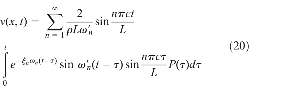
where
Frequency-time Domain Method
Law and Chan (1999) proposed the FTDM, where equation (16) is solved in the frequency domain to identify the axle forces. The Fourier transformation of the deflection
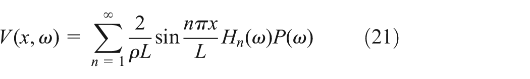
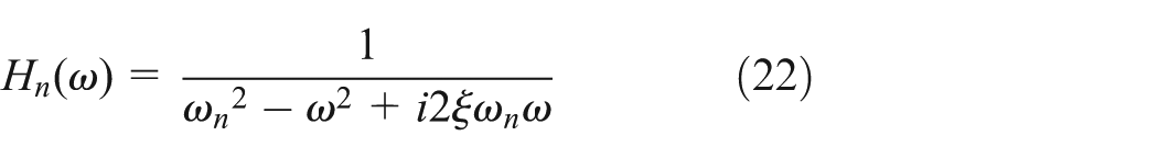
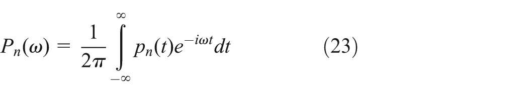
where
Similarly, the real and imaginary parts of
It can be seen that for the above MFI methods, the problem eventually becomes solving the linear algebraic equation of the form

where A is an m-by-n matrix. In the case of MFI problems, m is larger than n and the over-determined set of system equations can be solved using the least-squares method leading to

where A+ denotes the pseudo-inverse (PI) of the matrix A, and x is called the PI solution. In order to be able to obtain this PI solution, A needs to have a full rank. However, it was found that sometimes there exists linear dependency in A, which would increase the error of the PI solution (O’Connor and Chan, 1988). To overcome this problem, the singular value decomposition (SVD) technique can be used to calculate A+. In fact, it has been shown by some studies that using the SVD can significantly improve the accuracy of the identified force history, especially for the FTDM (Yu and Chan, 2002, 2003, 2007). However, it was still found that the identified results are sensitive to noise and exhibit large fluctuations, since the nature of the inverse problem is ill-conditioned. In this case, regularization is necessary to provide bounds to the solution. Many researchers adopted the Tikhonov regularization method and found that the regularization is very effective in reducing the effect of noise on the identification accuracy (Deng and Cai, 2010; Law et al., 2004; Law and Fang, 2001; Law and Zhu, 2000; Zhu and Law, 2000, 2002a). Nevertheless, this method requires finding the optimal regularization parameter using methods such as cross-validation (Golub et al., 1979) and the L-curve method (Hansen, 1992), which is usually time-consuming. To resolve this issue, Pinkaew (2006) proposed a regularization method using the updated static component (USC) technique and found that the identification accuracy using the USC technique is not sensitive to the regularization parameter, and that the identification using the USC technique actually provides a better accuracy than the conventional regularization method (Asnachinda et al., 2008; Pinkaew, 2006; Pinkaew and Asnachinda, 2007).
Following the development of the classic MFI theories, some comparative studies have been conducted to investigate the effectiveness of the four methods under different conditions and the sensitivity of each method to the errors in the vehicle-bridge parameters and the measurement parameters (Chan et al., 2000b, 2001a, 2001b; Yu and Chan, 2007; Zhu and Law, 2002b). Furthermore, much effort has also been made to improve the accuracy and to extend the applicability of existing MFI algorithms. Zhu and Law (1999) extended the IMII to a continuous bridge which is modeled as a multi-span Timoshenko beam. Chan et al. (2000a) and Chan and Yung (2000) applied the TDM and the IMI in the MFI on pre-stressed concrete bridges considering the pre-stressing effect in the beam model. Zhu and Law (2000) extended the TDM to a bridge deck that is modeled as an orthotropic plate and introduced the Tikhonov regularization to provide bounds to the identified force. Zhu and Law (2001) used the exact solution of the mode shapes considering the rigid support condition for the IMII, which eliminates the modeling errors from the assumed mode shapes. Also, they adopted the generalized orthogonal function to obtain the derivatives of the bridge modal response so as to reduce the errors due to the measurement noise. Zhu and Law (2003) revised the way that the system matrices are calculated in the TDM, which improved the computational efficiency of the method. Zhu and Law (2006) applied the TDM on a multi-span bridge deck that is modeled as an Euler–Bernoulli beam with elastic restraints at the supports. Chan and Ashebo (2006) proposed identifying moving forces on continuous bridges using the TDM by considering the response of only one of the spans. Asnachinda et al. (2008) presented a method to identify multiple vehicles on a continuous bridge based on the FE method, where the bridge is modeled as a continuous Euler–Bernoulli beam. Dowling et al. (2012) adopted the cross-entropy optimization method to infer the material properties required to form the mass and stiffness matrices and thus solved the issue of FE model calibration for the MFI algorithm.
Meanwhile, some novel MFI algorithms have been proposed. Law and Fang (2001) developed a new method for the MFI based on the state-space formulation and dynamic programming, which inherently provides bounds to the ill-conditioned force. Law et al. (2004) presented an MFI method based on the FE method and the improved system condensation technique. The error caused by the modal truncation is thus eliminated by expressing the measured displacements as shape functions. Law et al. (2008) introduced a new MFI method based on the wavelet decomposition and FE method. This method requires no assumption on the initial condition of the system. Deng and Cai (2010, 2011) proposed a new identification method based on the superposition principle and influence surface and adopted a 3D FE model for the bridge used in their studies. Wu and Law (2010) presented a stochastic identification algorithm that can deal with complex random excitation forces with large uncertainties and system parameters with small uncertainties. The algorithm is formed based on the established statistical relationship between the random excitation forces and the structural responses which are assumed to be Gaussian and are represented by the Karhunen–Loéve expansion.
Despite the fact that the MFI methods have the potential to be very accurate and ideal for direct enforcement, there are still many challenges to implement the MFI algorithms in the modern commercial BWIM systems. First, the MFI is computationally expensive and thus, it may be difficult to achieve the real-time identification of axle weights. Furthermore, most of the previous studies on the MFI are still based on overly simplified bridge models such as simple beams and plates. However, in practice, 3D bridge models must be adopted in order to accurately reflect the behavior of the bridge. The Moses’ algorithm, on the other hand, is simple to implement. As long as certain requirements are met, the accuracy of the Moses’ algorithm can satisfy the requirements for direct enforcement, which makes the Moses’ algorithm the optimal choice for modern commercial BWIM systems. Other static algorithms have distinctive limitations and are, thus, not suitable for direct enforcement, but they can provide alternatives when the Moses’ algorithm is not suitable.
Instrumentation of BWIM systems
An on-site BWIM system usually consists of a data acquisition system, a communication system, a power supply system, and sensors. For example, Figure 1 shows the components of the SiWIM system, a commercially available BWIM system that was originally developed within the framework of the WAVE project (2001) and has been continuously improved and updated over the years. The data collected from the on-site system are processed with software using BWIM algorithms. The results are then presented in a graphical user interface (GUI) that is designed for users to visualize the real-time monitoring data. The following sections will introduce the typical instrumentation of BWIM systems including the types of sensors used in a BWIM system and their installation locations.
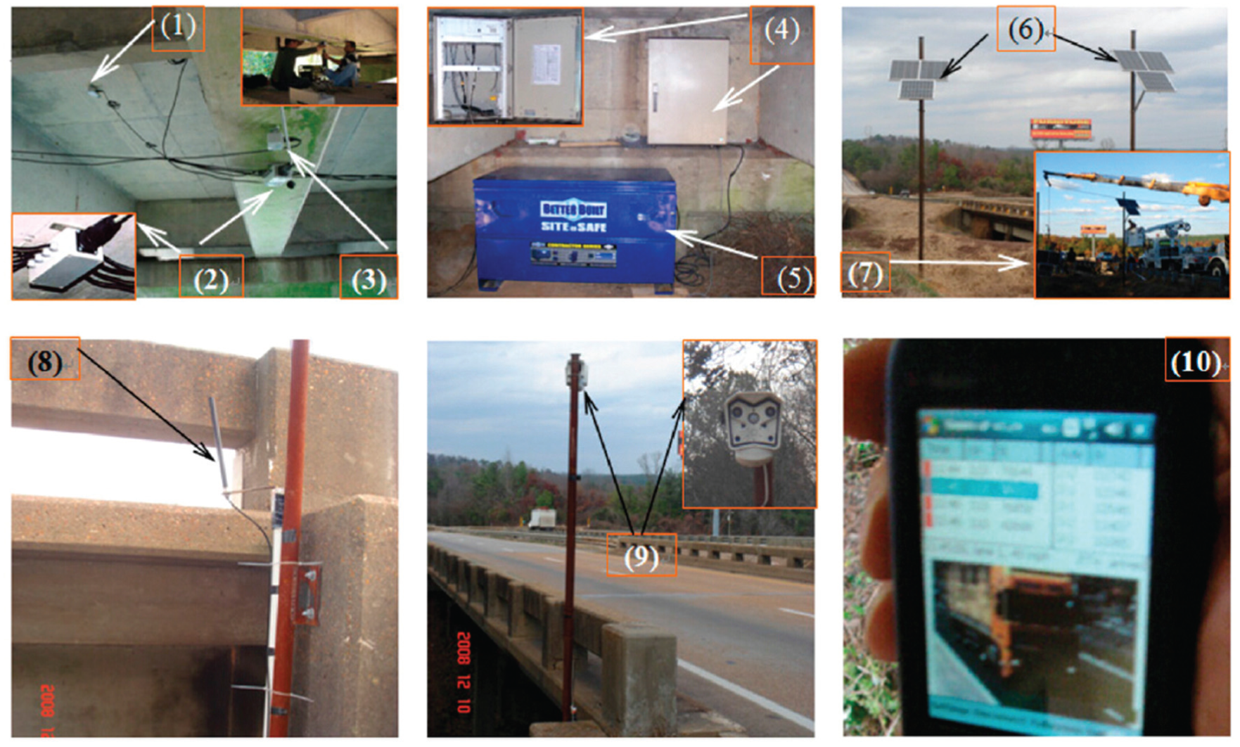
Components of an SiWIM system: (1) FAD sensors, (2) spider, (3) weighing sensors, (4) cabinet and panel, (5) batteries, (6) solar panels, (7) solar panel installation, (8) antenna, (9) camera, (10) PDA.
Strain measurement
In a modern BWIM system, the sensors can be divided into two main categories, that is, the weighing sensors and the axle-detecting sensors. Weighing sensors usually measure the global bending strain of the bridge due to the vehicle loading which serves as the main input for the calculation of axle weights, that is, the measured strain in a certain girder
Foil strain gauges
Foil strain gauges have been commonly used for strain measurements. When the measured material is strained, the foil will deform and cause the electrical resistance to change. This change is calibrated to reflect the equivalent change in strain. Foil strain gauges can be attached to the surface of the structural components. They are cheap and have acceptable accuracy, which makes them suitable for experimental tests and short-term measurements. However, they are not suitable for long-term field measurements as in the case of BWIM systems due to their poor durability and susceptibility to electromagnetic interferences and environmental changes.
Vibrating wire strain gauges
Vibrating wire strain gauges can either be embedded in concrete or mounted on the surface of structural components. It works based on the principle that the change in strain will cause a change of the tension in the wire, which leads to the variation in the resonant frequency of the wire. Vibrating wire strain gauges have good durability, and their installation requires little surface preparation. However, the vibrating wire strain gauge has a low scanning rate, which makes it difficult to record the dynamic response of the bridge when the vehicle travels at a high speed.
Fiber optic sensors
Fiber optic sensors, especially FBG sensors, have become increasingly popular in the field of structural health monitoring (SHM). FBG sensors use the relationship between the change of the wavelength in the reflected spectrum and the strain induced by forces or temperature changes to measure the strain. FBG sensors have the following advantages when compared to conventional strain gauges: (1) FBG sensors are immune to electromagnetic interferences, which eliminates the noise from external sources to a certain degree; (2) FBG sensors have good durability, which makes them suitable for long-term measurements; and (3) FBG sensors have small sizes and can be multiplexed, which allows easy installation of multiple sensors on large structures. These advantages have made FBG sensors an excellent candidate for BWIM applications. Recent studies have also found that using FBG-based sensors improved the accuracy of the BWIM system overall (Lydon et al., 2014, 2015).
Axle detection
In a modern BWIM system, axle-detecting sensors are used to identify the presence of vehicle axles from which the speed and axle spacing of the vehicle can be calculated. Axle detection is an indispensable part of the BWIM system, since the identified vehicle speed and axle spacing of the vehicle will directly affect the results of the axle weight calculation. The traditional instruments for axle detection include tape switches and pneumatic tubes. Moses (1979) pointed out that tape switches are easier to be incorporated into the system, while the pneumatic tubes require a pressure-sensing device to produce the signal of axle passage. The identification of vehicle speed and axle spacing using traditional axle detectors is actually quite simple. Usually, two parallel axle detectors are placed on the road surface, where the spacing between the two detectors is measured as an input into the system. In some cases, where the transverse location of the vehicle needs to be determined, a third detector is placed diagonally with a known angle corresponding to the other two detectors. Nevertheless, the installation of axle detectors on the pavement usually requires lane closure, and the poor durability of sensors also diminishes the advantage of the BWIM systems over the pavement-based WIM systems.
To overcome the problems of the traditional axle detection, the FAD algorithm was first proposed in the WAVE project (2001). The basic idea of the FAD algorithm is to use FAD sensors to replace traditional axle detectors on the road surface. The FAD sensors measure the local strain responses, and thus, they pick up a sharp peak upon each axle passage above the sensor location. Typically, two FAD sensors are installed at different longitudinal locations on each lane with a known distance. Figure 2 shows some typical signals of the FAD sensors, which were recorded when a five-axle truck passed through the bridge (Zhao et al., 2014). It can be seen that each FAD sensor picked up five peaks corresponding to the five axles. However, it should be mentioned that clear peaks in the strain signal might not occur if the wheel load is directly applied over the beam (Lydon et al., 2015). In practice, a correlation function is usually used to calculate the vehicle speed. The correlation function is defined as
where f(t) and g(t) are the signals of the FAD sensors at two longitudinal locations, respectively. To calculate the vehicle speed, the time taken by the vehicle to pass the known distance between the two sensors is needed. From equation (27), it can be seen that the correlation function will reach the maximum value when f(t) and
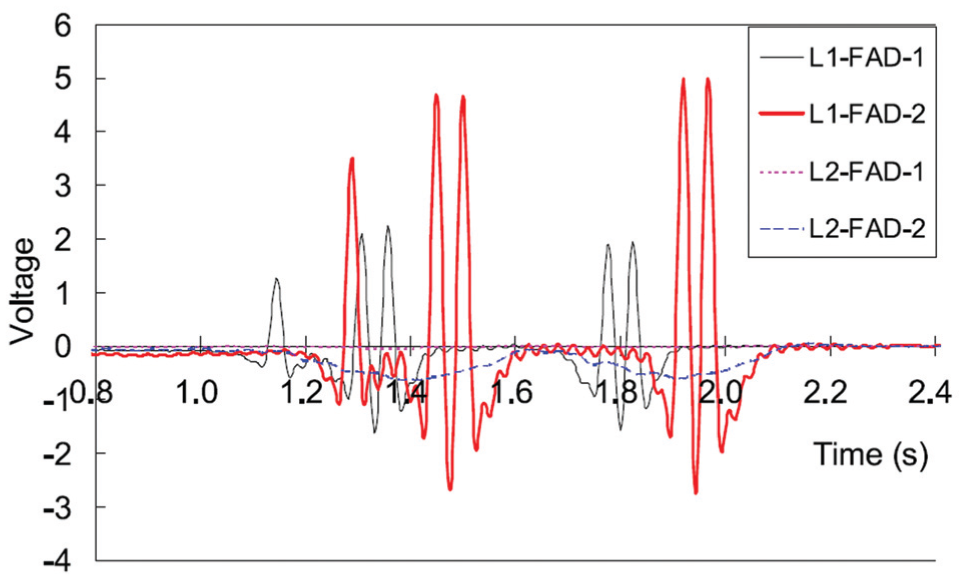
Typical FAD signals of a five-axle truck crossing.
Although the FAD algorithm resolves the durability problem of the traditional axle detectors, it still requires additional sensors, that is, the FAD sensors, only for the purpose of axle detection. Furthermore, the FAD algorithm imposes certain restrictions upon the span length and superstructure thickness of the selected bridge. Namely, the FAD algorithm is not applicable to all types of bridges. As a general rule of thumb, the bridges suitable for the FAD algorithm should have the following: (1) a short span or relatively longer span but with transverse supports, that is, secondary members such as transverse cross-beams or stiffeners, to divide the bridge into sub-spans, because longer spans will have joint contributions of several axles that make it difficult to distinguish individual axles; (2) a thin superstructure, because a thick superstructure will “smear” the peaks induced by the vehicle axles; and (3) a smooth road surface and approach span, since a rough surface condition will cause significant dynamic effects which impose additional peaks into the signal (Kalin et al., 2006; WAVE, 2001). The types of bridges that have already been identified as suitable for the FAD algorithm include orthotropic deck bridges, short integral bridges with thin slabs (usually 6–12-m long with the slab thickness between 40 and 60 cm), and beam-slab bridges with secondary members (WAVE, 2001).
Recently, the concept of a nothing-on-road (NOR) BWIM system was proposed. The goal of the NOR BWIM system is to free the use of axle detectors on the road surface. While the FAD algorithm is one application of the NOR BWIM, a more effective way is to directly employ the global strain signal obtained from the weighing sensors to identify the vehicle speed and axle spacing. This will be a very attractive feature for future commercial BWIM systems, since it reduces the number of sensors required and thus the cost of the system, making the installation even easier. Besides, it does not impose any restriction on the selection of bridges, which helps extend the application of BWIM technologies. However, direct identification from the global strain signal is very difficult, since it usually does not have a sharp peak upon each axle passage. Nevertheless, it has been shown by some researchers that the identification can be achieved through proper signal-processing techniques such as a wavelet-based analysis, which are suitable to treat non-stationary signals. Dunne et al. (2005) first proposed using wavelet transformation to identify closely spaced axles from the FAD signals. Chatterjee et al. (2006) conducted field testing on a culvert and adopted the wavelet transformation to analyze the strain signal obtained from vehicle crossing. The results show that the wavelet techniques can help identify closely spaced axles within a tandem or tridem group which could not be directly identified from the FAD signal and reveal the potential of using the wavelet techniques to identify vehicle axles from the strain signal of weighing sensors. Yu et al. (2015) proposed a vehicle axle identification method based on the wavelet transformation of the global signal. The numerical results showed that this method could provide accurate identification of vehicle axles using only the weighing sensors.
In addition, some other methods for axle detections have also been reported. Some researchers found that crack openings on the bottom of the concrete slabs are sensitive to axle loads, and thus, they measured the changes in the widths of existing cracks to detect the vehicle axles (Lechner et al., 2010; Matui and El-Hakim, 1989). However, this method cannot be generalized, since it is only applicable to bridges with crack openings. Wall et al. (2009) adopted an approach where the change of slope induced by the axle passage is used for the axle identification. In an ideal setting, the passage of each axle will have a corresponding impulse in the second derivative of the strain signal. However, in practice, this approach requires the strain signal to have evident slope discontinuities; in other words, the strain signal must show a certain level of sensitivity to the vehicle axles. Also, as these slope discontinuities are only subtle changes, this approach may no longer be feasible once the measurement noise is introduced in practice. O’Brien et al. (2012) proposed a novel axle detection strategy using shear strain sensors based on the assumption that each axle passage will induce a sudden change of the shear strain. Preliminary FE analyses were carried out on a beam-slab bridge, and the interface of the web and the flange was recommended for the sensor locations. Further work was planned in order to assess the feasibility of this novel axle detection method. In addition, with the recent advances in the image-processing technologies, the identification of the vehicle axle configuration has been made possible through proper image analysis algorithms, and thus, a vision-based system utilizing a roadside camera was proposed by some researchers as a potential tool for the axle detection (Caprani et al., 2013; Ojio et al., 2016).
Installation location of sensors
The sensor installation locations should account for several factors including the function of sensors, types of bridges, strain levels, sensitivity-to-strain variations, and so on. In this section, the sensor installation locations will be discussed with respect to the two most important factors, that is, the function of sensors and types of bridges chosen for installation. In addition, a case study with specific sensor layouts on a typical beam-slab bridge is also presented.
Function of sensors
Weighing sensors measure the global bending strain caused by vehicle loads, and thus, they are usually installed at locations of the most pronounced responses, for example, the mid-span of the bridge. Nevertheless, it is interesting to note that other installation locations have also been reported for weighing sensors. For example, in the reaction force method proposed by Ojio and Yamada (2005), the weighing sensors were attached to the end vertical stiffeners above the supports of a steel plate girder bridge to measure the strain for the bearing. For complex bridge structures, the locations of weighing sensors can be determined by a preliminary FE analysis. As for axle-detecting sensors, both the traditional axle detection and the FAD algorithm require two parallel lines of sensors to be installed at a known distance. However, the differences are the following: (1) the traditional axle-detecting sensors are installed on the road surface, while the FAD sensors are installed underneath the bridge; (2) the traditional axle-detecting sensors can be installed at almost any location on the bridge; however, the selection of the installation locations for the FAD sensors depends on the shape of the influence line, since the influence line at the location of installation needs to present a sharp peak in order for the axle identification.
Types of bridges
The sensitivity of strain responses to axle loads differs between different bridge types and different measurement locations on a certain bridge; thus, the specific plan of sensor layouts for each bridge should be determined on a case-by-case basis. Nevertheless, based on the existing BWIM practices, the general schemes of sensor layouts for some typical bridges are summarized and shown in Table 1. It should be mentioned that the reason for requiring only one line of axle-detecting sensors in orthotropic deck bridges is that the installed weighing sensors can also pick up sharp peaks corresponding to the axle passage, namely, the weighing sensors in this case also serve the purpose of axle detection.
General layout schemes of BWIM sensors for typical types of bridges.
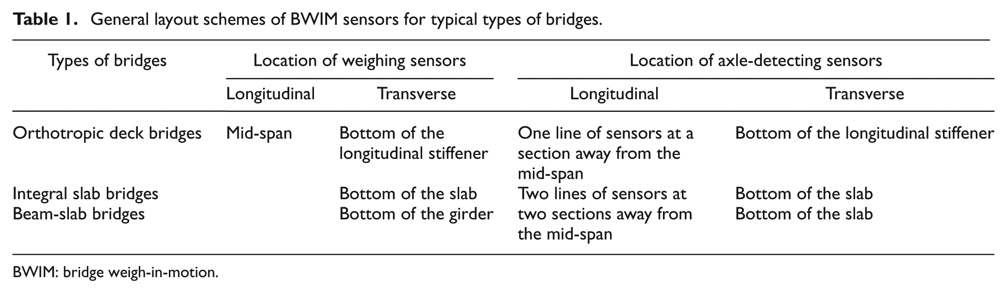
BWIM: bridge weigh-in-motion.
In addition, Brown (2011) studied the influence of different installation schemes of FAD sensors on the accuracy of axle detections, including the longitudinal and transverse locations, and installation angles. Based on the signals obtained from a T-beam-reinforced concrete bridge, it was concluded that FAD sensors should be orientated longitudinally and installed close to the beginning or the end of the bridge span, ideally directly below the wheel path, in order to obtain a clear signal with sharp peaks. The reason for choosing the beginning or the end of the bridge span is that the bridge is stiffer at these locations, and thus, more definite peaks can be produced. The dynamic effects at these stiffer locations are also less pronounced, which leads to a cleaner signal. Furthermore, the study also shows that compared to longitudinally orientated sensors, transversely orientated sensors provide poor signals for axle detection. Besides, it was also found that weighing sensors do not have to be installed exactly at the mid-span, since any location near the mid-span can provide an adequate strain level for weighing purposes.
Case study
In order to give a better illustration on the sensor installation of the BWIM system, a case study is presented here. The case study is chosen from a recent BWIM practice conducted by Zhao et al. (2014) in Alabama. The instrumented bridge is a three-span simply supported concrete multi-girder bridge. The three spans have an equal length of 12.8 m, and the first span was chosen for the installation of the BWIM system. The reasons for selecting this bridge are as follows: (1) the bridge has a short span and thin superstructure, suggesting that it is suitable for the implementation of the FAD algorithm; (2) the short span has higher natural frequencies to avoid matching the natural and pseudo frequencies of the vehicle and thus reduces the dynamic effect of the moving vehicles; and (3) the bridge has a smooth approach and a good surface condition, which again helps minimize the dynamic effect.
For the sensor installations, a total of four weighing sensors were installed in a parallel manner underneath the girders (one for each girder), and a total of four FAD sensors were mounted beneath the concrete slab (two for each lane). The specific sensor layouts are presented in Figure 3. It should be noted that the sensors are not installed exactly at the mid-span because of the diaphragm.
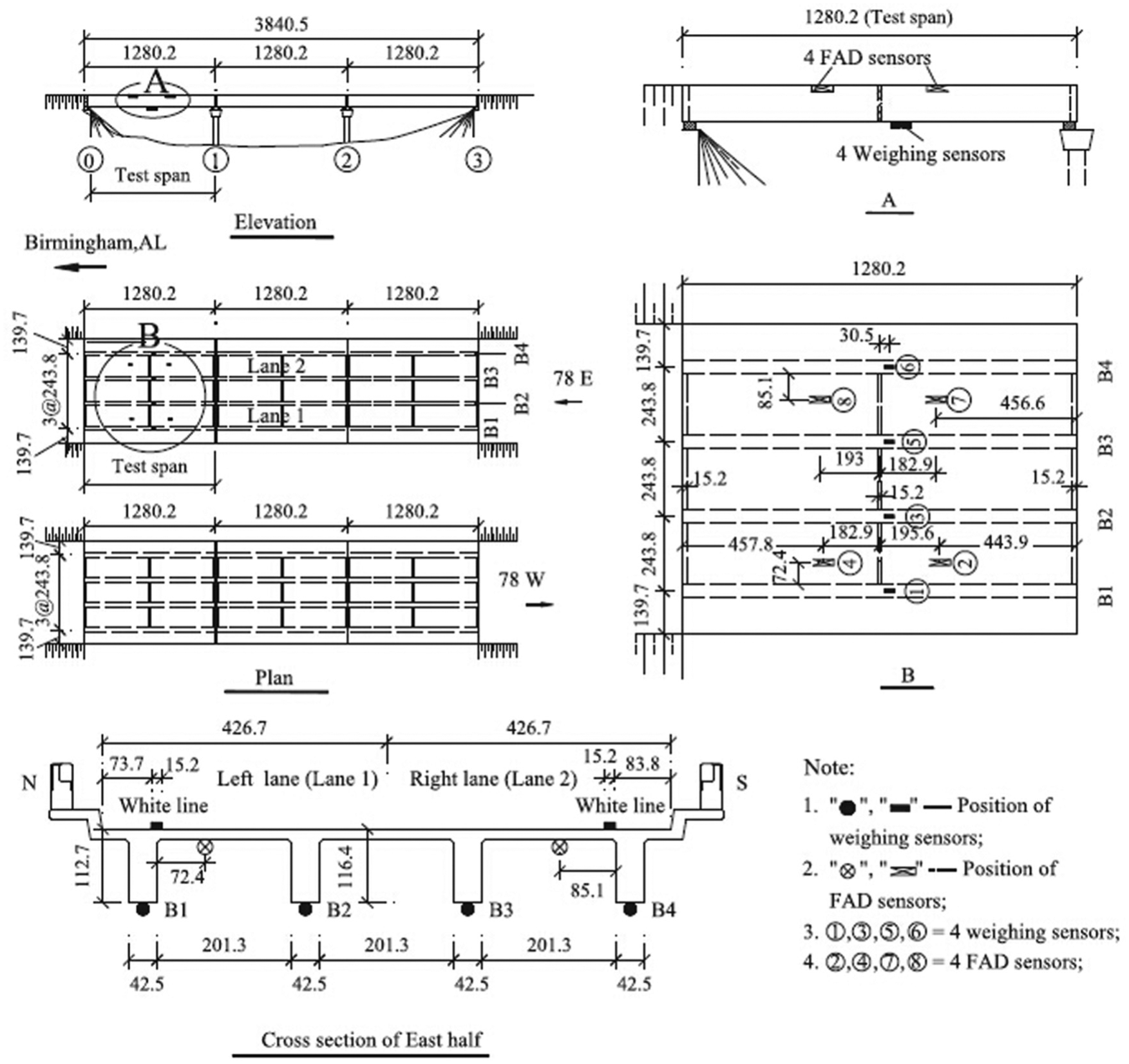
Sensor layouts of a typical BWIM system (cm).
Data acquisition and storage
In a BWIM system, the collection of raw data from the sensors is achieved through an on-site data acquisition system. The sensors communicate with the data acquisition system by wired or wireless connections. The core of a data acquisition system is a well-designed algorithm of data sampling and recording. Based on the Nyquist–Shannon sampling theorem, it is suggested that the sampling frequency for the data collection be at least twice the maximum vibration frequency of interest so as to prevent the folding and aliasing problems when digitizing the data (Paultre et al., 1995). In practice, the sampling frequency may be higher and an anti-aliasing filter may be necessary as well. However, the sampling frequency should not be too high as this will result in a huge volume of data being stored. Nevertheless, in terms of long-term monitoring, the amount of produced data will still be enormous. This problem can be resolved by establishing an event-triggering mechanism, that is, the strain data will only be recorded and stored when a critical event, which is defined as a truck with a certain weight that is larger than the minimum weight of interest passes through the bridge. This can be done by setting a lower limit for the sensor, and the value of the lower limit is determined by the maximum response caused by the load corresponding to the minimum truck weight. In this case, only those critical events under which the bridge responses equal or exceed the lower limit will be recorded, and thus, the amount of stored data will be significantly reduced.
Conclusion and remarks
This article presents a comprehensive review on the state-of-the-art BWIM technologies from two important perspectives, that is, the BWIM algorithms and instrumentation of BWIM systems. On the basis of recent developments achieved in the field, the following conclusions can be drawn and remarks can be made:
The BWIM technique has significant advantages over the pavement-based WIM technique. BWIM systems are more durable, and their installations are also easier and safer. Moreover, BWIM systems are potentially more accurate than pavement-based WIM systems.
The static BWIM algorithms include the Moses’ algorithm, the influence area method, the reaction force method, and the orthotropic BWIM algorithm. Although the accuracy of the Moses’ algorithm depends on several factors, it is straightforward and relatively simple to implement. The influence area method can be used to estimate the GVW; however, it is difficult to identify the weight of individual axles. The reaction force method is simple to implement; however, some drawbacks have limited its extensive applications. The orthotropic BWIM algorithm employs a different optimization scheme and can serve as an alternative to the Moses’ algorithm in some cases.
The MFI methods, that is, the dynamic BWIM algorithms, have the potential to be very accurate. However, they also have distinctive drawbacks when compared to the static BWIM algorithms, including expensive computation and requiring detailed FE model of the bridge. Besides, most of the current MFI theories are still based on simple bridge models. These disadvantages have made it difficult to implement the MFI algorithms in modern commercial BWIM systems.
In a modern BWIM system, weighing sensors are used to measure the global strain responses of the bridge. Of all the candidates for weighing sensors, FBG sensors are considered the most suitable for the BWIM application, since FBG sensors have many advantages over the traditional strain gauges such as the ease of installation, capability of multiplexing, good durability, and electromagnetic immunity.
The traditional axle detectors have been gradually replaced by the FAD sensors in the modern BWIM systems. The FAD algorithm utilizes the sharp peaks in the local strain responses measured by FAD sensors to identify the axle presence. Nevertheless, a more effective approach to achieve the NOR BWIM is to identify vehicle axles from the signals of weighing sensors through the use of well-chosen signal-processing techniques. The implementation of such an axle identification scheme would further simplify the installation and reduce the cost of BWIM systems.
Through the review of the recent developments of BWIM technologies, the following issues are identified, and corresponding suggestions for the future research are tentatively proposed:
The application of BWIM techniques on long bridges has rarely been studied. This is because of the following: (1) the possibility of multiple-vehicle presence, which is difficult to identify, increases in long bridges; (2) longer bridges have lower natural frequencies that are more likely to match the vehicle frequencies and thus increase the dynamic effect; (3) the speed of the vehicle is more likely to change during the crossing on long bridges; and (4) it is easier to identify closely spaced axles in shorter bridges (WAVE, 2001). To overcome these difficulties and achieve the implementation of BWIM systems on long bridges, future research may refer to unconventional methods such as a neural network as possible alternatives to the traditional BWIM algorithms whose accuracies are susceptible to the occurrence of multiple-vehicle presence and significant dynamic effects caused by either a rough road surface or the frequency matching between the vehicle and bridge.
Even though the MFI methods have the potential to be very accurate, it is still not fully ready to be implemented in the modern commercial BWIM systems. This is because of the following: (1) the MFI algorithms are computationally demanding, which makes it difficult to achieve the real-time identification of vehicle parameters; (2) the MFI algorithms require an accurate FE model of the bridge that is usually difficult to obtain; and (3) most of the proposed MFI algorithms are still based on simple models that may not be able to accurately represent the real behavior of bridges. Nevertheless, the MFI is still considered to be a very promising algorithm for future commercial BWIM systems. Thus, future research should focus on employing optimization and condensation methods to reduce the calculation efforts and extending the current MFI theories to 3D bridge models.
Although the current practice of the FAD algorithm has been proven to be successful on certain types of bridges, it still requires additional FAD sensors to identify the vehicle axles, and the algorithm also imposes restrictions on the selection of bridges, which limit its applications. Naturally, a more advanced method of achieving the NOR BWIM is to identify all vehicle parameters from the weighing sensors. This will be considered as a very attractive feature in the future development of commercial BWIM systems. Nevertheless, current studies on this topic are still limited and are based on simple bridge models. More research should be conducted to explore the effectiveness of identifying vehicle speed and axle spacing from the strain signals of weighing sensors and to extend the identification algorithm to more complex bridge structures.
The information extracted from BWIM systems can also be used for the purpose of SHM or vice versa. There have been some recent investigations on the use of BWIM systems for damage detection (Cantero et al., 2015; Cantero and González, 2015; Carey et al., 2013; Zhu and Law, 2015) and determination of dynamic amplification factors (O’Brien et al., 2013; Zhao and Uddin, 2014). In the future, more research can be focused on incorporating BWIM technologies into the SHM systems to further extend their applications and reduce the cost of SHM systems.
Footnotes
Declaration of Conflicting Interests
The author(s) declared no potential conflicts of interest with respect to the research, authorship, and/or publication of this article.
Funding
The author(s) disclosed receipt of the following financial support for the research, authorship, and/or publication of this article: The study was financially supported by the key basic research project (973 projects) of P.R. China, under contract no. 2015CB057701 and by the Louisiana Transportation and Research Center (no. 13-2ST). The contents presented reflect only the views of the authors.