
Abstract
Adding vertical ribs is recognized as a useful practice for reducing wind effects on cooling towers. However, ribs are rarely used on cooling towers in China since Chinese Codes are insufficient to support the design of rough-walled cooling towers, and an “understanding” hampers the use of ribs, which thinks that increased surface roughness has limited effects on the maximum internal forces that control the structural design. To this end, wind tunnel model tests in both uniform flow field with negligible free-stream turbulence and atmospheric boundary layer (ABL) turbulent flow field are carried out in this article to meticulously study and quantify the surface roughness effects on both static and dynamic wind loads for the purpose of improving Chinese Codes first. Subsequently, a further step is taken to obtain wind effects on a full-scale large cooling tower at a high Re, which are employed to validate the results obtained in the wind tunnel. Finally, the veracity of the model test results is discussed by investigating the Reynolds number (Re) effects on them. It has been proved that the model test results for atmospheric boundary layer flow field are all obtained in the range of Re-independence and the conclusions drawn from model tests and full-scale measurements basically agree, so most model test results presented in this article can be directly applied to the full-scale condition without corrections.
Introduction
Large cooling towers may experience strong wind events in their service durations, which are basically a classic scenario of flow past a circular cylinder at a high Reynolds number (Re). Researches concerning this topic are of both practical and theoretical significance. Based on endeavors made during the past a few decades, it is concluded that there are three important parameters influencing the flow states in this event: the Re, the turbulence intensity of the oncoming flow, and the surface roughness of the cylinder (Niemann and Hölscher, 1990). Among these parameters, only the surface roughness of the cylinder can be adjusted for reduced wind effects on cooling towers in practice. It has been found that increased surface roughness on cooling towers can lead to equalized mean wind pressure distributions and reduced stresses in the shells (see, e.g. Farell et al., 1976). In this regard, vertical ribs have been arranged on many cooling towers’ external surfaces to increase the surface roughness in many countries.
However, vertical ribs are seldom used on large cooling towers in China to reduce wind effects. This is mainly due to the deficiency of the Chinese Codes (GB/T 50102-2003, 2003; DL/T 5339-2006, 2006) in providing technical supports for such design. Chinese Codes fail to give mean wind pressure distributions for rough-walled towers. The German Code VGB-R 610Ue (2005), on the other hand, sets a good example providing six standardized pressure distribution curves for different surface roughness. However, VGB-R 610Ue includes some simplifications and conservatism, which need to be figured out before it can be used as the reference for improving Chinese Codes. At present, a detailed study on the influence of surface roughness on the mean wind pressure distribution is required. Besides, the dynamic wind effects on cooling towers are also important topics, such as the fluctuating wind pressure distribution and the Strouhal number (St) of vortex shedding. The former is an important contribution to the extreme wind loads, and the latter directly relates to the frequency of vortex shedding which should be examined to prevent vortex-induced vibration. Since little is known about the influence of increased surface roughness on the dynamic wind effects, related research can also be rewarding.
Another thing that hampers the use of the vertical ribs on cooling towers in China is an “understanding” that adding vertical ribs causes difficulty in construction and has limited potentials for saving materials. Specifically, it is thought that the controlling internal forces for adding reinforcements in structural design are generally the tensile stress and the bending stress at the stagnation point. With the increase in surface roughness, the changes in mean wind pressure coefficients are mainly at the side regions, which have little effects on the internal forces in the shell near the stagnation point. This “understanding” needs to be validated first. Even if supportive evidences have been found for it, it is still not a very deliberate consideration because it only pays attention to the local structural behaviors and disregards the influence of surface roughness on the overall structural stability. In fact, the overall structural stability is engineers’ major concern in designing a cooling tower against extreme events. Due to the limited article length, this topic is not available for this study, but will be investigated in the future.
In the article, pressure measurements on a 1:200 scaled cooling tower rigid model are conducted in a wind tunnel. Eight types of surface roughness are simulated on the model for meticulous study of the influence of surface roughness on both static and dynamic wind effects. Besides, full-scale measurements on an actual 167-m high smooth-walled cooling tower are carried out at a high Re. The purpose of full-scale measurements is to examine the effectiveness of wind tunnel model tests, and some consistent conclusions drawn from both tests are of practical significance.
Wind tunnel model test
Overview of test
The wind tunnel test is carried out in TJ-3 atmospheric boundary layer (ABL) wind tunnel at Tongji University, Shanghai. It is a closed circuit rectangular cross-section wind tunnel, wherein the size of the test zone is 15 m in width, 2 m in height, and 14 m in length. The test wind speed can be continuously controlled in a range from 1 to 17.6 m/s. In uniform flow field, the non-uniformity of wind speed in test zone is less than 1%, the turbulence is less than 0.5%, and the average flow deviation angle is less than 0.5°. Besides the uniform flow field, the ABL turbulent flow field of Type B according to Chinese Codes is also simulated for the test, as shown in Figure 1.
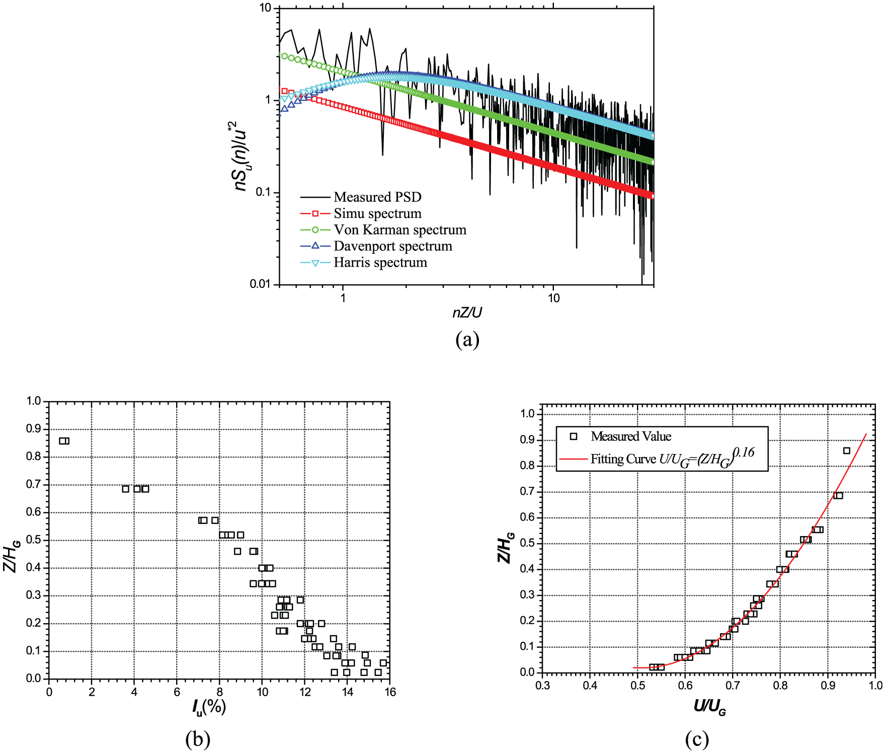
Simulation of Type B flow field in TJ-3 wind tunnel: (a) power-spectral function for along-wind component of wind speed; (b) turbulence intensity profile; and (c) average wind velocity profile.
The wind speed at the model top height is regarded as the reference wind speed, which is measured by a system composed of a pitot tube and a micromanometer. The wind pressures on the tower model are obtained using a pressure measurement system composed of a DSM3000 electronic pressure scanning valve, a PC machine, and a self-programming signal acquisition system, whose sampling frequency is 312.5 Hz. The data length at each pressure measurement point in each run is 6000. The 1:200 scaled pressure measurement model is made of synthetic glass, which ensures its strength and rigidity. Its prototype is a 235-m high cooling tower. 12 × 36 measurement points are arranged along the meridian and circumferential directions, respectively. The model in uniform and Type B flow fields are shown in Figure 2, and the distribution of the measurement points is presented in Figure 3.
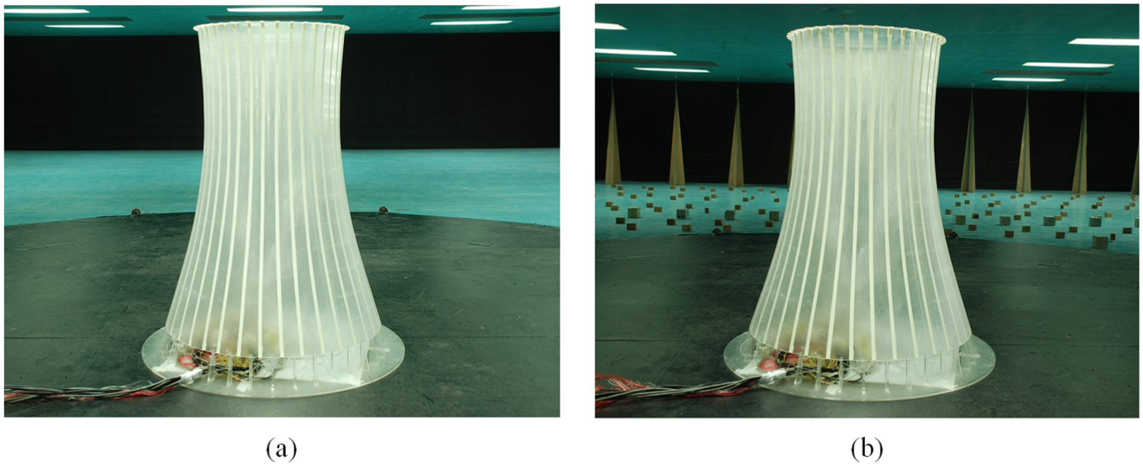
Tower model in two flow fields: (a) uniform flow field and (b) Type B flow field.
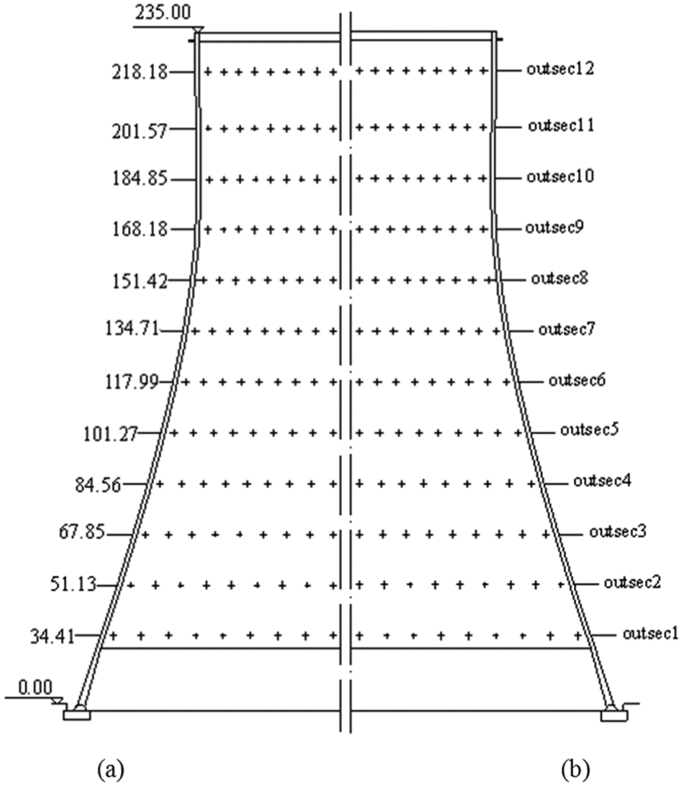
Measurement points on model surface and their prototype heights: (a) prototype heights (m) and (b) measurement sections.
To study the surface roughness effects, varied surface roughness is simulated on the model. The relative roughness k of the model is defined as follows (Simiu and Scanlan, 1996)
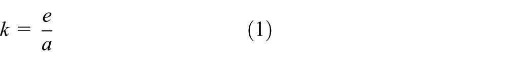
As shown in Figure 4, a corresponds to the rib spacing between the neighboring rough zones, b represents the width of the rough zone, and e is the thickness of the rough zone. Equation (1) does not take rib width b into account, because it has been found by Zou et al. (2015) that b does not have a significant influence on the wind pressure distributions when a is relatively small.
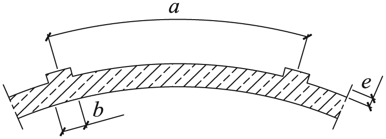
Schematic diagram of relative roughness definition.
The relative roughness for different simulations is listed in Table 1. As can be seen, there are eight surface roughness cases, whose relative roughness k ranges from 0 to 0.044. For each surface roughness case, pressure measurement tests in both uniform and Type B flow fields are conducted with 6, 8, 10, and 12 m/s wind speeds. The corresponding Re are 2.10 × 10⁵, 2.79 × 10⁵, 3.49 × 10⁵, and 4.19 × 10⁵, respectively. To avoid the end effects, the eighth circumferential section which is closest to the throat of the tower model is chosen as the characteristic section. Data obtained on the eighth section are processed using formulae listed in Appendix 1, and the results are given in the following subsections.
Relative roughness k for different cases.
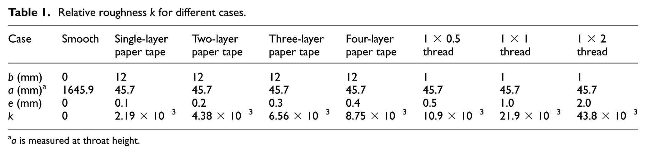
a is measured at throat height.
Mean wind pressure distribution
General results
Mean wind pressure distributions for different surface roughness cases are shown in Figure 5, which clearly demonstrates that surface roughness effects are extremely significant. As can be seen, the curves are gradually equalized with the increasing of surface roughness in general, and this general rule applies to almost all four wind speeds conditions in both uniform and ABL turbulent flow fields. The only exception is found for the condition of 6 m/s wind speed + uniform flow field, as the smooth and the single-layer paper tape surface roughness are not the worst cases in Figure 5(a). This should be attributed to the Re effects. Since the Re effects are greater for these two cases than for other cases in Figure 5(a) or cases in other subfigures according to section “Re effects on model test results,” the mean wind pressure distributions for these two cases probably deviate from their realities at high Re, breaking the general rule. In the following subsections, the static wind effect characteristic parameters are further identified from all the curves shown in Figure 5 (see Appendix 1 for their definitions), and the surface roughness effects on these parameters are meticulously studied.
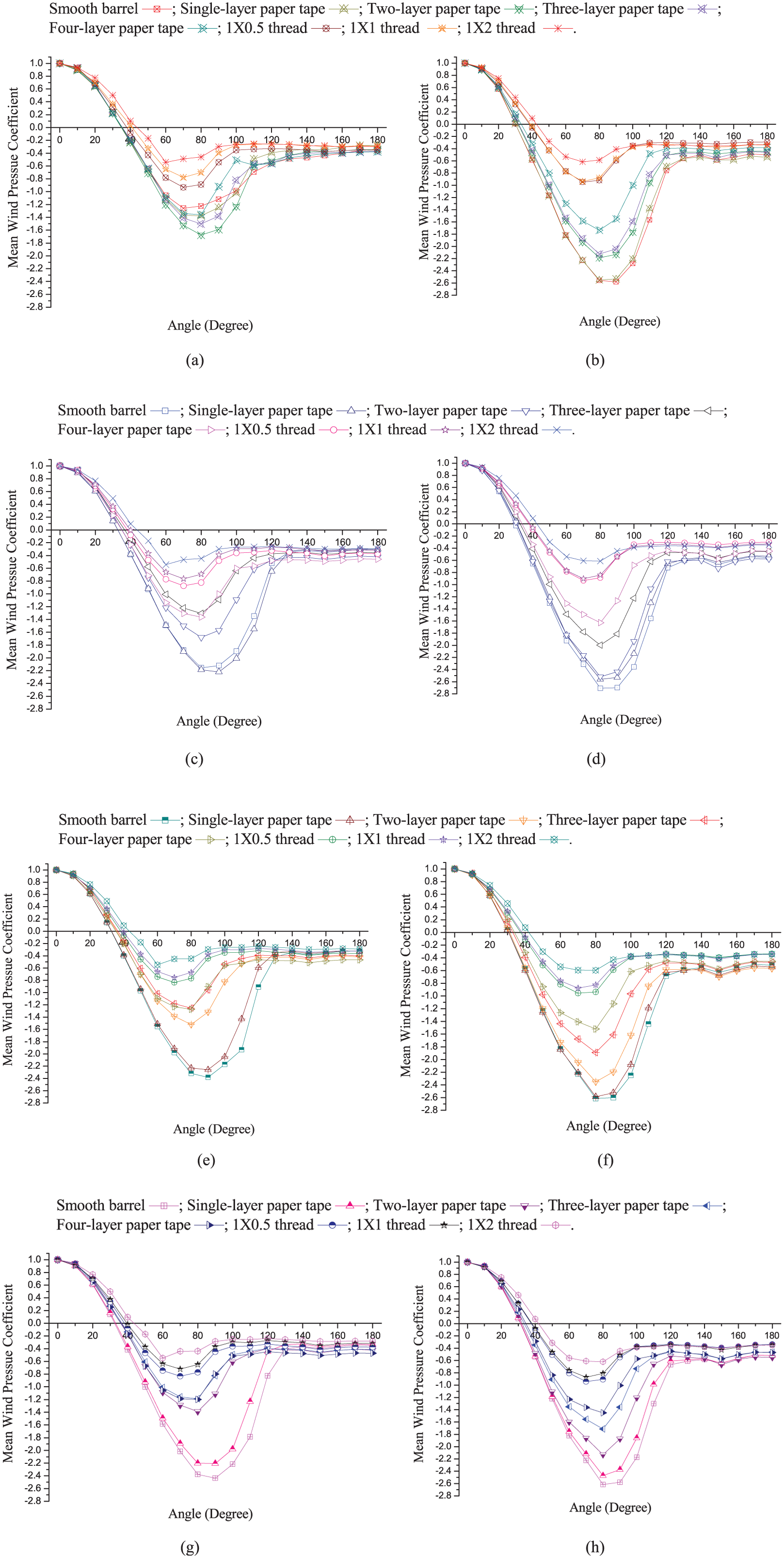
Mean wind pressure distributions on tower model with different surface roughness: (a) uniform flow field,+6 m/s wind speed; (b) Type B flow field,+6 m/s wind speed; (c) uniform flow field,+8 m/s wind speed; (d) Type B flow field,+8 m/s wind speed; (e) uniform flow field,+10 m/s wind speed; (f) Type B flow field,+10 m/s wind speed; (g) uniform flow field,+12 m/s wind speed; and (h) Type B flow field,+12 m/s wind speed.
Detailed results obtained in uniform flow field
In uniform flow field, the corresponding angle for the minimum pressure coefficient θmin is in between 60° and 90°. The θmin is in a gradual decreasing trend with the increase in relative roughness k of the model (the angle changes from 90° to 60°). In the case of the 6 m/s wind speed, the angle is first increased and subsequently decreased, in which the turning point is shown in the position of the two-layer paper tape. In the case of the 8 m/s wind speed, the angle is also first increased and subsequently decreased, in which the turning point is shown in the position of the single-layer paper tape, as shown in Figure 6(a). At the same time, with the increase in k, the absolute value of the minimum pressure coefficient Cpmin is in a significant decreasing trend, and a relatively obvious turning point is found in the position of the two-layer paper tape in the case of 6 m/s wind speed, as shown in Figure 6(b). The influence of the relative surface roughness k of the model on the wake flow pressure coefficient Cpb in the protected area is relatively insignificant. The pressure coefficient of the wake flow is distributed within the range from −0.5 to −0.2. With the increase in k, the wake flow pressure coefficient Cpb shows a trend of first decreasing and subsequently increasing, wherein the turning point is found in the position of the four-layer paper tape, as shown in Figure 6(c). The flow separation angle θb is in between 90° and 140°, and θb is gradually decreased with the increase in k, as shown in Figure 6(d). The angle with a pressure coefficient of zero θ0 is in between 32° and 44°. As shown in Figure 6(e), the angle θ0 gradually increases with the increase in k, and the angle θ0 for all cases is greater than the θ0-standardized = 32°, which corresponds to the standardized value of Chinese Codes (Figure 28). According to the literatures of previous field measurements, θ0 ≈ 35°, θb ≈ 110°, θmin ≈ 70°, and the corresponding values of pressure coefficients for different actual large cooling towers are different.
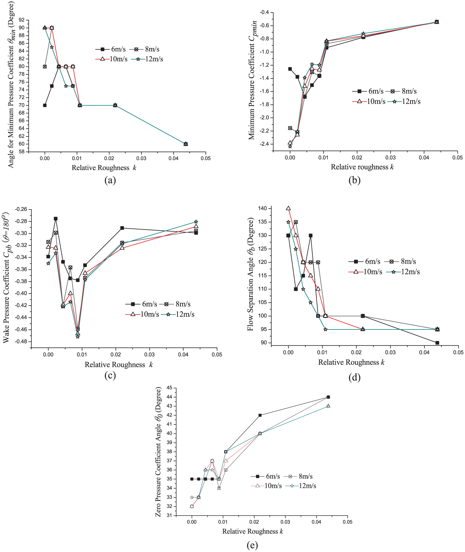
Influence of relative roughness on characteristic parameters of mean wind pressure distribution for uniform flow field: (a) θmin − k; (b) Cpmin − k; (c) Cpb − k; (d) θb − k; and (e) θ0 − k.
Besides, the influence of wind speed on the minimum pressure coefficient Cpmin is complicated. When the k value is small, the change in wind speed causes notable effects on the minimum pressure coefficient Cpmin. But with the increase in the k value, the influence of wind speed on the Cpmin is gradually reduced, as shown in Figure 6(b). The influence of wind speed on the corresponding angle for the minimum pressure coefficient θmin is similar to that on the Cpmin. When the k value is increased to a certain value, the influence of wind speed on θmin can be ignored, as shown in Figure 6(a). The changes in the wake flow pressure coefficient Cpb, the angle with a pressure coefficient of zero θ0, and the wake flow separation angle θb according to the increase in wind speed are more complicated, for which the overall trend is that the higher the wind speed and the greater the k value, the smaller the differences can be found among the Cpb, θb, and θ0 corresponding to different wind speeds, as shown in Figure 6(c) to (e), respectively.
Detailed results obtained in Type B flow field
In Type B flow field, the influence of the relative roughness k of the model on the circumferential distribution of the mean wind pressure coefficient around the characteristic section of the model is similar to that in uniform flow field. In Type B flow field, the corresponding angle for the minimum pressure coefficient θmin is in between 70° and 85°, and the θmin is in a gradual decreasing trend with the increase in the relative roughness, as shown in Figure 7(a). Same as in uniform flow field, the absolute value of the minimum pressure coefficient Cpmin significantly decreases with the increase in k in Type B flow field, as shown in Figure 7(b). The influence of the relative roughness k of the model on the wake flow pressure coefficient Cpb in the protected area in Type B flow field is more significant than that in the uniform flow field. The wake flow pressure coefficient is broadly distributed within the range from −0.6 to −0.28, and the wake flow pressure coefficient Cpb is shown in a slowly increasing trend with the increase in k. When k is greater than 0.011 (i.e. 1 × 0.5 thread case), Cpb tends to stabilize, as shown in Figure 7(c). The wake flow separation angle θb is in between 100° and 130°, and the angle with the pressure coefficient of zero θ0 is in between 28° and 42°. The θ0 is smaller compared with that in uniform flow field. With the increase in k, θb is shown in a gradually decreasing trend (see Figure 7(d)), and θ0 is shown in a gradually increasing trend (Figure 7(e)).
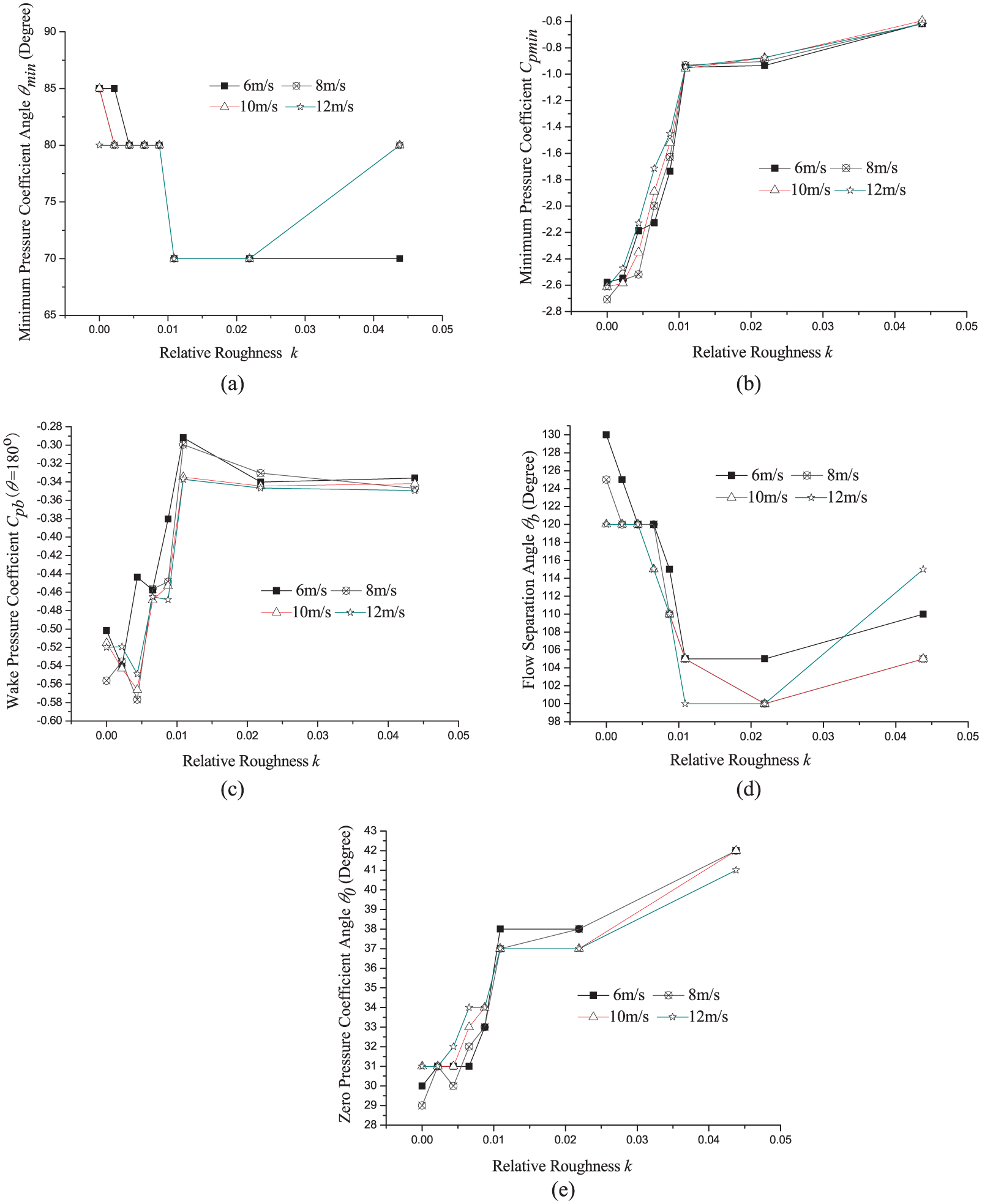
Influence of relative roughness on characteristic parameters of mean wind pressure distribution for Type B flow field: (a) θmin − k; (b) Cpmin − k; (c) Cpb − k; (d) θb − k; and (e) θ0 − k.
The influence of wind speed on the minimum pressure coefficient in Type B flow field is more complicated than that in uniform flow field. When the k value is very small or very large, the influence of the change of wind speed on the minimum pressure coefficient Cpmin is limited. But when k is in between 4.38 × 10⁻³ and 8.75 × 10⁻³, the influence of the change of wind speed on Cpmin is significant. The influence of wind speed on θb and Cpb is small, and there is basically no influence of wind speed on θ0 and θmin.
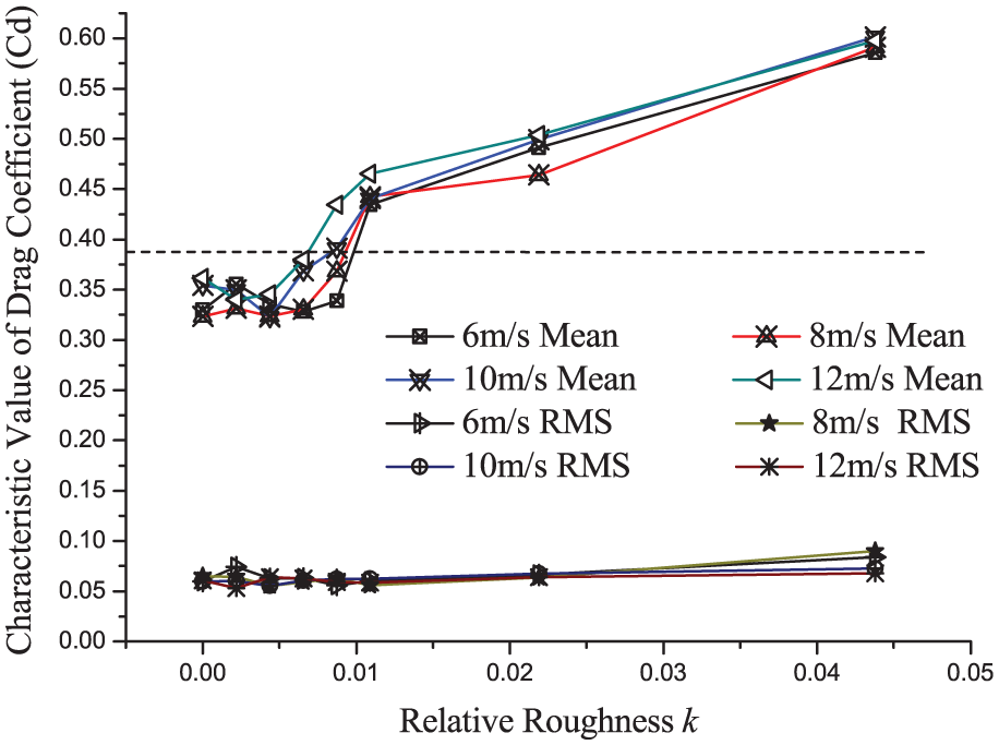
Drag coefficient
The drag coefficient calculated according to the standardized curve of Chinese Codes is 0.385, and the drag coefficient on the characteristic section of the tower model is changed with altered wind speed and surface roughness, as shown in Figures 8 to 11, respectively. In the uniform flow field, the influence of wind speed on the drag coefficient CD of the characteristic section is complicated. Within the wind speed range from 6 to 12 m/s, the smooth barrel case and the single-layer paper tape case are both in the transition area from the critical regime to the supercritical regime. The changes of the drag coefficient with the increase in wind speed for the three-layer paper tape case and the four-layer paper tape case are relatively large. The drag coefficients for the other four cases are relatively stable (Figure 8). With the increase in the relative roughness k of the model, CD gradually increases, and the trend is notable (Figure 10).
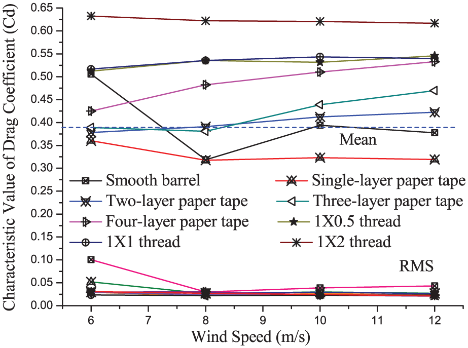
Drag coefficient: wind speed curves for uniform flow field.
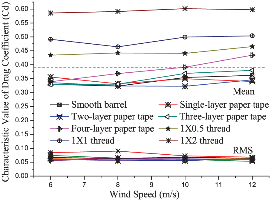
Drag coefficient: wind speed curves for Type B flow field.
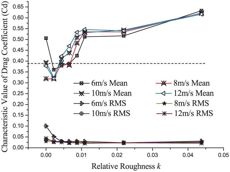
Drag coefficient: relative roughness curves for uniform flow field.
Drag coefficient: relative roughness curves for Type B flow field.
In Type B flow field, the change of the drag coefficient CD of the characteristic section with the increase in wind speed is not obvious (Figure 9). With the increase in relative roughness of the model, the drag coefficient CD of the characteristic section gradually increases, and the trend is more significant than that in the uniform flow field. Results indicate that the simulated flows around the model are out of the critical regime for all cases (Figure 11).
Fluctuating wind pressure distribution
As shown in Figure 12, in general, the intensities of the pressure fluctuations in side regions are obviously reduced with the increase in surface roughness for each flow condition. In uniform flow field, the fluctuating wind pressure distributions, or the circumferential distributions of the root mean square (RMS) value of pressure coefficient, can be roughly divided into three zones (Figure 12(a), (c), (e), and (g)). The first zone is from 0° to 25°, in which the RMS value of the pressure coefficient is relatively small. The RMS value of the pressure coefficient is basically constant with the increase in angle. The second zone is from 25° to 130°, in which flow separation occurs. In this zone, the RMS value of the pressure coefficient is first increased and subsequently decreased with the increase in angle. The RMS values thereof are obviously bigger than those of other zones and there are maximum values in the range from 80° to 110°. The RMS values for different relative roughness cases are of significant discrepancies from one another in this zone, and it is obvious that the larger the surface roughness, the smaller the RMS values are likely to be produced. The third zone is from 130° to 180°, in which the values are relatively constant and are slightly bigger than those of the first zone. For smooth barrel+6 m/s wind speed case and single-layer paper tape+6 m/s wind speed case, the RMS values of the pressure coefficients in the second zone and the third zone are notably larger than those for other cases. Generally, the wind speed has some influences on the RMS value of the pressure coefficient in uniform flow field, that is, the wind speed is approximately inversely proportional to the RMS value of the pressure coefficient.
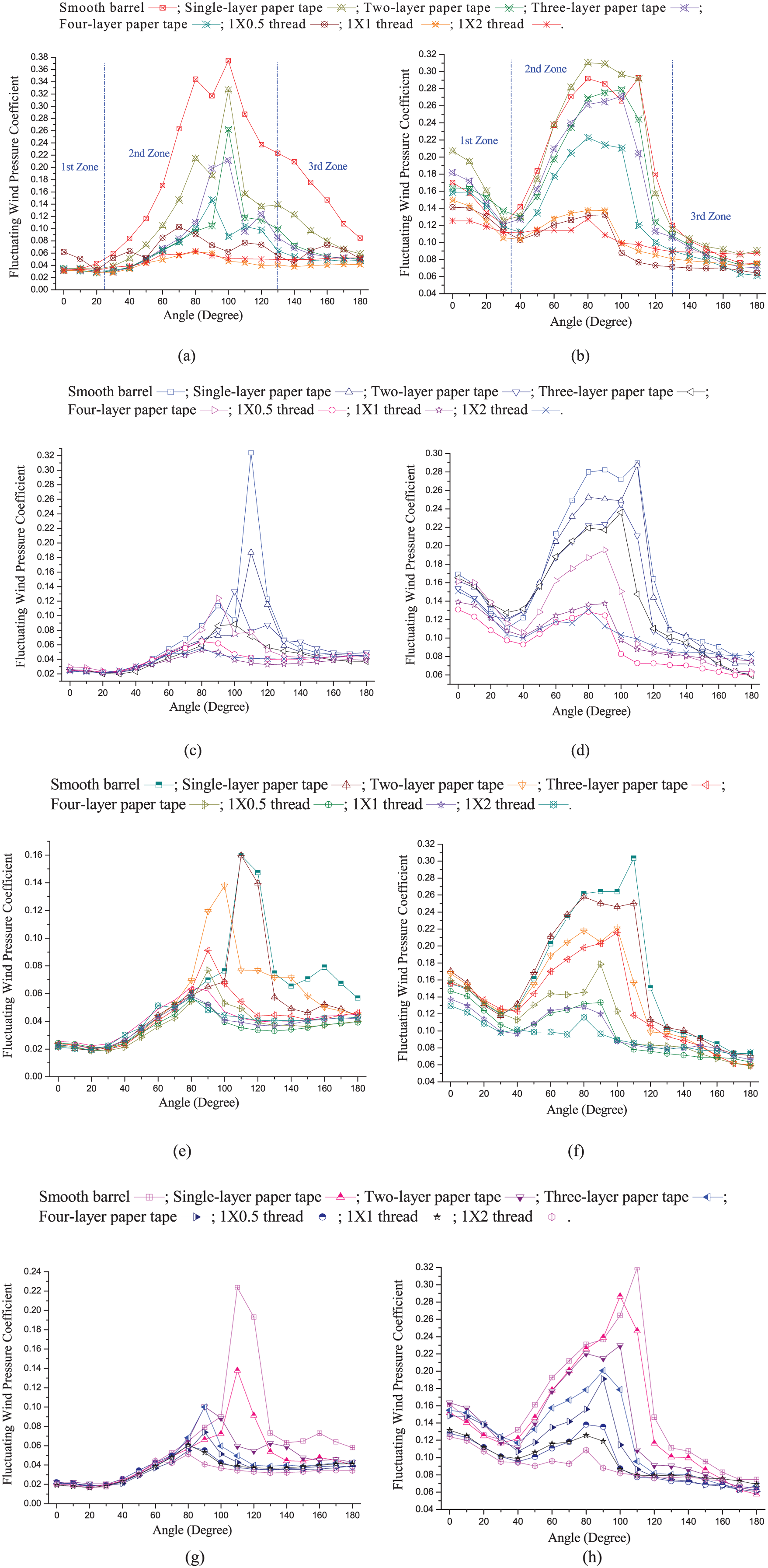
Fluctuating wind pressure distributions on tower model with different surface roughness: (a) uniform flow field,+6 m/s wind speed; (b) Type B flow field,+6 m/s wind speed; (c) uniform flow field,+8 m/s wind speed; (d) Type B flow field,+8 m/s wind speed; (e) uniform flow field,+10 m/s wind speed; (f) Type B flow field,+10 m/s wind speed; (g) uniform flow field,+12 m/s wind speed; and (h) Type B flow field,+12 m/s wind speed.
Similar to uniform flow field, the distribution of the RMS value of the pressure coefficient in Type B flow field can also be divided into three zones (Figure 12(b), (d), (f) and (h)). The first zone is from 0° to 35°, in which the RMS value of the pressure coefficient is relatively small, and the RMS value of the pressure coefficient is gradually decreased with the increase in the angle. The second zone is from 35° to some angle in between 110° and 130°, which is a flow separation zone. The RMS value of the pressure coefficient is first increased and subsequently decreased with the increase in angle in this zone, producing a maximum value in the position of around 90°. The discrepancies of RMS values among different surface roughness cases in this zone are also extremely large, and the phenomenon can be observed that the RMS values decrease with the increase in relative roughness in this zone. The third zone is from an angle in between 110° and 130° to 180°, in which the RMS value of the pressure coefficient continuously decreases with the increase in the angle, but the decreasing rate tends to be reduced. The RMS values in the third zone are smaller than those in the first zone.
In uniform flow field, the shapes of fluctuating wind pressure distributions around the throat section of the tower model are slightly rising slopes with sharp crests in the second zone. However, in Type B flow field, the shapes are slightly descending slopes with big obtuse crests in the second zone.
Strouhal number
With the increase in surface roughness on the model, the St is shown in the trend of first increased and subsequently stabilized for both uniform flow field and Type B flow field, as shown in Figure 13. The influence of wind speed on St is significant when k is relatively small. When the relative roughness of the model is increased to the value of 0.011, the sensitivity of St to the wind speed is significantly reduced. In uniform flow field, the maximum St is 0.147 for the case of three-layer paper tape +12 m/s wind speed, and in Type B flow field, the maximum St is 0.177 for the case of four-layer paper tape +6 m/s wind speed. They correspond to 0.031 and 0.037 Hz vortex shedding frequency, respectively in full scale (the oncoming flow velocity is assumed to be 22 m/s according to Chinese Codes). Since these vortex shedding frequencies are much lower than the fundamental natural frequencies of large cooling towers (greater than 0.7 Hz in general), there is no danger of vortex-induced resonance at all.
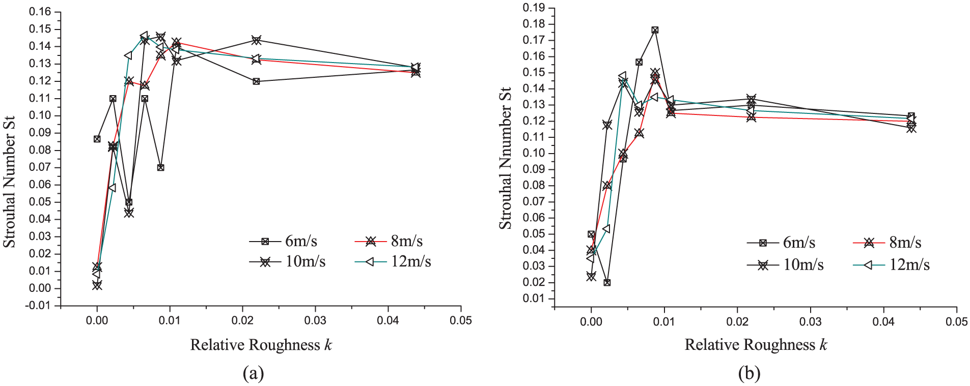
St for flow around tower model with different surface roughness: (a) uniform flow field and (b) Type B flow field.
Full-scale measurements
Studies using the wind tunnel model test are generally considered less reliable than those based on the full-scale measurement due to many similarity problems (inadequate simulation of small-scale turbulence content in ABL in the wind tunnel, the differences in stationary states of the wind flow for the two cases, Jensen number effects, and so on). In this section, our field measurement for wind pressures on the 167-m high Peng-cheng cooling tower is introduced. Some results are compared with those of early field measurement campaigns in history to validate the study described in section “Wind tunnel model test.”
Early full-scale measurement campaigns
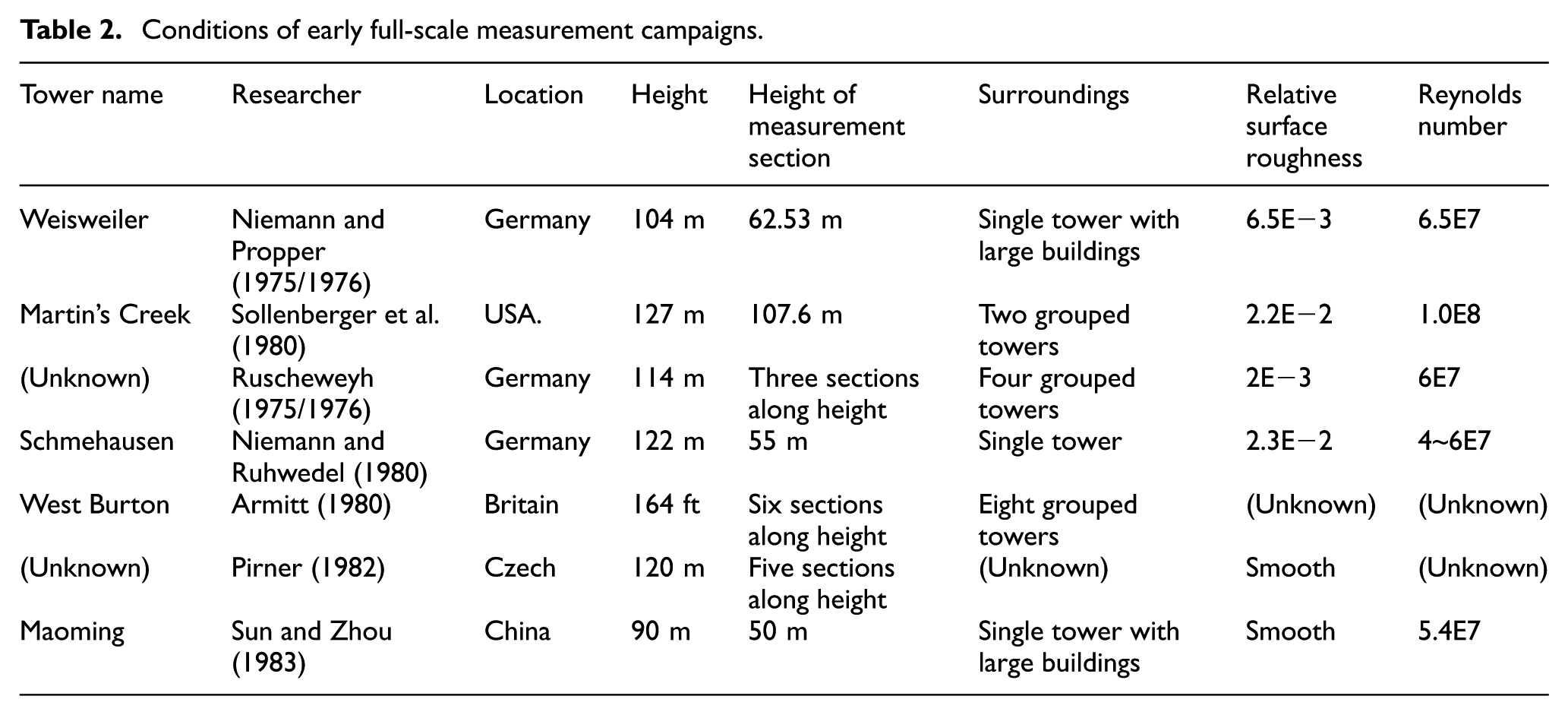
To obtain realistic wind effects on large cooling towers, some significant full-scale measurement campaigns were launched before 1985. Their engineering backgrounds are 104-m ribbed Weisweiler cooling tower (Niemann, 1971), 130-m ribbed Martin’s Creek cooling tower (Sollenberger and Scanlan, 1974), 122-m ribbed Schemehausen cooling tower (Niemann and Ruhwedel, 1980), and 90-m ribless Maoming cooling tower (Sun and Zhou, 1983). The specific conditions of all early full-scale measurement campaigns are listed in Table 2.
Conditions of early full-scale measurement campaigns.
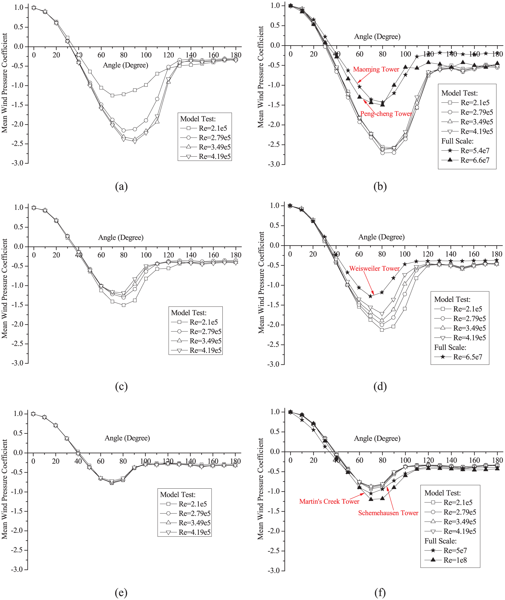
These early studies all pay attention to the mean wind pressure distribution, and the results obtained on these towers’ test throat sections are compared in Figure 14. It can be seen from Figure 14 that the patterns for the three ribbed cooling towers are close, although their relative roughness values are different from one another. However, the distribution of the smooth-walled Maoming cooling tower is remarkably different from those of rough-walled cooling towers. First, the minimum pressure coefficient of Maoming cooling tower is 0.2 smaller than those of others. Second, the wake flow pressure coefficient of Maoing cooling tower is 0.3 larger than those of others. These qualitatively agree with the conclusion drawn for the wind tunnel model tests (see section “Mean wind pressure distribution”).
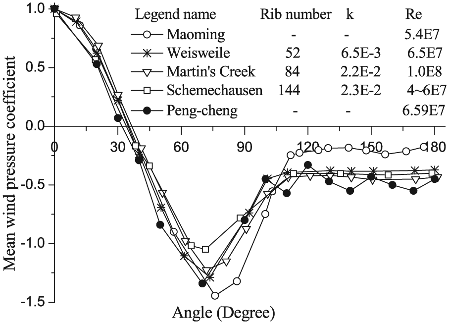
Mean wind pressure distributions on full-scale cooling towers.
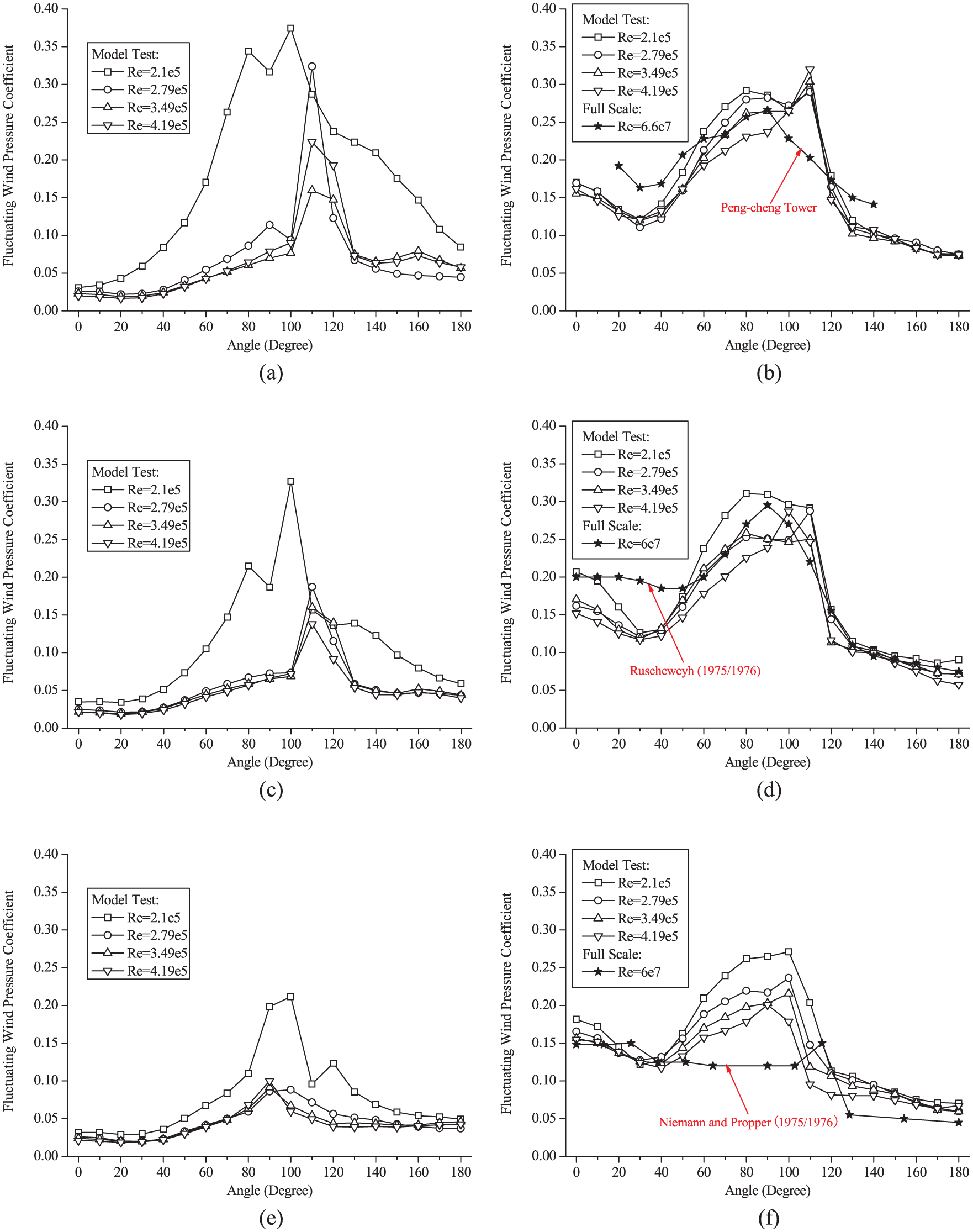
On the other hand, fewer field measurement campaigns pay attention to the full-scale fluctuating wind pressure distribution. The related result that can be found in an archival document is given by Ruscheweyh (1975/1976), who conducted full-scale measurements on a 114-m rough-walled cooling tower (k = 2E−3). Since there is no related research on smooth-walled cooling towers, comparison cannot be made to quantify the surface roughness effects on fluctuating wind pressure distribution at high Re for now. In this regard, a new field measurement campaign is launched, whose objective is to obtain the fluctuating wind pressure distribution on a full-scale smooth-walled cooling tower.
Setup for full-scale measurements
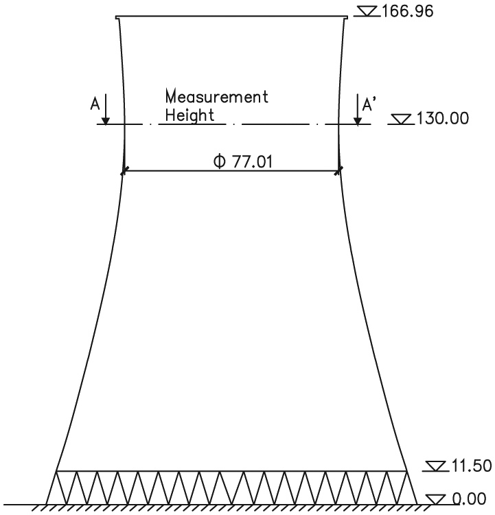
A 167-m smooth-walled cooling tower located in Peng-cheng power station, Xu-zhou, China is chosen for field measurements. To its south, there is an adjacent cooling tower same size as the one for measurements, and there is an industrial complex to its west (Figure 15). However, to its north and east, there is no large interfering building. During its construction, 36 transducers are evenly installed around the tower’s throat section at 130-m high (Figures 16 and 17). Besides, another transducer is arranged inside a cabin, which provides static reference pressure for measurements presented in this article.
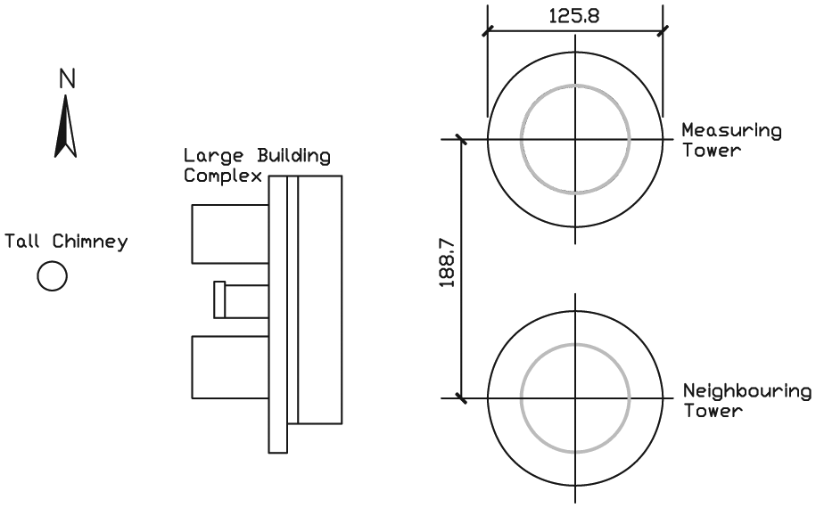
Site plan of Peng-cheng electric power station (m).
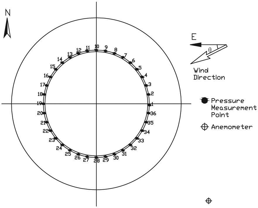
Plan of pressure measurement points.
Projection of measuring tower (m).
The wind pressure transducers used are piezoresistive ones, whose dimensions are as follows: 13 cm in length, 5 cm in width, and 3 cm in depth (Figure 18). The transducers’ maximum measured value is ±2.5 kPa (corresponding to 63 m/s wind speed). Their maximum sampling frequency and precision are 100 Hz and 1/1000 maximum range, respectively.
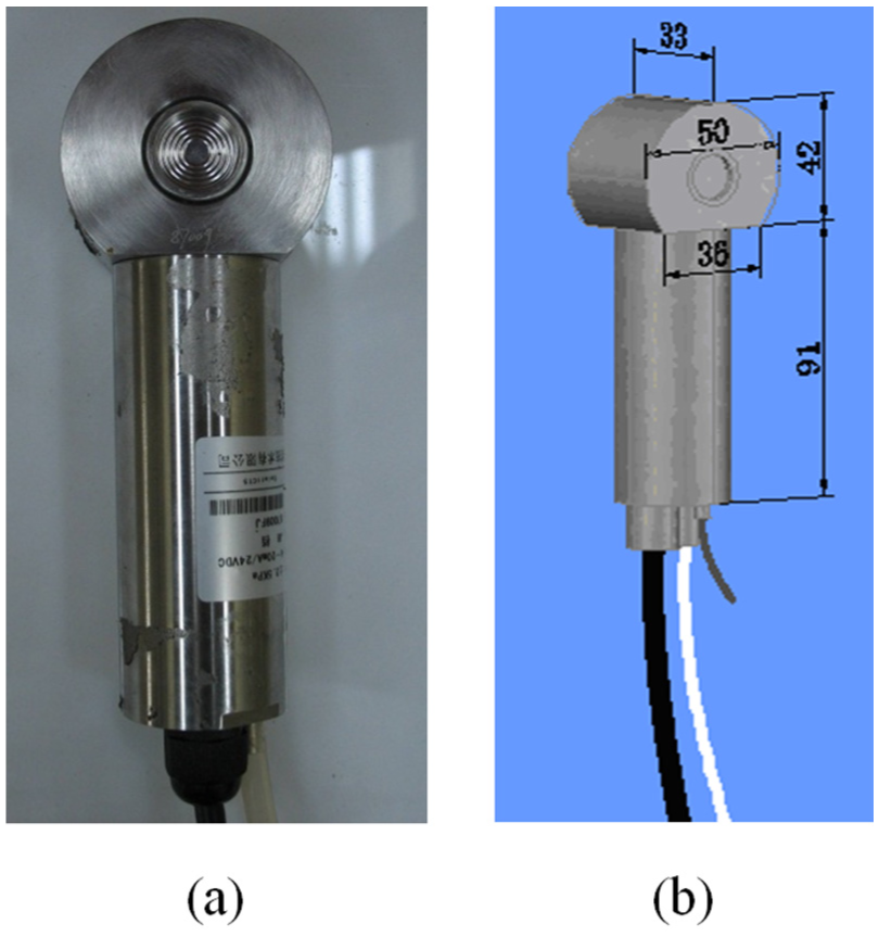
Wind pressure transducer: (a) an actual transducer and (b) dimension (mm).
Before installed on the prototype tower, the transducer is tested in TJ-2 wind tunnel of Tongji University for its performances. It is found that when oncoming flow speed is greater than 15 m/s, the noise-to-signal ratio for the transducer is kept below 5% (Figure 19(a)). Besides, it is shown that the signal produced by the transducer agrees with those obtained using high-precision electronic pressure scanivalve in 0–6 Hz frequency domain (Figure 19(b)). These prove that both static and dynamic performances of the transducer are agreeable.
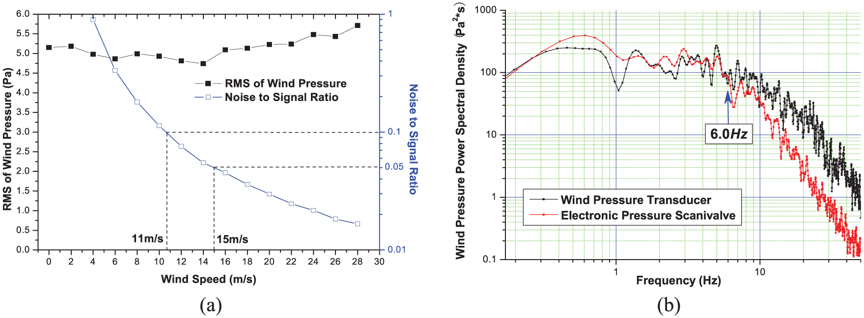
Wind tunnel tests for transducer’s performances: (a) static performance and (b) dynamic performance.
Oncoming flow measurements
Wind speed and wind direction are recorded by a two-dimensional (2D) propeller anemometer and a three-dimensional (3D) ultrasonic anemometer located to the southeast of the measuring tower at 20-m height (see Figure 20, also see Figure 16 for anemometers’ location in plan). For the 2D propeller anemometer, measured data are wind speed and wind direction in the horizontal plane. The 3D ultrasonic anemometer can record full oncoming flow information, including wind speed, azimuth angle, and elevation angle, which is more preferable in use under normal weather conditions. However, the performance of the 3D anemometer is likely to be adversely affected by rainwater. In this regard, 2D anemometer can be used as 3D anemometer’s substitute on rainy days.
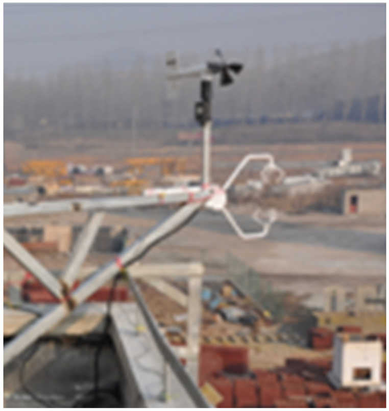
Anemometers.
The whole full-scale measurement campaign lasts from 2010 to 2015 on a 2–3 times of intensive tests per year basis. In each time, the occurrence of the strong wind scenario is predicted based on a local meteorological center’s weather forecast. Equipment are set up before the arrival of the strong wind, and 24-h simultaneous recordings for wind and wind-induced pressures are then conducted which usually continue for 1–2 weeks long. In the huge amount of data measured, those obtained from 28 November 2011 to 12 December 2011 are found to be most representative.
The predominate wind direction and the 10-min mean wind velocity obtained from 28 November to 12 December 2011 are shown in Figures 21 and 22, respectively (the mean wind velocities are obtained at 20-m high and converted to the corresponding values at130-m high using the power law formula of mean wind profile). As can be seen from Figure 22, only wind speeds for 29 November and 8 December exceed 12 m/s, which represent valid strong wind scenarios. However, the wind directions on the 2 days are quite different. On 29 November, the oncoming flow is from due east, but it is from due north on 8 December (Figure 21). Since some transducers installed on the tower’s north surface are found ineffective, complete fluctuating wind pressure distribution can only be obtained on 29 November. Besides, the upstream terrain is smooth, and there are no obvious interference effects caused by neighboring cooling towers or buildings with respect to the specific wind direction of 29 November. As a result, the wind-induced pressures recorded on 29 November 2011 should be used.
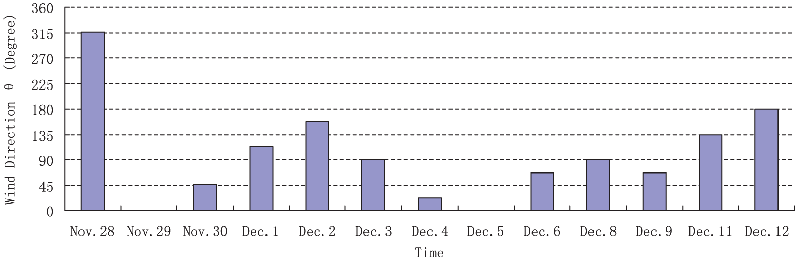
Predominant wind direction (see Figure 16 for definition of wind direction).
Converted 10-min mean wind speed at measurement height.
Results
In China, meteorological data in weather stations and regulations regarding wind loading used in Codes of Practice are given in period of 10 min. Hence, the long-term wind pressure records obtained on 29 November are divided into many 10-min data segments, and they are then processed separately using equations (2), (4), and (5) to give many mean/fluctuating wind pressure distributions. A representative mean wind pressure distribution obtained on Peng-cheng cooling tower is compared with the results of early full-scale measurement campaigns in Figure 14, which shows that they are both close.
Besides, six representative sets of fluctuating wind pressure distribution obtained are presented in Figure 23. Seemingly, no clear rules can be found from the scattered data shown in Figure 23. But, if abnormal data are abandoned (e.g. those at the angle of 100°), and curve fitting is executed to the rest of the data, a distribution similar to those obtained from wind tunnel model tests with Type B flow field (see section “Fluctuating wind pressure distribution”) is produced (the blue curve in Figure 23).
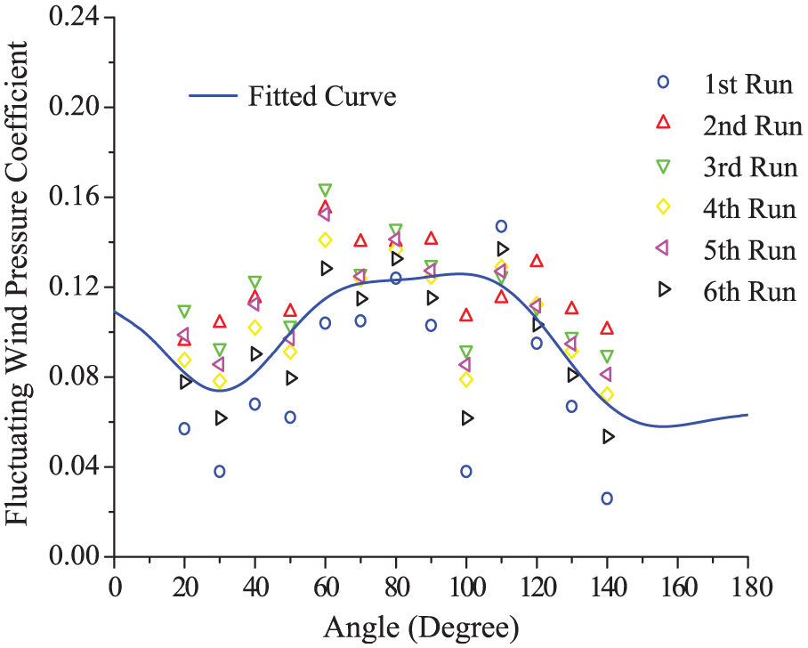
Fluctuating wind pressure coefficients for six runs.
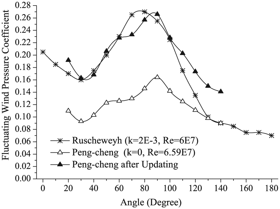
A representative fluctuating wind pressure distribution obtained on Peng-cheng cooling tower is selected and compared to Ruscheweyh’s result (Figure 24). It can be seen from Figure 24 that the fluctuating wind pressure coefficients obtained on the smooth-walled cooling tower are much smaller than those on the rough-walled cooling tower. This phenomenon disagrees with that observed in the wind tunnel model test (see section “Fluctuating wind pressure distribution”). However, a fact should be taken into account that the test section on Peng-cheng cooling tower is 130-meter high, which is much higher than that of Ruscheweyh’s test (91 m). And it has been found that the difference in test section height results in the discrepancy of the oncoming flow turbulence intensity, which in turn can cause significant effects on the fluctuating wind pressure distribution (Cheng et al., 2015). For a more reasonable comparison, updating of the fluctuating wind pressure coefficients obtained on Peng-cheng cooling tower is indispensable.
Fluctuating wind pressure distributions on full-scale cooling towers.
The updating procedures are as follows: (1) The fluctuating wind pressure coefficients measured on Peng-cheng cooling tower are fitted based on an eight-termed Fourier series formula, and the fluctuating wind pressure coefficient at stagnation is obtained from the fitted curve; (2) The fluctuating wind pressure coefficient at stagnation for Peng-cheng cooling tower (
Comparing Ruscheweyh’s fluctuating wind pressure distribution to the updated distribution for Peng-cheng cooling tower, Figure 24 shows that they basically agree in view of both pattern and magnitude. But the coefficients of smooth-walled Peng-cheng cooling tower seem larger than those of Ruscheweyh at windward and wake flow regions. This feature does not agree well with the result obtained from wind tunnel model tests (see section “Fluctuating wind pressure distribution”).
Re effects on model test results
It is widely acknowledged that the Re has significant impact on wind effects on circular cylinders, which can be proved by the fact that the drag coefficient obtained on a smooth-walled cylinder in uniform streams varies with the increase in Re (Achenbach, 1968; Roshko, 1961). Since the difference in Re between our wind tunnel model tests and actual scenarios for the large cooling tower is approximately three orders of magnitude, the similarity problem of the model tests deserves our attention.
Fortunately, Shih et al. (1993) found that wind effects on some rough-walled circular cylinders did not change with the increase in Re within the range Re ≈ 2 × 10⁵∼1 × 10⁷, which is called Re-independence range. By comparing the model test results obtained in the low-turbulence uniform flow field to those obtained in the ABL turbulent flow field in this article, it is proved that increased oncoming flow turbulence can also set up the phenomenon of Re-independence. These findings are presented in this section, which can help us make a fair judgment on the veracity of the model test results obtained in section “Wind tunnel model test.”
Re-independence range induced by increased surface roughness
Shih et al. (1993) conducted experiments on a circular cylinder in uniform flow field in a pressurized wind tunnel, whose results demonstrate that the greater the relative surface roughness is, the less significant the Re effects on the drag coefficient become within the range Re ≈ 2 × 10⁵∼1 × 10⁷ (Figure 25). Since the minimum relative surface roughness required to cause Re-independence is around k ≈ 0.01 (Figure 25), some results obtained in uniform flow field in section “Wind tunnel model test” might be inapplicable to the full-scale condition.
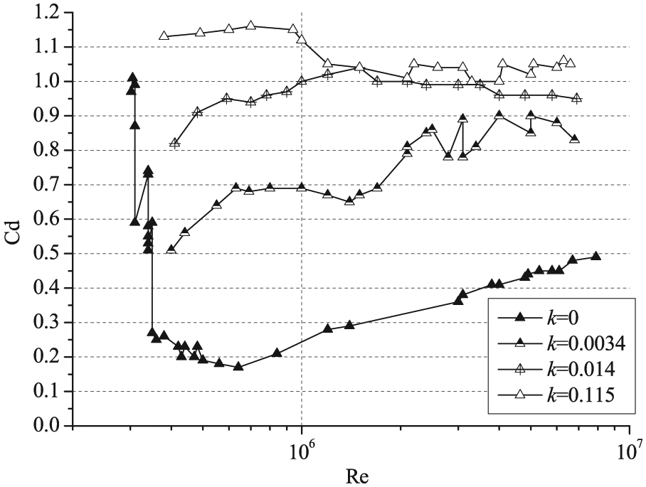
Re–CD curves for different surface roughness cases (reprinted from Shih et al. (1993)).
Re-independence range induced by increased oncoming flow turbulence
Some representative mean/fluctuating wind pressure distributions obtained in section “Wind tunnel model test” are categorized according to the flow field and the model surface roughness used, as shown in Figures 26 and 27, respectively. Comparing Figure 26(a), (c), and (e) or comparing Figure 27(a), (c), and (e), it can be found that the mean/fluctuating wind pressure distributions at different Re get closer to each other with the increase in relative surface roughness in uniform flow field, which is supportive to the finding of Shih et al. (1993). On the other hand, it can be found by comparing Figure 26(a) and (b), Figure 27(a) and (b), or Figure 27(c) and (d) that with increased oncoming flow turbulence intensity, the wind effects obtained on the tower model also become less dependent on Re. This observation is supported by Bearman (1968), Kiya et al. (1982), and Cheung and Melbourne (1983).
Mean wind pressure distribution: (a) smooth-walled cooling tower in uniform flow field; (b) smooth-walled cooling tower in Type B flow field; (c) rough-walled cooling tower (k = 0.0065) in uniform flow field; (d) rough-walled cooling tower (k = 0.0065) in Type B flow field; (e) rough-walled cooling tower (k = 0.022~0.023) in uniform flow field; and (f) rough-walled cooling tower (k = 0.022~0.023) in Type B flow field.
Fluctuating wind pressure distribution: (a) smooth-walled cooling tower in uniform flow field; (b) smooth-walled cooling tower in Type B flow field; (c) rough-walled cooling tower (k = 0.002~0.00219) in uniform flow field; (d) rough-walled cooling tower (k = 0.002~0.00219) in Type B flow field; (e) rough-walled cooling tower (k = 0.0065) in uniform flow field; and (f) rough-walled cooling tower (k = 0.0065) in Type B flow field.
Some field measurement results are also included in Figures 26 and 27 (see section “Full-scale measurements” for their backgrounds). In Figure 26(d) and (f) and Figure 27(b) and (d), the static/dynamic wind effects obtained from wind tunnel model tests are almost the same as those from full-scale measurements at high Re, indicating that the Re-independence induced by increased oncoming flow turbulence exists in a broad Re range. In Figures 26(b) and 27(f), there are some differences between full-scale measurement and model test results, which are probably caused by the fact that the static reference pressure established for the full-scale measurement can hardly play the same role as the static pressure in the wind tunnel. In sum, Re-independence range induced by increased oncoming flow turbulence intensity exists in Re ≈ 2 × 10⁵∼1 × 10⁸, so Re effects on all results obtained in Type B flow field in section “Wind tunnel model test” are limited.
Conclusion
The findings of this study concerning the wind effects on rough-walled and smooth-walled large cooling towers are summarized as follows:
It is found by wind tunnel model tests that the magnitude of negative mean wind pressure coefficients and the intensity of the pressure fluctuations at side regions both decrease remarkably with the increase in surface roughness, which supports the use of ribs on prototype large cooling towers for the purpose of reducing mean/extreme side suctions. Field measurement results at high Re are employed to validate this conclusion drawn from wind tunnel model tests. Comparison of the mean wind pressure distributions obtained on rough-walled and smooth-walled full-scale cooling towers is supportive of the model test result. However, comparison of the fluctuating wind pressure distributions obtained at high Re does not quite support the model test result. The causes of the discrepancy between full-scale and model test results probably are as follows: (1) the static reference pressure established for the full-scale measurement might hardly play the same role as the static pressure in the wind tunnel; (2) the full-scale velocity field lacks stationarity and homogeneity as compared with the wind tunnel situation; 3) simulation of small-scale turbulence content in ABL in the wind tunnel is inadequate.
The model test results for the ABL turbulent flow field are obtained in the range of Re-independence, which can be used for improving Chinese Codes and other countries’ Codes of Practice which currently do not support the design of ribbed cooling towers. Comparing the model test results for the low-turbulence uniform flow field to those for the ABL turbulent flow field, it is found that they qualitatively agree. However, when quantitative study becomes the aim, most results obtained in the uniform flow field are not likely to be applicable to the prototype structure since Re effects on those results are significant.
Although this article proves that increased surface roughness leads to reduced wind effects on cooling towers, it is found that a limit of relative roughness exists at k ≈ 0.01. When k is greater than that limit, the helpful effects of increased surface roughness diminish.
Footnotes
Appendix 1
Appendix 2
Declaration of Conflicting Interests
The author(s) declared no potential conflicts of interest with respect to the research, authorship, and/or publication of this article.
Funding
The author(s) disclosed receipt of the following financial support for the research, authorship, and/or publication of this article: The authors gratefully acknowledge the supports of the National Natural Science Foundation of China (51178353 and 50978203), the National Key Basic Research Program of China (i.e. 973 Program) (2013CB036300), and the Kwang-Hua Fund for the College of Civil Engineering, Tongji University.