Verification of probability density evolution method through shaking table tests of a randomly base-driven structure

Abstract

Over the last decade, a family of probability density evolution method for analysis of general stochastic dynamical systems has been developed. A large number of numerical examples indicate that this method has advantages in quantification of stochastic dynamic response, in assessment of global reliability and in stochastic optimal control of structures, while its experimental verification is still lacking. The main purpose of this article, with the consequence, is to experimentally investigate the accuracy and efficiency of the probability density evolution method through shaking table tests of a randomly base-driven structure. Analytical results demonstrate that the probability density evolution method is capable of evaluating the probability information, including the mean, the standard deviation, the instantaneous probability density function and its evolution, of structural responses exactly. Furthermore, stochastic response analyses of the tested structure without dampers subjected to three different sets of ground motions are conducted to validate the correctness and reliability of the probability density evolution method. It is concluded that a small amount of representative samples is able to accommodate a relatively accurate analytical result of stochastic dynamical systems, indicating a significant efficiency of the probability density evolution method.

Keywords

Experimental verification numerical validation probability density evolution method representative samples shaking table tests

Introduction

Traditional analysis of dynamic response of structures, only conducting its deterministic counterpart in most cases, has been studied in depth (Chopra, 2011; Clough and Penzien, 1993). Dynamical systems, however, essentially exhibit appreciable randomness, including that comes from initial conditions, from external excitations and from system parameters. As a result, the uncertainty involved in those systems may lead to a considerable random fluctuation of dynamic responses (Li and Chen, 2009). Thus, stochastic dynamic response analysis, considering the randomness of dynamical systems, is of paramount importance in structural engineering, especially in practical applications.

Thanks to many efforts devoted to stochastic dynamics of structures, there have been extensive developments in this discipline, such as the random vibration theory, the approaches for analysis of structures with random parameters, and so on. Because of finite precision measurements of system status, uncertainties are usually unavoidable in initial conditions. For such kind of systems, the probability density function (PDF) of status is governed by the Liouville equation (Kozin, 1961; Syski, 1967). For the systems involving stochastic dynamic excitations, see earthquakes, strong winds, and sea waves, the response analysis of linear structural systems can be completely treated based on the classical random vibration theory, which includes the correlation analysis, the spectral representation, the Fokker–Planck–Kolmogorov (FPK) equation approach, and the pseudo-excitation method (Lin and Zhang, 2004; Lutes and Sarkani, 2004). However, the stochastic response analysis of general nonlinear structural systems still remains a challenge despite years of endeavors (Lin and Cai, 1995; Zhu, 2003). In the case randomness arises in system parameters, say, the material properties, the geometrical parameters, and the boundary conditions, most analysis approaches, such as the Monte Carlo simulation, the perturbation method, and the orthogonal expansion method, were in attempt to capture the statistical quantities, while not the PDFs of structural responses (Ghanem and Spanos, 1991; Li, 1996). Furthermore, even as far as the second-order statistical quantities are concerned, effective approaches were unavailable for nonlinear structural systems before the early 21th century.

Over the last decade, a family of probability density evolution method (PDEM) has been developed for analysis of general stochastic dynamical systems (Li, 2016; Li and Chen, 2004, 2008, 2009; Li et al., 2012a). In this method, a generalized density evolution equation (GDEE) was derived according to the random event description of the principle of preservation of probability. It should be pointed out that the GDEE holds with regard to arbitrary physical quantities, such as displacements, accelerations, and stresses, associated with single-degree-of-freedom (SDOF)/multi-degree-of-freedom (MDOF) linear/nonlinear dynamical systems involving randomness coming simultaneously from initial conditions, external excitations, and system parameters. With the PDEM, a complete PDF description of system responses can be gained through integrating deterministic dynamic analysis and finite difference method. So far, the PDEM has been successfully applied to stochastic response analysis, dynamic reliability evaluation, and stochastic optimal control of structures (Chen and Li, 2007; Li and Chen, 2004; Li et al., 2007, 2010; Mei et al., 2013; Peng et al., 2014a, 2014b; Xu and Li, 2016).

Through comparative studies on the solutions of a MDOF system using the PDEM and Monte Carlo simulations, respectively, the former, proposed by Li and Chen, has been demonstrated by a large number of numerical examples (Chen and Li, 2007; Li and Chen, 2004; 2005a; 2005b, 2006a; Peng et al., 2014a). In this article, the focus is to experimentally investigate the accuracy and efficiency of the PDEM through shaking table tests of a randomly base-driven structure. In section “PDEM for analysis of stochastic dynamical systems,” a brief introduction of the PDEM as well as corresponding numerical implementation procedures is provided. Section “Stochastic seismic control experiments” details the experimental setup and experimental program relevant to complete shaking table tests of structures with and without dampers. In the experiments, a physical stochastic ground motion model is employed to generate the representative ground acceleration time histories, which are used as the inputs of shaking table. The verification of the PDEM based on the results of stochastic seismic control experiments is carried out in section “Verification of the PDEM based on results of stochastic seismic control experiments.” In order to further validate the correctness and reliability of the PDEM, section “Validation of the PDEM by numerical simulations” focuses on stochastic response analyses of the tested structure subjected to three sets of representative ground motions with different samples. The concluding remarks are included in the final section.

PDEM for analysis of stochastic dynamical systems

As mentioned above, the PDEM for general stochastic dynamical systems, including MDOF nonlinear structures involving random parameters and stochastic excitations, has been developed (Li, 2016; Li and Chen, 2004, 2008, 2009; Li et al., 2012a). In order to investigate the accuracy and efficiency of the PDEM based on the stochastic control experiments previously mentioned, in which only the randomness coming from seismic excitations is considered, a brief introduction of the PDEM and corresponding numerical implementation procedures is provided in this section.

Axioms of the PDEM

With discretization techniques such as the finite element method, the equation of motion of a structure subjected to earthquake ground motions reads

M \overset{\cdot\cdot}{X} + f (\overset{\cdot}{X}, X) = - M I {\overset{\cdot\cdot}{x}}_{g} (Θ, t), {\overset{\cdot}{X}}_{0} = {\overset{\cdot}{x}}_{0}, X_{0} = x_{0}

(1)

where $X = (X_{1}, X_{2}, \dots, X_{n})^{T}$ denotes n by 1 displacement vector; overdots denote differentiation with regard to t; M denotes n by n mass matrix; f denotes internal forces of the structures including the damping and restoring forces; I denotes a n-order column vector with all the components being 1; ${\overset{\cdot\cdot}{x}}_{g} (Θ, t)$ denotes the earthquake ground motion; and $Θ = (Θ_{1}, Θ_{2}, \dots, Θ_{s})$ denotes random vector characterizing the randomness involved in the ground motion. The joint PDF of $Θ$ is identified as $p_{Θ} (θ)$ . ${\overset{\cdot}{x}}_{0}$ , $x_{0}$ denote the initial velocity and initial displacement vectors, respectively.

It is evident that any arbitrary response of interest $X (t)$ depends upon $Θ$ and could be written in the form of a function as

X (t) = H ({\overset{\cdot}{x}}_{0}, x_{0}, Θ, t)

(2)

where $x_{0}$ denotes the initial value of $X (t)$ . Using the principle of preservation of probability, one can deduce the GDEE governing the joint PDF of $(X, Θ)$ (Li, 2016; Li and Chen, 2008, 2009; Li et al., 2012a)

\frac{\partial p_{X Θ} (x, θ, t)}{\partial t} + \overset{\cdot}{X} (θ, t) \frac{\partial p_{X Θ} (x, θ, t)}{\partial x} = 0

(3)

where $p_{X Θ} (x, θ, t)$ indicates joint PDF of $(X, Θ)$ ; $\overset{\cdot}{X} (θ, t)$ indicates the velocity of $X (t)$ under the condition ${Θ = θ}$ .

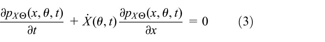
The initial condition for equation (3) reads

p_{X Θ} (x, θ, t) |_{t = 0} = δ (x - x_{0}) p_{Θ} (θ)

(4)

where $δ (\cdot)$ denotes Dirac’s delta function.

The joint PDF $p_{X Θ} (x, θ, t)$ could be given by solving the initial-value partial differential equations (3) and (4) using the numerical procedures (Li and Chen, 2008, 2009; Li et al., 2012a). The instantaneous PDF of $X (t)$ could be obtained by

p_{X} (x, t) = \int_{Ω_{Θ}} p_{X Θ} (x, θ, t) d θ

(5)

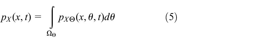
where $Ω_{Θ}$ indicates the distribution domain of $Θ$ .

Numerical implementation procedures for the PDEM

To get instantaneous PDFs or other probabilistic indices of responses, a set of equations, consisting of the motion equation (1), the GDEE (3) with the initial condition equation (4), and the integration in equation (5), are to be solved. For generally practical structures, these equations can be numerically solved by the following steps:

Select representative points $θ_{q} (q = 1, 2, \dots, N_{sel})$ in the domain $Ω_{Θ}$ , where $N_{sel}$ is the total number of the selected points. Discretize the initial condition equation (4) accordingly;

For the prescribed $Θ = θ_{q}$ , solve equation (1) with a deterministic time integration method to evaluate the value of $\overset{\cdot}{X} (θ_{q}, t_{m})$ , where $t_{m} = m D t (m = 1, 2, \dots)$ , Dt is the time step;

Introducing $\overset{\cdot}{X} (θ_{q}, t_{m})$ into the GDEE (3), solve equation (3) under the initial condition equation (4) with the finite difference method to give the numerical solution of $p_{X Θ} (x, θ, t)$ , denoted by $p_{X Θ} (x_{j}, θ_{q}, t_{k})$ , here $x_{j} = x_{0} + j D x (j = 0, \pm 1, \pm 2, \dots)$ , Dx is the space step, $t_{k} = k D t_{s}$ , Dt_s is the time step in the finite difference method;

Repeat steps 2 and 3 running over $q = 1, 2, \dots, N_{sel}$ , and then take numerical integration in equation (5) to compute the numerical solution of $p_{X} (x, t)$ .

It should be noted that the strategy of selecting representative points in step 1 has a great influence on the accuracy and efficiency of the PDEM. So far, several methods of selecting points, such as the mapping-based dimension-reduction technique, the strategy of selecting representative points via tangent spheres, and the number theoretical method, have been developed (Li and Chen, 2006b; 2007; Chen and Li, 2008). When selecting representative points, an appropriate strategy should be chosen according to the number of random parameters of systems. Moreover, it is seen from the steps detailed above that a traditional deterministic dynamic response analysis process is embedded in the procedure, which has been extensively studied (Chopra, 2011; Clough and Penzien, 1993). Additionally, the numerical methods for the partial differential equation (3), say, the finite difference method, are well developed in computational fluid dynamics (Anderson, 1995). As such, it is convenient to conduct a stochastic dynamic response analysis of structures according to the above procedures.

Stochastic seismic control experiments

Generation of representative ground motions

Based on the physical background, seismic ground motions are mainly affected by the properties of earthquake source, propagation path, and local site. The uncertainty of the three factors is the cause of the randomness of seismic ground motions. For a certain engineering site, the ground motion parameters at the bedrock could be provided by the seismic hazard assessment considering the properties of the sources and the propagation process (Dowrick, 2003; Wang and Li, 2011). Therefore, taking into account the properties of the site soil and combining with the ground motion at the bedrock will lead to the so-called physical stochastic ground motion model (Li and Ai, 2006).

Notice that the effects of engineering site could be regarded as a multi-layer filtering operator. For the sake of clarity, it is modeled as a SDOF system. Using the ground motion at the bedrock as the input process, the absolute response of the SDOF system is namely the process of the ground motion at the surface of the engineering site. Therefore, the physical stochastic ground motion model can be expressed in the frequency domain as (Li and Ai, 2006)

{\overset{\cdot\cdot}{X}}_{g} (Θ, ω) = H_{g} (Θ_{ω_{0}}, Θ_{ζ_{0}}, ω) \cdot {\overset{\cdot\cdot}{U}}_{b} (Θ_{b}, ω)

(6)

H_{g} (Θ_{ω_{0}}, Θ_{ζ_{0}}, ω) = \frac{Θ_{ω_{0}}^{2} + 2 i Θ_{ζ_{0}} Θ_{ω_{0}} ω}{Θ_{ω_{0}}^{2} - ω^{2} + 2 i Θ_{ζ_{0}} Θ_{ω_{0}} ω}

(7)

where ${\overset{\cdot\cdot}{X}}_{g} (Θ, ω)$ and ${\overset{\cdot\cdot}{U}}_{b} (Θ_{b}, ω)$ are the frequency domain expressions of ground motions at the engineering site and the bedrock, respectively. $Θ = (Θ_{ω_{0}}, Θ_{ζ_{0}}, Θ_{b})$ is the random parameter vector characterizing the randomness involved in the ground motion at the surface of the engineering site. Specifically, $Θ_{ω_{0}}$ , $Θ_{ζ_{0}}$ are the random parameters denoting the random nature of the site soil, that is, the predominant frequency of the engineering site $ω_{0}$ and the equivalent damping ratio $ζ_{0}$ , and $Θ_{b}$ is the random parameter characterizing the randomness involved in the ground motion at the bedrock. It is noted that the probability distributions of the three random parameters can be identified by introducing a large number of earthquake records. Identification results reveal that $Θ_{ω_{0}}$ , $Θ_{ζ_{0}}$ , and $Θ_{b}$ obey the lognormal distribution: the mean is 20 rad/s, 0.7, and 0.25 m/s^0.5, respectively; the coefficient of variation is 0.4, 0.3, and 0.5, respectively (Li and Ai, 2006). The time history of the stochastic ground motion could then be obtained by the inverse Fourier transformation

{\overset{\cdot\cdot}{x}}_{g} (Θ, t) = \frac{1}{2 π} \int_{- \infty}^{\infty} {\overset{\cdot\cdot}{X}}_{g} (Θ, ω) e^{i ω t} d ω

(8)

Employing the strategy of selecting representative points via tangent spheres (Chen and Li, 2008) and introducing the statistical information into equation (8), 120 representative ground accelerations are generated by means of the above physical stochastic ground motion model (Li and Ai, 2006). Meanwhile, the ground acceleration valued by the mean parameters is obtained, and its peak acceleration is 1.00 m/s². It is worth noting that the peak accelerations as well as the frequency spectrum characteristics of the representative ground accelerations differ from each other. The mean and standard deviation of peak accelerations of the 120 ground motions are 1.09 and 0.28 m/s², respectively. It is seen that the coefficient of variation of peak accelerations is up to 0.256. Moreover, the maximum value of peak accelerations of the 120 ground motions is 2.30 m/s², about 6 times the minimum value. Three typical ground accelerations, labeled W038, W064, W079, and their Fourier amplitude spectra are, respectively, shown in Figure 1. It is clear that the time and frequency domain characteristics of the typical ground accelerations are quite different. From the differences, one might understand the randomness involved in the seismic excitation. Besides, the ground acceleration generated using the mean parameters, labeled W000, and its Fourier amplitude spectrum are also pictured in Figure 1.

Figure 1.

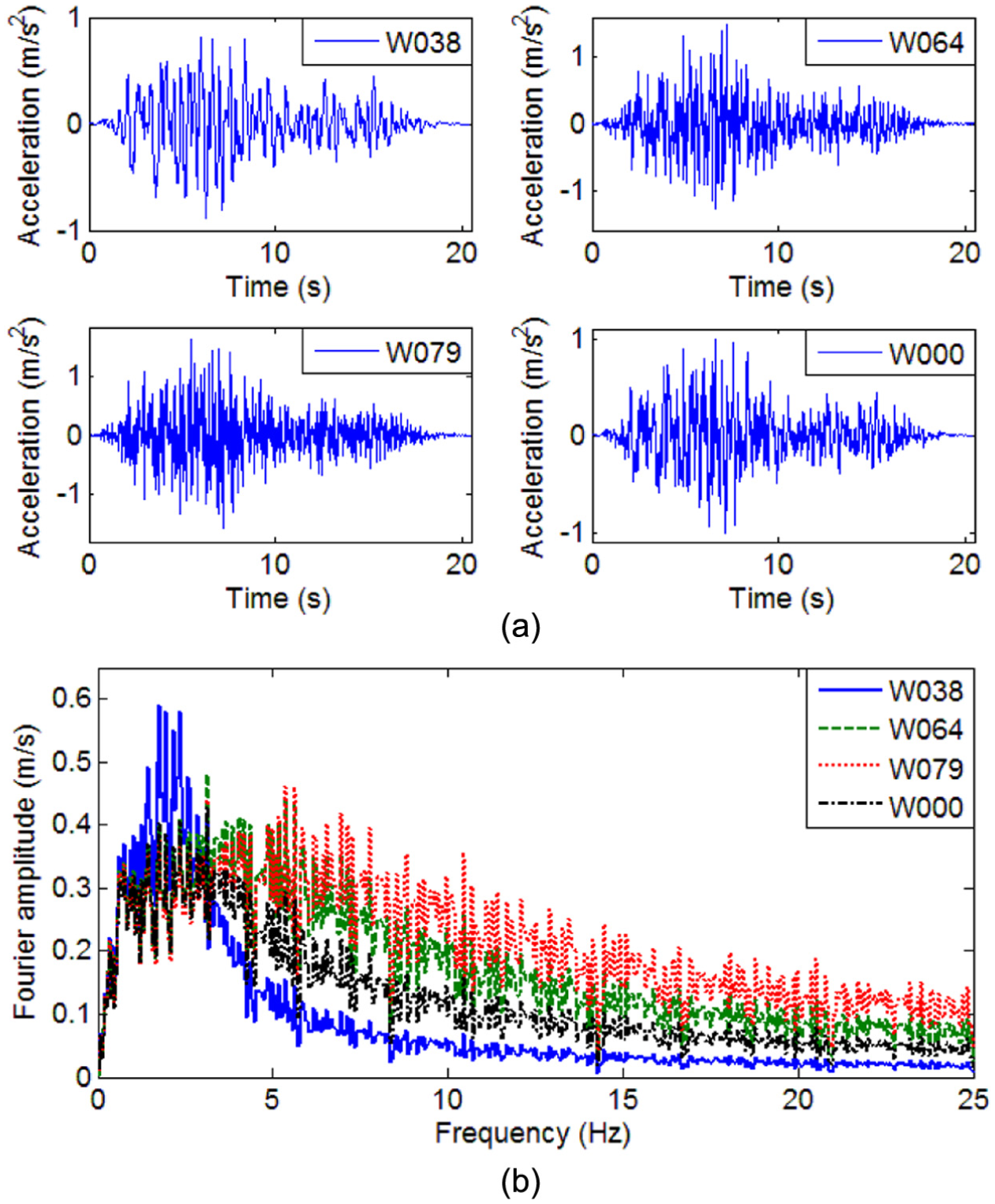
Typical time histories and Fourier amplitude spectra of ground accelerations: (a) time histories of ground accelerations and (b) Fourier amplitude spectra of ground accelerations.

Experimental setup

Experimental investigations were performed in the State Key Laboratory of Disaster Reduction in Civil Engineering at Tongji University, China. The experimental facility is a 4.0 m×4.0 m shaking table with a capacity of 2.5×10⁴ kg.

The tested model used in this experiment is a six-story and single-bay steel structure as shown in Figure 2(a). It is designed to be a 1/5-scale model of a part of a prototype steel structure. Overall dimensions of the model are 1.6 m×1.6 m in plane with story height of 1.0 m for the first story and 0.8 m for the other stories. Its total mass is about 10.0 ton which includes 7.2 ton artificial mass distributed evenly on the six floors allowing for the similar dynamic behaviors to the prototype structure (Li et al., 2012b; Mei et al., 2013; Peng et al., 2014b). The model-to-prototype ratios of time, force, mass, displacement, and acceleration are 0.4472, 0.04, 0.04, 0.2, and 1, respectively.

Figure 2.

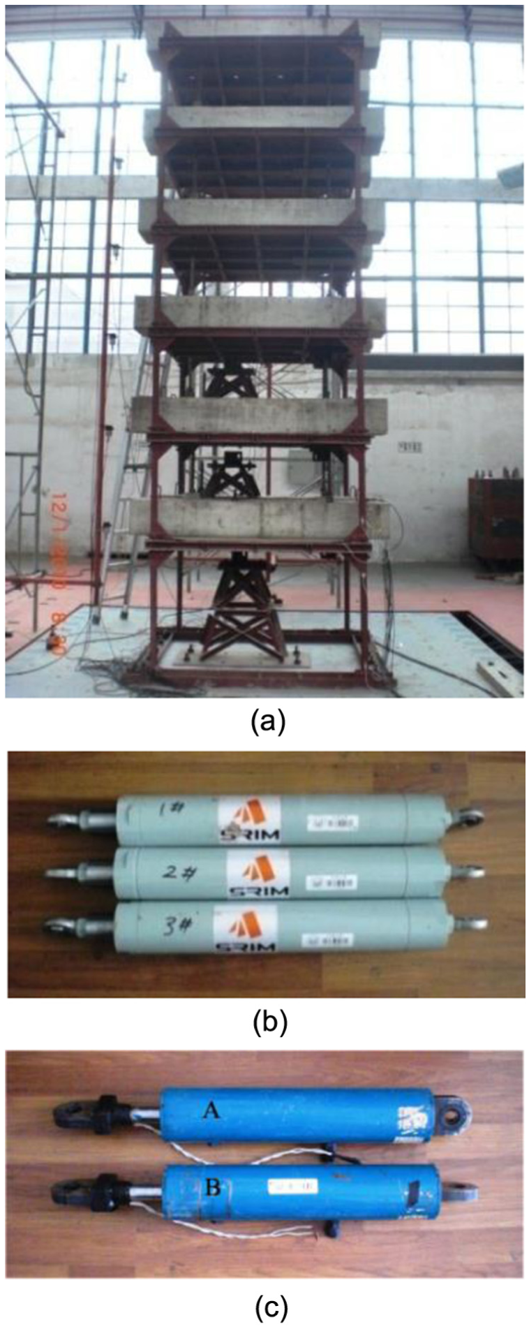
Photographs of tested structure and control devices: (a) tested structure, (b) three viscous dampers, and (c) two MR dampers.

Three viscous dampers and two magnetorheological (MR) dampers (marked as MRD-A and MRD-B, respectively) are employed as control devices in this experiment, as shown in Figure 2(b) and (c), respectively. These viscous dampers are designed as the same specifications, which exhibit a maximum force output of 10 kN, a stroke of ± 50 mm, and a length of 670 mm in their equilibrium position. Similarly, the two MR dampers have the same design parameters. Forces of up to 10 kN can be generated by the MR damper. It is of 725 mm long in its extended position, and the main cylinder is of 100 mm in diameter. The MR damper has a ± 55 mm stroke and its input current is in the range of 0–2 A.

In the stochastic seismic control experiments, the data are recorded by an automatic data acquisition system. An accelerometer, as well as a displacement transducer, is employed to measure the motion of the shaking table. Simultaneously, six accelerometers and six displacement transducers are mounted to measure the dynamic responses of each floor in the direction of seismic excitation. Moreover, three accelerometers and three displacement transducers are installed to measure the dynamic responses perpendicular to the direction of table motion.

Experimental program

In the stochastic control experiments, the time histories of representative ground accelerations previously generated are used as the one-dimensional (1D) input of shaking table. Since the tested structure is a scaled model, these ground accelerations need to be reproduced referring to the time scale factor, that is, the model-to-prototype ratio of time. Furthermore, it should be pointed out that the intensities of the representative ground accelerations should not be very high, especially in the uncontrolled cases so that the mechanical parameters of the structural model remain unchanged. The purpose of such design is to expose the influence of the randomness involved in seismic excitations by excluding other possible complex influential factors. Besides, dynamic responses of the tested model should not be too small to gain an obvious reduction of structural vibrations in case of control with dampers. As such, tradeoffs have to be achieved and consequently the peak accelerations of the input ground motions are fixed.

There are totally 363 cases as shown in Table 1. In the uncontrolled cases (Case Nos 1, 122, and 363), the ground acceleration W000 is considered as the seismic input, and the experimentally measured frequency response functions (FRFs) are used for the parameter identification of the tested structure. In the passive control-I cases (Case Nos 2 through 121), the three viscous dampers, as shown in Figure 2(b), are mounted on the bottom three floors while the two MR dampers, as shown in Figure 2(c), are installed as the control devices in the passive control-II cases (Case Nos 123 through 242). In detail, the MRD-A is placed between the ground and first floors, and the MRD-B is placed between the second and third floors of the model structure. Besides, the currents applied to the two MR dampers are held fixed at 1.5 A in the passive control-II cases. Among the uncontrolled cases (Case Nos 243 through 362), the steel structural model without dampers is tested. Comparing the dynamic responses of the model in the corresponding cases (with and without dampers under the same seismic input), the control effectiveness of the dampers can be investigated (Li et al., 2012b; Mei et al., 2013; Peng et al., 2014b).

Table 1.

Cases of experimental program.

Case number	Seismic input	Amplitude (m/s²)	Remark
1	W000	1.00	Without control
2–121	W001–W120	Min.: 0.39; Max.: 2.30; Mean: 1.09; SD: 0.28	Passive control: I (three viscous dampers installed)
122	W000	1.00	Without control
123–242	W001–W120	Min.: 0.78; Max.: 4.61; Mean: 2.18; SD: 0.56	Passive control: II (two MR dampers installed)
243–362	W001–W120	Min.: 0.39; Max.: 2.30; Mean: 1.09; SD: 0.28	Without control
363	W000	1.00	Without control

MR dampers: magnetorheological dampers; Min.: minimum; Max.: maximum; SD: standard deviation.

Identification of structural parameters

According to the FRFs integrated from the data measured in the uncontrolled cases (Case Nos 1, 122, and 363), dynamic characteristics as well as physical parameters of the tested structure without control can be identified.

The first six natural frequencies of the uncontrolled structure vary, respectively, from 1.476, 4.642, 8.419, 12.534, 16.835, 20.315 Hz (Case 1 in Table 1) to 1.460, 4.624, 8.365, 12.452, 16.803, 20.277 Hz (Case 122 in Table 1), and then to 1.453, 4.605, 8.338, 12.385, 16.745, 20.184 Hz (Case 363 in Table 1). It is seen that the first three natural frequencies only decreased by about 1.6%, 0.8%, and 1.0%, respectively, throughout the cases of the shaking table tests. Moreover, the first three mode shapes of the tested structure without dampers are pictured in Figure 3. It is clear that the first three modes remain almost unchanged. As such, it has reason to believe that the tested structure itself still remains within the range of linear elastic state in the whole experiment. Besides, it is measured that there is almost no structural motion perpendicular to the direction of table movement.

Figure 3.

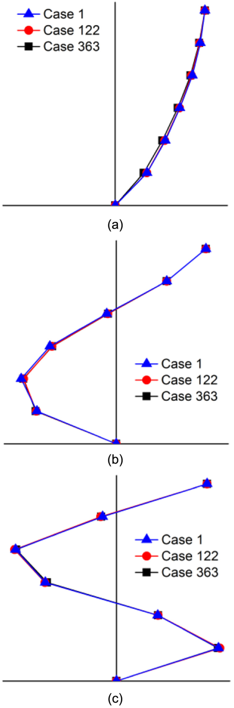
The first three mode shapes of the tested structure without control: (a) mode 1, (b) mode 2, and (c) mode 3.

Note that the tested structure itself is symmetrical and 1D ground motions are adopted as the input of shaking table, so it is needed to only pay attention to the translational characteristics of the model structure in the direction of seismic excitation. In addition, the mass of each story of the tested structure is mainly concentrated on the floor. Thus, the number of degrees of freedom (DOFs) of the model structure without dampers is reduced to 6, namely, 1 DOF for each story. The physical parameters, say the mass, stiffness, and damping matrices of the 6-DOF model can be identified as follows (Mei et al., 2012). The mass matrix of the 6-DOF model is determined by the mass of the model structure itself and the additional artificial quality. The stiffness matrix is calculated according to the first six natural frequencies and corresponding mode shapes, which can be identified from the experimentally measured FRFs. In addition, the damping ratios of the first two modes can be estimated by the method of half power points and thus the damping matrix is obtained according to the Rayleigh damping scheme. In order to verify the correctness of the identified 6-DOF model, the results of the shaking table test (Case No. 243) are compared with those of the numerical simulation, as shown in Figure 4. It is seen that the experimental and numerical results are in good overall agreement, indicating that the 6-DOF model can maintain the important dynamics of the tested structure.

Figure 4.

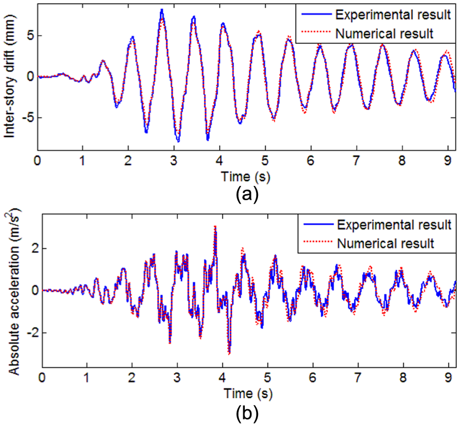
Comparisons of typical responses of the tested structure between experimental and numerical results: (a) inter-story drift of the first floor and (b) absolute acceleration of the top floor.

Verification of the PDEM based on results of stochastic seismic control experiments

In this section, the verification of the PDEM based on the results of stochastic seismic control experiments is carried out. In detail, experimentally measured typical responses (inter-story drift of the first floor and absolute acceleration of the top floor, similarly hereinafter) of the tested structure without dampers subjected to random seismic excitations (Case Nos 243 through 362) are analyzed by sample statistics and the PDEM, respectively. Then, analytical results based on the two different methods are compared in order to investigate the accuracy of the PDEM.

Comparisons of means and standard deviations

The means and standard deviations of structural responses, say, the first floor inter-story drift, the top floor absolute acceleration, and the top floor displacement (relative to the shaking table), evaluated through the PDEM are depicted in Figure 5, comparing with the results by sample statistics. On the whole, perfect accordance between the PDEM and sample statistics is seen, which demonstrates that the PDEM is of high accuracy.

Figure 5.

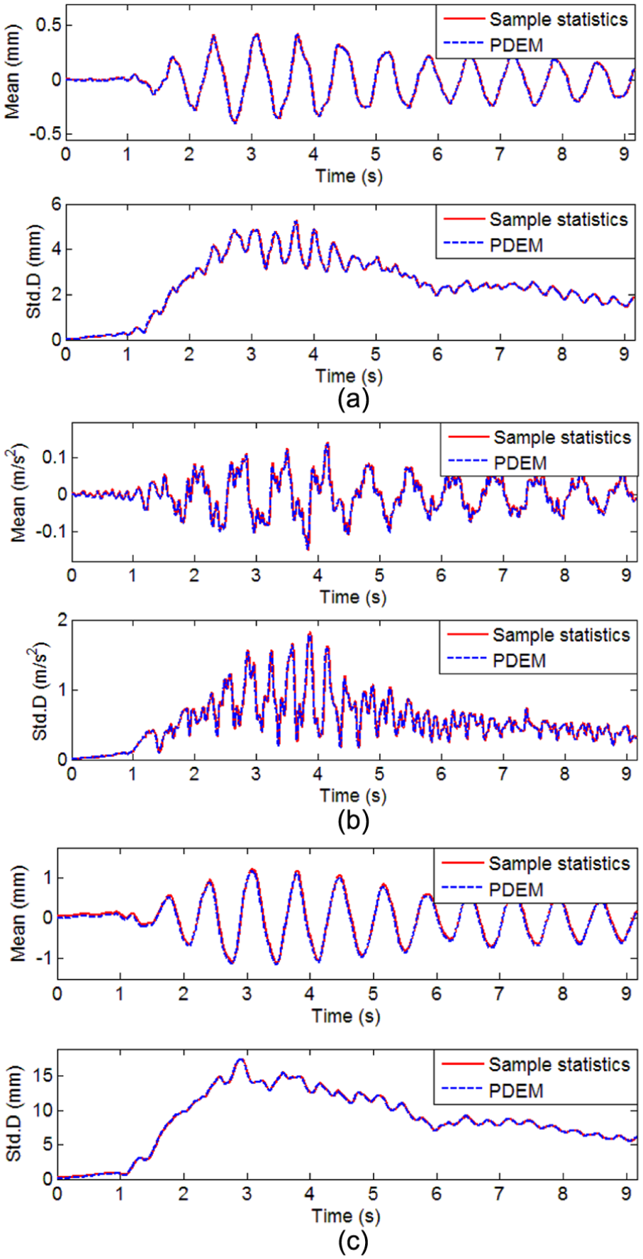
Comparisons of means and standard deviations of structural responses between sample statistics and PDEM: (a) inter-story drift of the first floor, (b) absolute acceleration of the top floor, and (c) top floor displacement.

To check the error more clearly, define the two-norm relative error

e_{‖ x ‖} = \frac{‖ \hat{x} (t) - x (t) ‖}{‖ x (t) ‖} \times 100 %

(9)

where $‖ \cdot ‖ denotes$ the two-norm $‖ x (t) ‖ = \sqrt{\sum_{j = 1}^{N} x^{2} (t_{j})}$ , in which N is number of the time step. Because the real exact solution $x (t)$ is unknown, the result obtained by sample statistics is adopted as the exact solution here. In Figure 5(a), the two-norm relative errors of the mean and standard deviation are 9.4% and 2.1%, respectively, both less than 10%. The two-norm relative errors of the mean and standard deviation in Figure 5(b) are 21.4% and 9.5%, respectively. In Figure 5(c), the two-norm relative errors are 12.6% and 1.9%, respectively. As such, it is creditable that the accuracy of the PDEM is fairly high in terms of the first- and second-order statistics.

Comparisons of PDFs and cumulated distribution functions

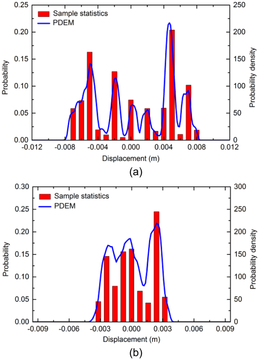
As mentioned in section “Introduction,” the instantaneous PDF and its evolution of stochastic responses are available through the PDEM. As a matter of fact, it is the PDF itself rather than the first- and second-order statistics that is evaluated in the analysis. The mean and standard deviation are just by-products. Shown in Figures 6 and 8 are the PDFs as well as the statistical histograms of typical responses of the tested structure at certain time instants, say, 3.0 and 8.0 s. The comparisons of cumulated distribution functions (CDFs) at two instants of time between the PDEM and sample statistics are pictured in Figures 7 and 9. The figures just referred to show that the analytical results by the PDEM accord well with the counterparts by sample statistics.

Figure 6.

Comparisons of PDFs of inter-story drift of the first floor at two instants of time between sample statistics and PDEM: (a) 3 s and (b) 8 s.

Figure 7.

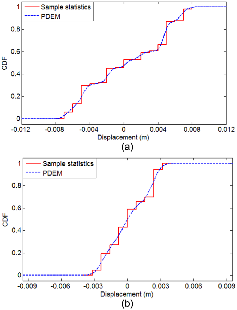
Comparisons of CDFs of inter-story drift of the first floor at two instants of time between sample statistics and PDEM: (a) 3 s and (b) 8 s.

In Figures 6 and 8, it is clearly seen that the PDFs are very consistent with the corresponding histograms in the sense of probability distributions. For instance, the distribution width of the PDF is almost the same as that of the histogram obtained by sample statistics. Furthermore, it is found that the PDF can capture the detailed characteristics of the probability distribution shown in the histogram, such as the distributions of peaks and valleys. In order to quantitatively compare the probability distributions obtained by sample statistics and the PDEM, relative entropies of corresponding distributions are calculated. The relative entropy of probability distributions P to Q can be expressed as D(P:Q) and can be defined as follows (Zhang et al., 2017)

D (P : Q) = \sum_{i} P_{i} \ln \frac{P_{i}}{Q_{i}}

(10)

Figure 8.

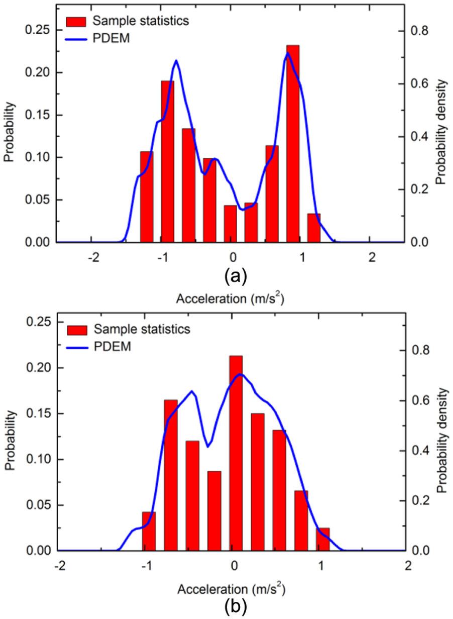
Comparisons of PDFs of absolute acceleration of the top floor at two instants of time between sample statistics and PDEM: (a) 3 s and (b) 8 s.

In this article, the probability distribution shown in the histogram is considered as the distribution P in equation (10), and the PDFs obtained by the PDEM should be changed to discrete probability distributions before calculating relative entropies. The relative entropies in Figure 6(a) and (b) are 0.128 and 0.110, respectively, and those in Figure 8(a) and (b) are 0.084 and 0.073, respectively. It is seen that the mean value of these relative entropies is less than 0.100.

As is well known, statistical histograms are somewhat sensitive to the size of statistical ranges, but statistical distribution functions are relatively robust. Thus, probability distribution functions are also given here, as shown in Figures 7 and 9. From the two figures, perfect agreement between the PDEM and sample statistics is also seen. It is obvious that the CDF by the PDEM can grasp the convexity and concavity of the corresponding statistical distribution function by sample statistics. In summary, it can be concluded that the PDEM is able to precisely capture the probability distributions of responses of stochastic dynamical systems.

Figure 9.

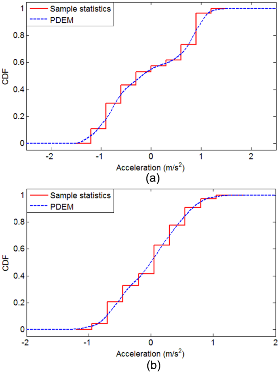
Comparisons of CDFs of absolute acceleration of the top floor at two instants of time between sample statistics and PDEM: (a) 3 s and (b) 8 s.

Evolution of PDF against time

As shown in Figures 6 and 8, the typical instantaneous PDFs at different instants of time are obviously not the same. It is true that the PDFs evolve greatly against time. Depicted in Figure 10 are continuous evolution processes of the PDF of inter-story drift of the first floor, including the PDF surface and the corresponding contour.

Figure 10.

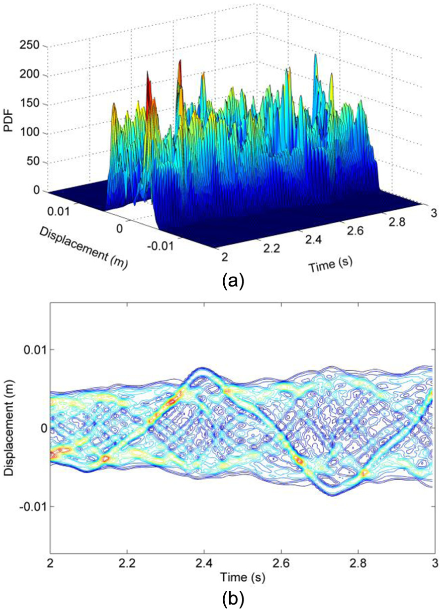
Evolution of PDF of inter-story drift of the first floor against time: (a) PDF surface and (b) contour to the PDF surface.

It is seen from Figure 10(a) that the PDF evolution surface is just like a mountain wriggling and stretching to the distance, usually with two or more ridges. The sections of the “mountain” are PDFs of inter-story drift of the first floor at certain instants of time, two of which are illustrated in Figure 6. The contour of the PDF surface, shown in Figure 10(b), seems like the water flowing in a river. However, the flow in the “river” is not stationary and there are many whirlpools. A whirlpool in the contour is related to a peak or valley of the “mountain” in Figure 10(a). The whirlpool structure in the “river” means that the PDF of the response is very complex and varies with time considerably. In a word, the PDEM can grasp the evolution processes of PDFs of dynamic responses of structures in detail.

Validation of the PDEM by numerical simulations

In the preceding section, the accuracy of the PDEM is verified based on the results of stochastic seismic control experiments. In order to further validate the correctness as well as the reliability of the method, numerical simulations are presented in this section. Stochastic dynamic response analyses of the tested structure without control subjected to three different groups of representative ground accelerations are conducted, respectively, and the results are compared.

Statistical characteristics of representative ground accelerations

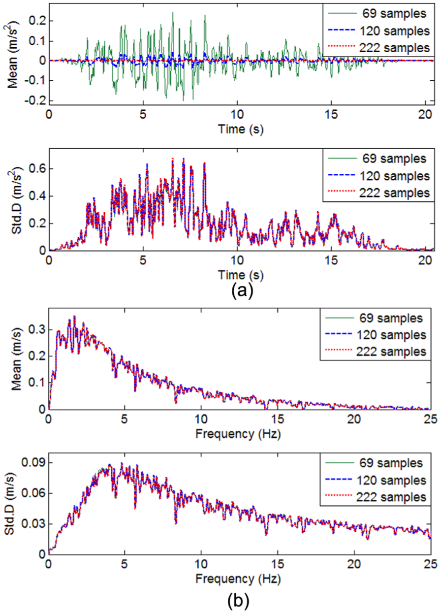
In addition to the ground motions (120 samples) obtained in section “Stochastic seismic control experiments,” other two sets of ground accelerations, containing 69 and 222 samples, respectively, are generated by employing the physical stochastic ground motion model (Li and Ai, 2006) and the strategy of selecting representative points via tangent spheres (Chen and Li, 2008). The mean and standard deviation of peak accelerations of the 69 samples are 1.08 and 0.28 m/s², respectively, and those of the 222 samples are 1.07 and 0.28 m/s², respectively. It is seen that the means and standard deviations of peak accelerations of the three different groups of samples are almost the same, respectively.

With the PDEM, the means and standard deviations of ground accelerations and Fourier amplitude spectra of different groups of samples are obtained, and the results are compared, respectively, as pictured in Figure 11. It is clear from Figure 11(a) that there are obvious differences among the mean processes of ground accelerations. As a matter of fact, the ground motions generated by the physical stochastic ground motion model is zero mean, especially when the number of representative samples is relatively large. Moreover, it is found from Figure 11 that the standard deviations of ground accelerations are very consistent, and so are the means and standard deviations of Fourier amplitude spectra, indicating that the second-order statistical characteristics of the three sets of ground motions are highly similar.

Figure 11.

Comparisons of means and standard deviations of ground accelerations and Fourier amplitude spectra: (a) ground accelerations and (b) Fourier amplitude spectra.

Statistical values of peak and root mean square responses

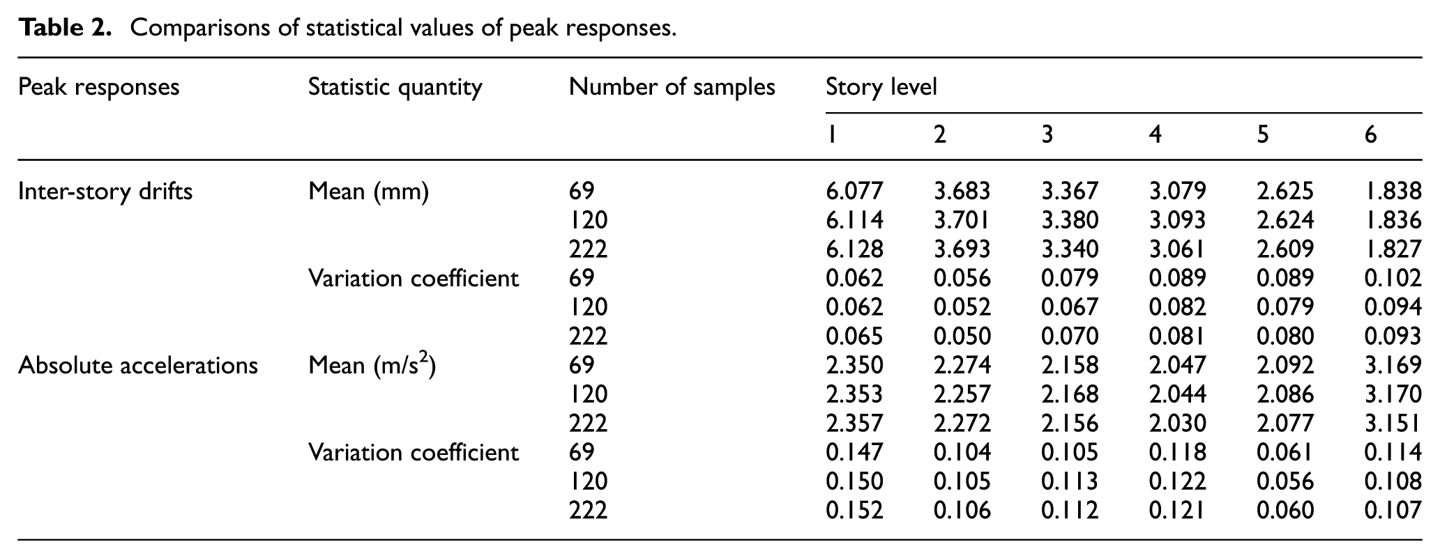
Dynamic responses of the tested structure without dampers, namely the identified 6-DOF model, subjected to the three groups of ground motions generated above are analyzed by programming based on MATLAB software. It should be noted that the physical parameters of the 6-DOF model have been obtained in section “Stochastic seismic control experiments,” and its correctness has been proved by comparing the experimental and numerical results (see Figure 4). Statistical values of the peak and root mean square (RMS) responses are given in Tables 2 and 3, respectively. It is seen that the corresponding statistical values, both means and variation coefficients, are close to each other. In Table 2, the relative errors of means of the peak responses are mostly no more than 1.0% and those of variation coefficients are usually less than 10.0%. The relative errors of means and variation coefficients of the RMS responses in Table 3 generally do not exceed 0.1% and 4.0%, respectively. Therefore, it can be concluded that relatively small representative samples are able to accommodate a comparatively accurate result of the first- and second-order statistical properties of peak and RMS responses of structures in the PDEM.

Table 2.

Comparisons of statistical values of peak responses.

Peak responses	Statistic quantity	Number of samples	Story level
			1	2	3	4	5	6
Inter-story drifts	Mean (mm)	69	6.077	3.683	3.367	3.079	2.625	1.838
		120	6.114	3.701	3.380	3.093	2.624	1.836
		222	6.128	3.693	3.340	3.061	2.609	1.827
	Variation coefficient	69	0.062	0.056	0.079	0.089	0.089	0.102
		120	0.062	0.052	0.067	0.082	0.079	0.094
		222	0.065	0.050	0.070	0.081	0.080	0.093
Absolute accelerations	Mean (m/s²)	69	2.350	2.274	2.158	2.047	2.092	3.169
		120	2.353	2.257	2.168	2.044	2.086	3.170
		222	2.357	2.272	2.156	2.030	2.077	3.151
	Variation coefficient	69	0.147	0.104	0.105	0.118	0.061	0.114
		120	0.150	0.105	0.113	0.122	0.056	0.108
		222	0.152	0.106	0.112	0.121	0.060	0.107

Table 3.

Comparisons of statistical values of RMS responses.

RMS responses	Statistic quantity	Number of samples	Story level
			1	2	3	4	5	6
Inter-story drifts	Mean (mm)	69	2.303	1.482	1.257	1.063	0.800	0.517
		120	2.303	1.482	1.256	1.063	0.801	0.517
		222	2.303	1.481	1.256	1.063	0.800	0.517
	Variation coefficient	69	0.052	0.055	0.053	0.050	0.043	0.034
		120	0.052	0.055	0.052	0.049	0.043	0.033
		222	0.051	0.054	0.051	0.048	0.042	0.033
Absolute accelerations	Mean (m/s²)	69	0.553	0.567	0.585	0.609	0.635	0.798
		120	0.553	0.568	0.585	0.609	0.636	0.798
		222	0.554	0.568	0.585	0.608	0.635	0.798
	Variation coefficient	69	0.136	0.078	0.054	0.058	0.028	0.041
		120	0.136	0.079	0.053	0.057	0.028	0.041
		222	0.134	0.077	0.053	0.057	0.027	0.040

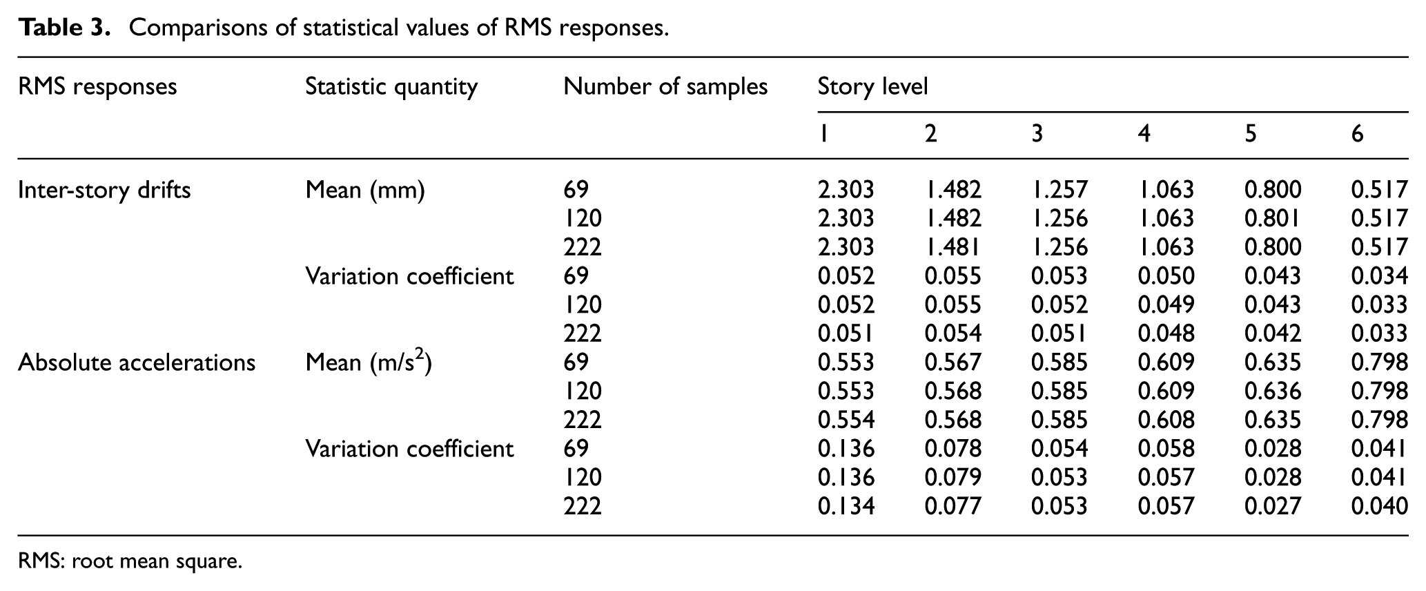
RMS: root mean square.

Means and standard deviations of typical responses

Stochastic dynamic response analyses of the tested structure without control subjected to the three different groups of representative ground motions are conducted using the PDEM. The means and standard deviations of typical responses are presented in Figure 12. The comparisons in this figure show that the standard deviations of typical responses are very close. The maximum two-norm relative errors are 7.1% and 6.9% in Figure 12(a) and (b), respectively. At the same time, it is easily seen from Figure 12 that the means of typical responses are close to zero with the increase in the number of representative ground motions. As a matter of fact, the ground motions generated by the physical stochastic ground motion model is zero mean, especially when the number of representative samples is relatively large.

Figure 12.

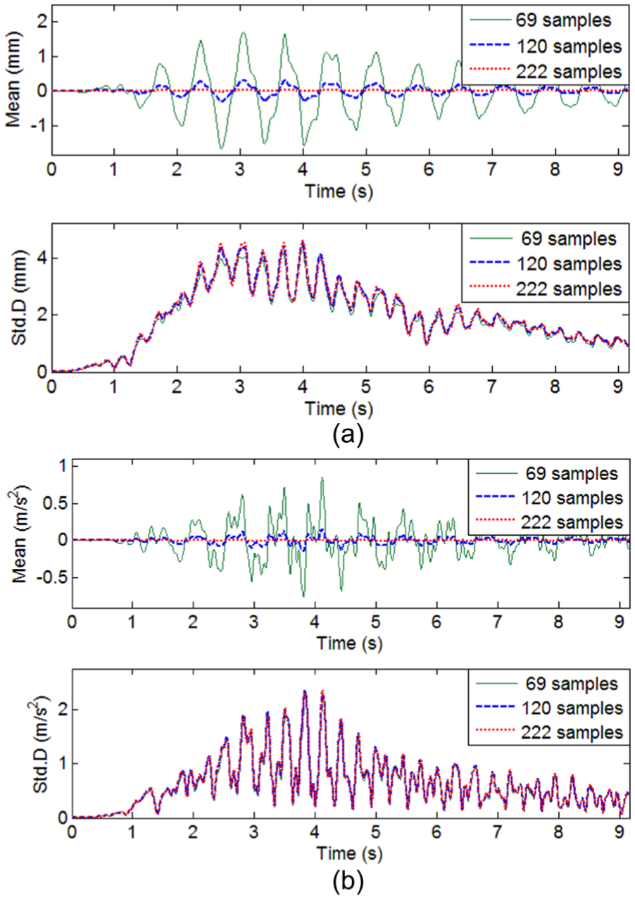
Comparisons of means and standard deviations of typical responses: (a) inter-story drift of the first floor and (b) absolute acceleration of the top floor.

PDFs of typical responses

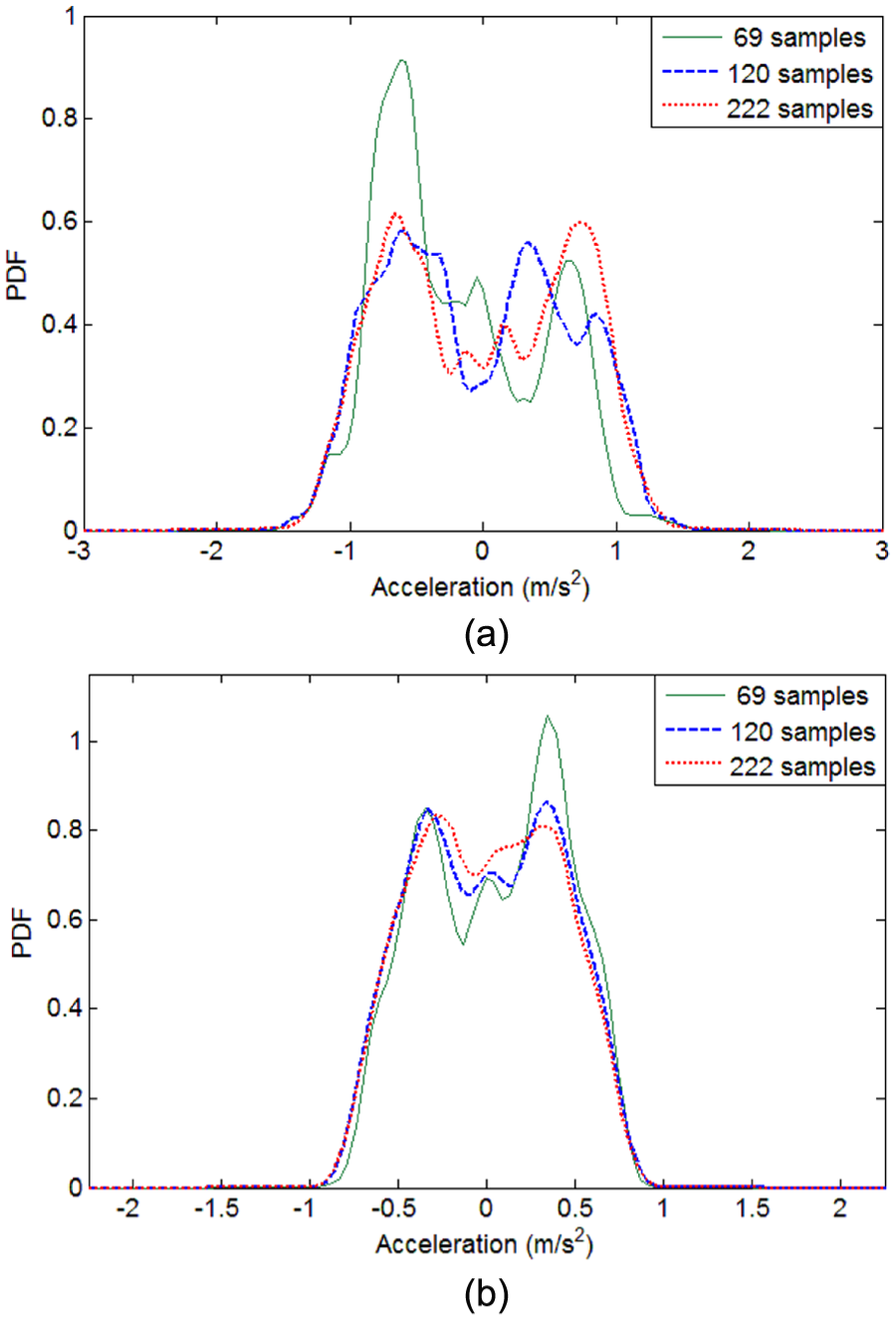
Besides the means and standard deviations, instantaneous PDFs of typical responses of the tested structure are simultaneously available through the PDEM, as pointed out in the foregoing section. Figures 13 and 14, respectively, show the comparisons of PDFs of inter-story drift of the first floor and absolute acceleration of the top floor at two instants of time, say, 3.0 and 8.0 s. It is found in the first place that the PDFs of typical responses at a given instant of time have almost the same distribution width. Furthermore, the overall trends of the PDFs are almost unanimous. On the other hand, it is also seen that there are certain differences among the PDFs, for instance, the distributions of peaks and valleys in the curves.

Figure 13.

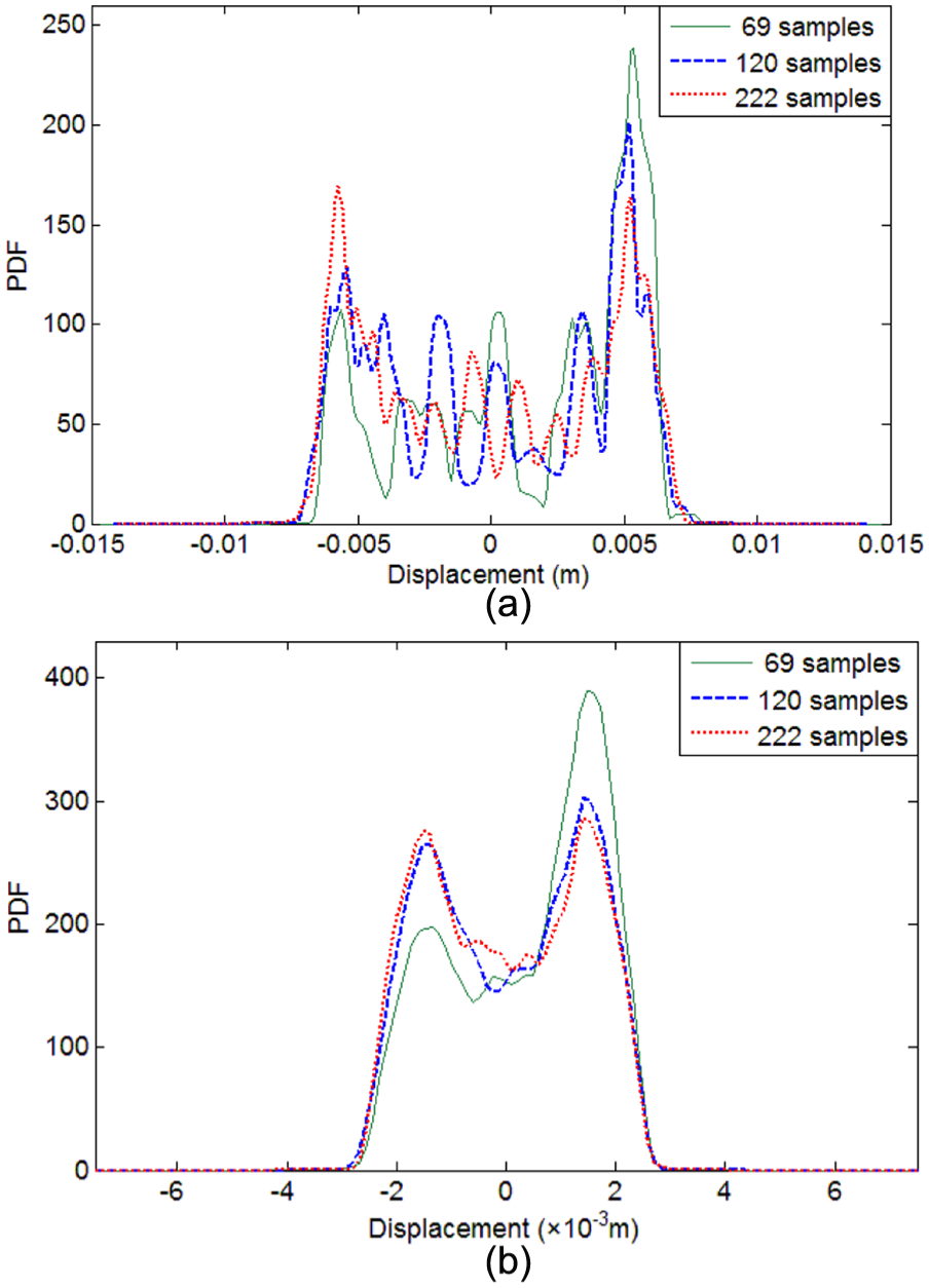
Comparisons of PDFs of inter-story drift of the first floor at two instants of time: (a) 3 s and (b) 8 s.

Figure 14.

Comparisons of PDFs of absolute acceleration of the top floor at two instants of time: (a) 3 s and (b) 8 s.

Contours of PDF surfaces of typical responses

Plotted in Figure 15 are the contours of PDF surfaces of absolute acceleration of the top floor of the tested structure subjected to three different sets of ground motions. It is noted that there are no significant differences among the three contours on the whole. The contours presented here show a great degree of similarity in the distribution width at each instant of time as well as the overall distribution pattern. That is to say, a relatively small amount of representative samples is able to lead to a comparatively high accuracy analysis of stochastic dynamical systems, indicating the efficiency as well as the accuracy of the PDEM. Besides, it is also found in Figure 15 that the detailed configuration structures of the three contours are distinct to some extent because of the different numbers of representative ground motions.

Figure 15.

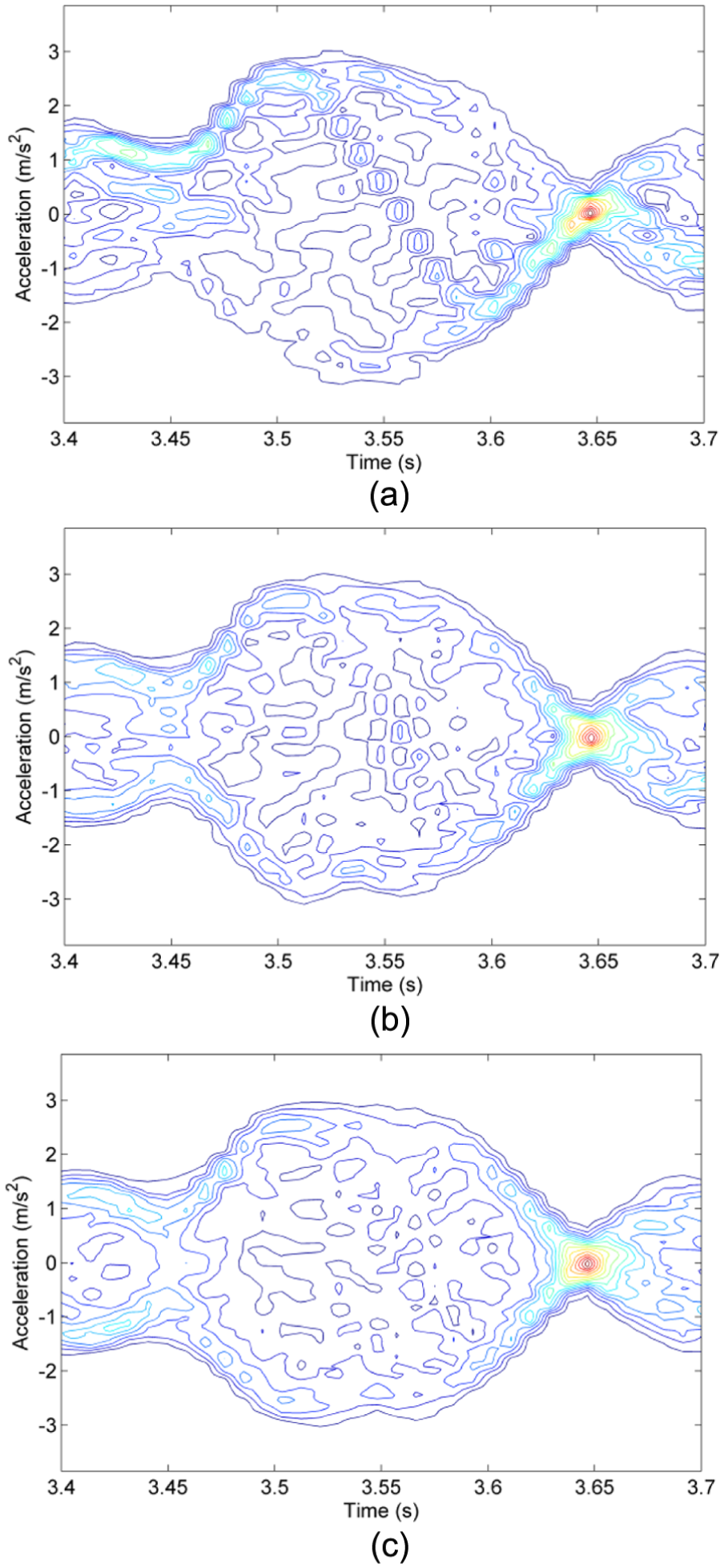
Comparison of contours of PDF surfaces of absolute acceleration of the top floor: (a) 69 samples, (b) 120 samples, and (c) 222 samples.

Concluding remarks

In this article, the accuracy and efficiency of the PDEM are investigated based on the results of shaking table tests of a randomly base-driven structure, and the correctness and reliability of the PDEM are also examined using the results of stochastic response analyses of the tested structure model subjected to three different sets of representative ground motions. The following conclusions could be drawn:

The two-norm relative errors of means and standard deviations of structural responses analyzed by sample statistics and the PDEM are usually no more than 10%. So it is creditable that the accuracy of the PDEM is fairly high in terms of the first- and second-order statistics.

The mean value of relative entropies of probability distributions of typical responses at two instants of time is less than 0.100. Therefore, it can be concluded that the PDEM is able to precisely capture the probability distributions of responses of stochastic dynamical systems.

The relative errors of means and variation coefficients of peak and RMS responses of the model structure subjected to three different groups of ground motions generally do not exceed 1.0% and 10.0%, respectively, and the maximum two-norm relative errors of standard deviations of typical responses are only about 7.0%. It can thus be seen that relatively small representative samples are able to accommodate a comparatively accurate result of the first- and second-order statistical properties in the PDEM.

Instantaneous PDFs and their evolutions of typical responses of the model structure subjected to three different sets of ground motions show close similarities in distribution width as well as overall distribution pattern, respectively, indicating the efficiency and accuracy of the PDEM. Moreover, it is found that the number of representative samples has a certain influence on the analytical results of the PDEM, especially when the PDF and its evolution of responses are concerned.

Footnotes

Declaration of Conflicting Interest

The author(s) declared no potential conflicts of interest with respect to the research, authorship, and/or publication of this article.

Funding

The author(s) disclosed receipt of the following financial support for the research, authorship, and/or publication of this article: This work was supported by the National Natural Science Foundation of China (Grant Nos. 51578254 and 51608212) and the Natural Science Foundation of Fujian Province, China (Grant No. 2015J01211) are highly appreciated.

References

Anderson

(1995) Computational Fluid Dynamics. New York: McGraw-Hill.

Chen

(2007) The extreme value distribution and dynamic reliability analysis of nonlinear structures with uncertain parameters. Structural Safety 29(2): 77–93.

Chen

(2008) Strategy for selecting representative points via tangent spheres in the probability density evolution method. International Journal for Numerical Methods in Engineering 74(13): 1988–2014.

Chopra

(2011) Dynamics of Structures, Theory and Applications to Earthquake Engineering. 4th ed. Upper Saddle River, NJ: Prentice-Hall.

Clough

Penzien

(1993) Dynamics of Structures. 2nd ed.New York: McGraw-Hill.

Dowrick

(2003) Earthquake Risk Reduction. Chichester: John Wiley & Sons.

Ghanem

Spanos

(1991) Stochastic Finite Element: A Spectral Approach. Berlin: Springer.

Kozin

(1961) On the probability densities of the output of some random systems. Journal of Applied Mechanics 28(2): 161–164.

(1996) Stochastic Structural Systems: Analysis and Modeling. Beijing, China: Science Press (in Chinese).

10.

(2016) Probability density evolution method: background, significance and recent developments. Probabilistic Engineering Mechanics 44: 111–117.

11.

(2006) Study on random model of earthquake ground motion based on physical process. Earthquake Engineering and Engineering Vibration 26 (5): 21–26 (in Chinese).

12.

Chen

(2004) Probability density evolution method for dynamic response analysis of structures with uncertain parameters. Computational Mechanics 34(5): 400–409.

13.

Chen

(2005a) Dynamic response and reliability analysis of structures with uncertain parameters. International Journal for Numerical Methods in Engineering 62(2): 289–315.

14.

Chen

(2005b) Dynamic response and reliability analysis of non-linear stochastic structures. Probabilistic Engineering Mechanics 20(1): 33–44.

15.

Chen

(2006a) The probability density evolution method for dynamic response analysis of non-linear stochastic structures. International Journal for Numerical Methods in Engineering 65(6): 882–903.

16.

Chen

(2006b) The dimension-reduction strategy via mapping for probability density evolution analysis of nonlinear stochastic systems. Probabilistic Engineering Mechanics 21(4): 442–453.

17.

Chen

(2007) The number theoretical method in response analysis of nonlinear stochastic structures. Computational Mechanics 39(6): 693–708.

18.

Chen

(2008) The principle of preservation of probability and the generalized density evolution equation. Structural Safety 30(1): 65–77.

19.

Chen

(2009) Stochastic Dynamics of Structures. Singapore: John Wiley & Sons.

20.

Chen

Fan

(2007) The equivalent extreme-value event and evaluation of the structural system reliability. Structural Safety 29(2): 112–131.

21.

Chen

Sun

et al . (2012a) Advances of the probability density evolution method for nonlinear stochastic systems. Probabilistic Engineering Mechanics 28: 132–142.

22.

Mei

Chen

et al . (2012b) Experimental investigations of stochastic control of randomly base-excited structures. Advances in Structural Engineering 15(11): 1963–1975.

23.

Peng

Chen

(2010) A physical approach to structural stochastic optimal controls. Probabilistic Engineering Mechanics 25(1): 127–141.

24.

Lin

Zhang

(2004) Pseudo Excitation Method of Random Vibration. Beijing, China: Science Press (in Chinese).

25.

Lin

Cai

(1995) Probabilistic Structural Dynamics: Advanced Theory and Applications. New York: McGraw-Hill.

26.

Lutes

Sarkani

(2004) Random Vibrations: Analysis of Structural and Mechanical Systems. Amsterdam: Elsevier.

27.

Mei

Chen

(2012) Experimental design of structural vibration control subject to random earthquake ground motions. World Information on Earthquake Engineering 28(1): 157–163 (in Chinese).

28.

Mei

Peng

(2013) Experimental and analytical studies on stochastic seismic response control of structures with MR dampers. Earthquakes and Structures 5(4): 395–416.

29.

Peng

Chen

(2014a) Nonlinear response of structures subjected to stochastic excitations via probability density evolution method. Advances in Structural Engineering 17(6): 801–816.

30.

Peng

Mei

(2014b) Stochastic seismic response analysis and reliability assessment of passively damped structures. Journal of Vibration and Control 20(15): 2352–2365.

31.

Syski

(1967) Stochastic differential equations. In: Saaty

(ed.) Modern Non-linear Equations. New York: McGraw-Hill, pp. 346–456.

32.

Wang

(2011) Physical random function model of ground motions for engineering purpose. Science China: Technological Sciences 54(1): 175–182.

33.

(2016) Stochastic dynamic response and reliability assessment of controlled structures with fractional derivative model of viscoelastic dampers. Mechanical Systems and Signal Processing 72–73: 865–896.

34.

Zhang

Liu

et al . (2017) Constructing a measurement method of differences in group preferences based on relative entropy. Entropy 19(1): 24.

35.

Zhu

(2003) Nonlinear Stochastic Dynamics and Control in Hamiltonian Formulation. Beijing, China: Science Press (in Chinese).