Effects of free-stream turbulence on wind loads on a full-scale large cooling tower

Abstract

The high variability in turbulence is a significant feature of the realistic atmospheric boundary layer winds which might have strong effects on wind loads on structures submerged in atmospheric boundary layer. This article has been devoted to this matter of science which is of practical importance to wind-engineering design and research. First, the variation of the turbulence intensity of the atmospheric boundary layer flow has been studied using theoretical calculations and meteorological wind measurements. Second, the effects of free-stream turbulence on wind loads on circular cylindrical structures have been revealed at high Reynolds number and equivalent conditions based on field measurements and wind tunnel model tests for wind effects on a large cooling tower. Through these works, it is found that the turbulence intensity for the measured atmospheric boundary layer winds is highly variable due to the significant effect of the mean wind speed, which is not well represented by the traditional empirical formulae. Besides, the free-stream turbulence significantly influences the dynamic characteristics of wind effects on the cooling tower in most cases, and the wind effects for a flow field of high turbulence intensity are generally more unfavorable than those for a flow field of low turbulence intensity.

Keywords

atmospheric boundary layer flow cooling tower field measurement turbulence intensity wind effect

Model test results

Flows generated in atmospheric boundary layer (ABL) are usually turbulent, and a significant feature of the realistic ABL turbulence is that it is highly variable. According to Codes of Practice (e.g. DL/T 5339-2006:2006, 2006; GB 50009-2001:2002, 2002; GB/T 50102-2003:2003, 2003) and monographs (e.g. Holmes, 2001; Simiu and Scanlan, 1996), ABL flow fields can be simply divided into four types according to the roughness length of the ground surface. Empirical formulae of the mean wind velocity profile are given for each flow field type by Codes of Practice and monographs based on on-site observations, but the turbulence intensity profiles cannot be definitively described. This is because that the ground surface roughness length varies in an interval for each terrain type which causes uncertainties to the turbulence intensity (Holmes, 2001), and there might be other influences to the turbulence intensity which deserves further investigations. On the other hand, according to Niemann and Hölscher (1990), the three factors influencing the flow around a circular cylinder are the Reynolds number (Re), the surface roughness of the cylinder, and the turbulence intensity of the oncoming flow, so the attempts to reveal wind effects on circular cylinders submerged in ABL flow fields should take into account the realistic free-stream turbulence of the oncoming flow. Since the free-stream turbulence for ABL flow fields is highly variable, it is of practical significance to quantify the effects of free-stream turbulence on wind loads on circular cylindrical structures for either wind-engineering design or research.

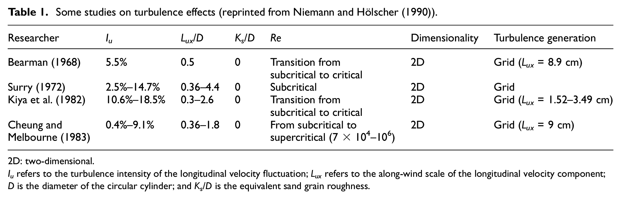
So far, some researches have been conducted in wind tunnels to quantify the effects of free-stream turbulence on the flow around a circular cylinder, whose main features are listed in Table 1. Reviewing these studies, some conclusions are drawn by Niemann and Hölscher (1990): (1) the effects of large-scale turbulence (integral length scale L_ux/D > 10) can be predicted by quasi-steady theory. Small-scale turbulence interacts with the boundary layer and the free shear layer. The scale itself does not seem to have an influence if L_ux/D < 1, whereas turbulence intensity does. (2) The transitional Re from subcritical to critical regime is shifted to lower values with increasing turbulence intensity due to earlier transition from laminar to turbulence flow. Some parameters are well correlated with the parameter Re^1.34I_u(d/L_ux)^0.2. (3) The separation is shifted downstream as turbulence intensity increases. The drag in the subcritical regime is then reduced. In the supercritical regime, the effect is opposite: base pressure and drag increase in spite of later separation. It is suggested that free-stream turbulence not only penetrates the boundary layer but also interacts with the free shear layer and the wake. (4) Strouhal number increases with the increase in turbulence intensity, simultaneously the spanwise correlation of vortices and root-mean-square lift are affected. Undoubtedly, the studies reviewed by Niemann and Hölscher (1990) are of high theoretical significance. However, it should be noted in Table 1 that most of those studies are conducted in wind tunnels with Re below transcritical regime, and the obtained results might hardly be applicable to the full-scale condition with high Re, since fluid flows around semi-aerodynamic bluff bodies largely depend on Re. To this end, it is of practical significance to conduct related researches at high Re employing effective experimental techniques. As it is extremely difficult to increase Re in wind tunnels by increasing model sizes (Dragoiescu et al., 2011; Matsuda et al., 2001) or pressurizing test channels (Achenbach, 1968; Roshko, 1961), the most practical approach to obtain results at high Re is the full-scale measurement.

Table 1.

Some studies on turbulence effects (reprinted from Niemann and Hölscher (1990)).

Researcher	I_u	L_ux/D	Re	Dimensionality	Turbulence generation
Bearman (1968)	5.5%	0.5	Transition from subcritical to critical	2D	Grid (L_ux = 8.9 cm)
Surry (1972)	2.5%–14.7%	0.36–4.4	Subcritical	2D	Grid
Kiya et al. (1982)	10.6%–18.5%	0.3–2.6	Transition from subcritical to critical	2D	Grid (L_ux = 1.52–3.49 cm)
Cheung and Melbourne (1983)	0.4%–9.1%	0.36–1.8	From subcritical to supercritical (7 × 10⁴–10⁶)	2D	Grid (L_ux = 9 cm)

2D: two-dimensional.

I_u refers to the turbulence intensity of the longitudinal velocity fluctuation; L_ux refers to the along-wind scale of the longitudinal velocity component; D is the diameter of the circular cylinder; and K_s/D is the equivalent sand grain roughness.

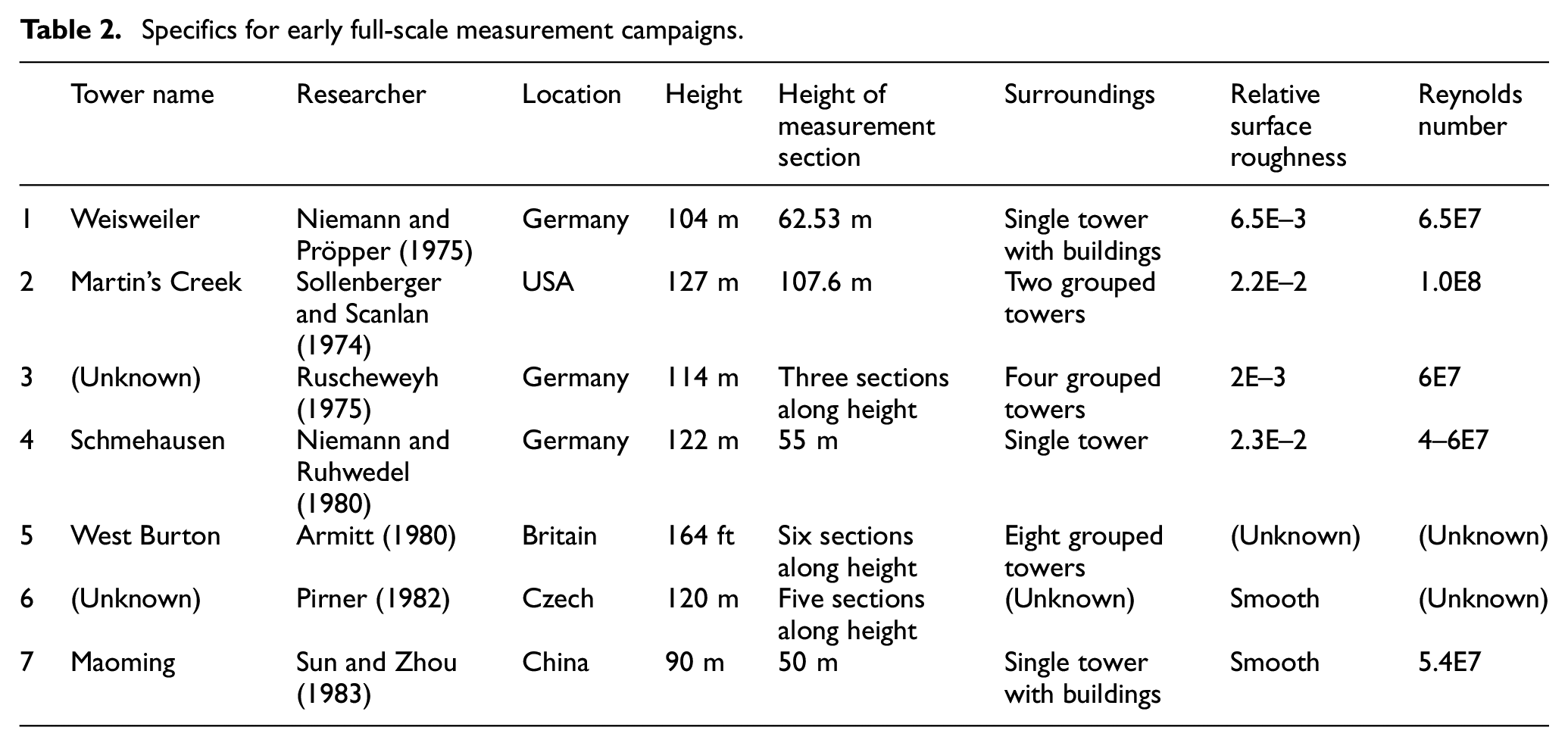
In history, many full-scale measurement campaigns for wind effects on cooling towers have been launched. The engineering backgrounds include 104-m Weisweiler cooling tower (Niemann, 1971; Niemann and Pröpper, 1975), 130-m Martin’s Creek cooling tower (Sollenberger and Scanlan, 1974), 122-m Schmehausen cooling tower (Niemann and Ruhwedel, 1980), and 90-m Maoming cooling tower (Sun and Zhou, 1983), whose specifics are listed in Table 2. The early field measurement campaigns listed in Table 2 are significant scientific endeavors. Unfortunately, most related researchers disregard the effects of free-stream turbulence on the measured wind loads in their studies. By reviewing literatures reporting results of these early full-scale measurement campaigns, it is found that only Niemann and Pröpper (1975) gave attention to the free-stream turbulence effects. They attributed the small fluctuating wind pressure coefficients measured on Weisweiler cooling tower to the low turbulence in the oncoming flow.

Table 2.

Specifics for early full-scale measurement campaigns.

	Tower name	Researcher	Location	Height	Height of measurement section	Surroundings	Relative surface roughness	Reynolds number
1	Weisweiler	Niemann and Pröpper (1975)	Germany	104 m	62.53 m	Single tower with buildings	6.5E–3	6.5E7
2	Martin’s Creek	Sollenberger and Scanlan (1974)	USA	127 m	107.6 m	Two grouped towers	2.2E–2	1.0E8
3	(Unknown)	Ruscheweyh (1975)	Germany	114 m	Three sections along height	Four grouped towers	2E–3	6E7
4	Schmehausen	Niemann and Ruhwedel (1980)	Germany	122 m	55 m	Single tower	2.3E–2	4–6E7
5	West Burton	Armitt (1980)	Britain	164 ft	Six sections along height	Eight grouped towers	(Unknown)	(Unknown)
6	(Unknown)	Pirner (1982)	Czech	120 m	Five sections along height	(Unknown)	Smooth	(Unknown)
7	Maoming	Sun and Zhou (1983)	China	90 m	50 m	Single tower with buildings	Smooth	5.4E7

In 2010, a new field measurement campaign for wind effects on Peng-cheng cooling tower located in Xu-zhou, China was launched by Tongji University. From 2011 to 2015, a total of 4000-h long strong wind velocity samples and wind pressure time-histories have been simultaneously measured on the location. Utilizing the available data, this article quantifies the effects of free-stream turbulence on wind loads on circular cylindrical structures at high Re. Furthermore, the results of full-scale measurements are validated by model tests carried out in a wind tunnel with an effective method to simulate high Re effects. With regard to the fact that most related studies are conducted in wind tunnels with inapplicable low Re and most researches based on early full-scale measurement campaigns disregard the effects of free-stream turbulence, this article explores an uncharted scientific territory.

Variability of the turbulence generated in ABL

Traditional empirical turbulence intensity profile envelopes

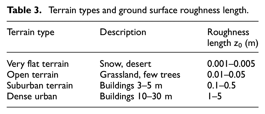
A 167-m high smooth-walled cooling tower was to be built in Peng-cheng electric power station, Xu-zhou, China. To its south, an adjacent cooling tower of the same size would be built too, and there was an industrial complex to its west (see Figure 1). To its north and east, there is no large interfering building, but a few mounds. According to the descriptions of terrain types given in Table 3 (Holmes, 2001), the flow field at Peng-cheng electric power station is open terrain type, for which the ground surface roughness length z₀ is in between 0.01 and 0.05 m.

Figure 1.

Site plan of Peng-cheng electric power station (m).

Table 3.

Terrain types and ground surface roughness length.

Terrain type	Description	Roughness length z₀ (m)
Very flat terrain	Snow, desert	0.001–0.005
Open terrain	Grassland, few trees	0.01–0.05
Suburban terrain	Buildings 3–5 m	0.1–0.5
Dense urban	Buildings 10–30 m	1–5

According to Simiu and Scanlan (1996) and Holmes (2001), the following equation exists

U (z) = \frac{1}{k} u_{*} \ln \frac{z}{z_{0}}

(1)

where z is the height above the surface, u_* is the friction velocity, U(z) is the mean wind speed at z height, and k = 0.4. Using equation (1), the friction velocity u_* is calculated for the site of Peng-cheng electric power station assuming that the mean wind velocity is the basic design value of 50-year return according to GB 50009-2001:2002 (2002), which is 1.35–1.76 m/s.

According to Simiu and Scanlan (1996), the longitudinal turbulence intensity at z height I(z) is defined as

I (z) = \frac{σ_{u}}{U (z)}

(2)

where σ_u is the root mean square value of the longitudinal velocity fluctuation u, which does not vary with height based on the common assumption, and can be written as

σ_{u}^{2} = β u_{*}^{2}

(3)

where β does not vary with height and only changes according to the variation of the ground surface roughness length. Thus, it can be found by substituting equations (1) and (3) into equation (2) that according to the empirical formulae, the longitudinal turbulence intensity at z height, I(z) is unrelated to the mean wind speed at z height U(z), but it depends on the ground surface roughness length z₀ and elevation z.

Values of β suggested by Bietry et al. (1978) for structural design purposes are based on a large number of measurements, which are listed in Table 4. Using the first-order exponential decay equation to fit data presented in Table 4, the following relation between z₀ and β can be obtained

β = 2.27 \exp (- \frac{z_{0}}{0.68}) + 4.05

(4)

Table 4.

Value of β corresponding to various ground surface roughness lengths.

z₀ (m)	0.005	0.07	0.3	1	2.5
β	6.5	6	5.25	4.85	4

According to equation (4), the value β for open terrain type is 6.29–6.16. Then, according to equation (3), σ_u for open terrain type is 3.39–4.37 m/s. Thus, the empirical turbulence intensity profile for the site of Peng-cheng electric power station can be calculated using equation (2) assuming that the mean wind velocity is the basic design value of 50-year return according to GB 50009-2001:2002 (2002). As shown in Figure 2, the empirical turbulence intensity profile varies in the interval between the lower and upper envelopes due to the uncertainty of the ground surface roughness length.

Figure 2.

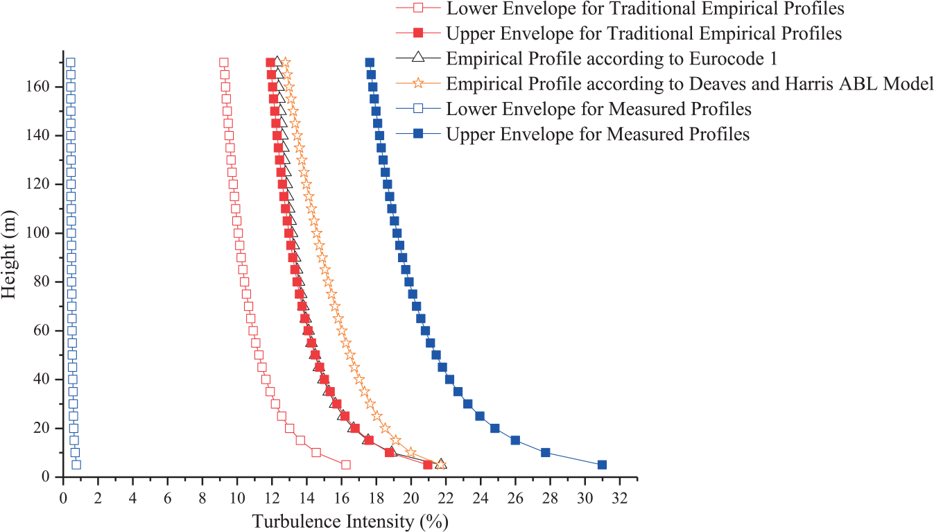
Measured and empirical turbulence intensity profiles.

Empirical turbulence intensity profile according to Eurocode 1

Same as the traditional empirical mean wind velocity profile, the mean wind velocity profile presented in EN 1991-1-4: 2004 (2004) also follows a logarithmical curve. However, the mathematical expressions for wind velocities in Eurocode 1 are different from the traditional empirical formulae, which definitively describe the wind velocities for each terrain type. According to Eurocode 1, the mean wind velocity profile is defined as

U (z) = 0.19 {(\frac{z_{0}}{z_{0, ∥}})}^{0.07} \ln (\frac{z}{z_{0}}) V_{b}

(5)

where $V_{b}$ is the basic wind velocity defined at 10 m above ground of terrain category II as a function of wind direction and time of year, and Z_0,II = 0.05 m is the aerodynamic ground surface roughness length for terrain category II. The turbulence intensity profile is given in equation (6) given that the effects of orography are neglected and the turbulence factor is the recommended value 1.0

I (z) = \frac{1}{\ln (z / z_{0})}

(6)

According to EN 1991-1-4: 2004 (2004), the terrain at the engineering site of Peng-cheng electric power station belongs to category II. Thus, the turbulence intensity profile for Peng-cheng electric power station can be calculated using equation (6) with z₀ = 0.05 m. As can be seen in Figure 2, the empirical turbulence intensity profile according to Eurocode 1 overlaps the upper envelope of traditional empirical profiles.

Empirical turbulence intensity profile according to Deaves and Harris ABL model

The wind analysis in practical projects generally uses the Deaves and Harris log-law ABL wind model (Cook, 1997) as defined in ESDU 01008:2005 (2005). Such a practice is supported by Cook (1997), Drew et al. (2013), Gualtieri (2017), and Tieleman (2008). The Deaves and Harris ABL model can take account of the variation of the upwind terrain on each wind sector. Therefore, it is believed that the wind analysis using the Deaves and Harris ABL model is more reasonable rather than those presented by Simiu and Scanlan (1996) and Holmes (2001) in the practical project. The primary equations for Deaves and Harris ABL model are as follows.

The gradient height is

h = \frac{u_{*}}{6 f}

(7)

where the Coriolis parameter

f = 2 Ω \sin ϕ

(8)

with $Ω$ the rate of rotation of the earth and $ϕ$ the latitude. According to Richards and Norris (2015), Ω = 72.9 × 10^–6 rad/s, and φ = 45° for countries in Asia. Thus, f = 1.03 × 10^–4 rad/s

The velocity profile is

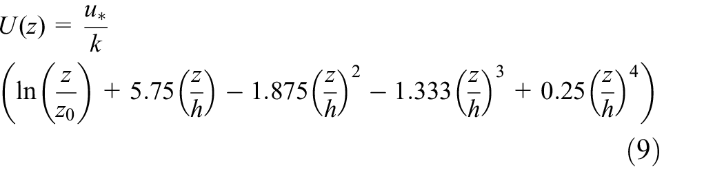
\begin{matrix} U (z) = \frac{u_{*}}{k} \\ (\ln (\frac{z}{z_{0}}) + 5.75 (\frac{z}{h}) - 1.875 {(\frac{z}{h})}^{2} - 1.333 {(\frac{z}{h})}^{3} + 0.25 {(\frac{z}{h})}^{4}) \end{matrix}

(9)

The standard deviation of the along-wind component of the wind velocity is given by

\frac{σ_{u} (z)}{u_{*}} = 2.63 η [0.538 + 0.09 \ln (z / z_{0})]^{m}

(10)

where $η = 1 - z / h$ and $m = η^{16}$ . Using equations (7) to (10), the empirical turbulence intensity profile according to Deaves and Harris ABL model is calculated with z₀ = 0.05 m. As shown in Figure 2, the empirical turbulence intensity profile according to Deaves and Harris ABL model is slightly greater than the upper envelope of traditional empirical profiles.

Measured turbulence intensity profile envelopes

Before the construction of the two-grouped cooling towers, a two-dimensional (2D) propeller anemometer, a three-dimensional (3D) ultrasonic anemometer, and a vane are arranged together at the engineering site at 20-m height in 2009 (see Figures 1 and 6 for the location of the anemometers). For the 2D propeller anemometer, measured data are the wind speed and the wind direction in the horizontal plane. The 3D ultrasonic anemometer can record full oncoming flow information, including wind speed, azimuth angle, and elevation angle, which is more preferable in use under normal weather conditions. However, the performance of the 3D anemometer might be adversely affected by rainwater, and 2D anemometer is used as 3D anemometer’s substitute on rainy days.

The field measurements for the realistic flow field information last for over 1 year. A huge amount of wind speed samples has been obtained, from which records with constant strong winds are selected and processed. They are divided into 10-min data segments, and the turbulence intensities and the corresponding mean wind speeds are calculated for each segment. Figure 3 illustrates some representative results, which suggests that turbulence intensity tends to decrease as the mean wind speed increases, which accords with the field measurement results presented by Quan et al. (2013). The longitudinal turbulence intensity measured at 20-m height is in [0.006, 0.25], and the mean value is 0.027 which is much smaller than the empirical turbulence intensity calculated at the same height. Besides, a representative power-spectral density (PSD) for the measured wind speed fluctuation at 20-m height is presented in Figure 4 and compared with empirical PSD functions proposed by different researchers. As can be seen in Figure 4, the measured PSD is close to all empirical PSD functions in high frequency domain. In low frequency domain, the measured PSD agrees with Simiu spectrum and Von Karman spectrum, but it is different from Davenport spectrum and Harris spectrum.

Figure 3.

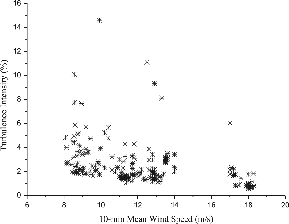
Measured turbulence intensities at 20-m height.

Figure 4.

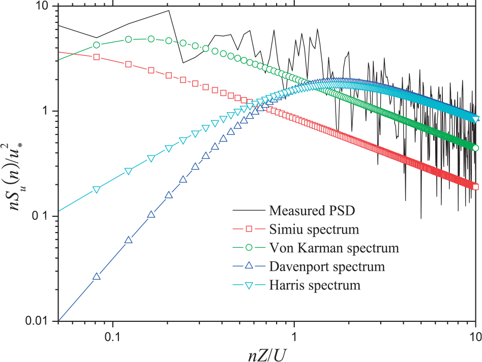
Measured and empirical power-spectral densities for the along-wind component of wind speed at 20-m height.

It is noteworthy that equations (2) and (3) are empirical formulae obtained by generalizing large quantities of data measured in different ABL wind scenarios (including sufficient moderate and high wind speed scenarios), and no wind speed limitations are specified for using these empirical formulae (Bietry et al., 1978). In this regard, the turbulence intensity profiles can be extrapolated from the single-point data measured at the engineering site of Peng-cheng electric power station under different wind speeds using equation (2). According to Figure 2, the measured turbulence intensity profile varies in a wider interval compared with the empirical turbulence intensity profile, as the upper envelope for measured turbulence intensity profiles is greater than the empirical results, but the lower envelope for measured turbulence intensity profiles is close to the coordinate axis. Thus, it can be concluded that the oncoming flow at Peng-cheng electric power station is highly uncertain, even though the ground surface roughness length is determined for the specific engineering site. The variation of the turbulence intensity observed by field measurements should be the effect of the mean wind speed which is not taken into account by the empirical formulae of the turbulence intensity profile. The comparison between measured and empirical turbulence intensity profile upper envelopes made in Figure 2 suggests that usual practice to quantify wind effects on structures based on empirical wind characteristics might be unsafe.

Overview of full-scale measurement campaign

Peng-cheng cooling towers are built in 2009 (see Figure 5). During the towers’ construction, 36 transducers are evenly installed around the principal tower’s throat section at 130-m high (see Figures 6 and 7). Besides, another transducer is arranged inside a cabin, which provides static reference pressure for measurements presented in this article.

Figure 5.

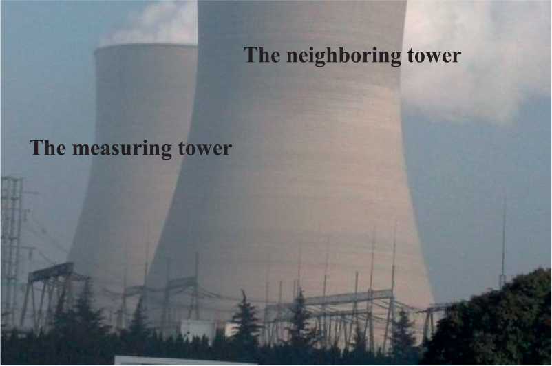
View of Peng-cheng cooling tower.

Figure 6.

Plan of pressure measurement points (m).

Figure 7.

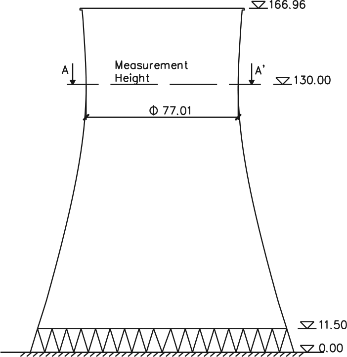
Projection of measuring tower (m).

The wind pressure transducers used are piezoresistive ones, whose dimensions are 13 cm in length, 5 cm in width, and 3 cm in depth (see Figure 8). The transducers’ maximum measured value is ±2.5 kPa (corresponding to 63 m/s wind speed). Their maximum sampling frequency and precision are 100 Hz and 1/1000 maximum range, respectively.

Figure 8.

Wind pressure transducer: (a) an actual transducer, (b) dimension (mm), and (c) a transducer installed on Peng-cheng cooling tower.

Before installed on the prototype tower, the transducer is tested for its performances in two flow fields simulated in TJ-2 wind tunnel of Tongji University, that is, a uniform flow field with negligible free-stream turbulence and an ABL turbulent flow field. TJ-2 wind tunnel is a straight-flow rectangular cross-section wind tunnel, wherein the size of the test zone is 3 m in width, 2.5 m in height, and 15 m in length. The test wind speed can be continuously controlled in a range from 0.5 to 68 m/s. Without any passive devices, the uniform flow field with negligible free-stream turbulence is obtained. The ABL turbulent flow field is obtained by means of a combination between triangular spires in the beginning of the wind tunnel’s working section and roughness elements distributed along the tunnel floor, and the turbulence intensity simulated at the height of the measurement point in turbulent flow field is around 11%. In both uniform and turbulent flow fields, the tested transducer is arranged on a metal support at the position of around 1-m high right facing the oncoming flow (see Figure 9(a)). Through tests, it is found in the uniform flow field that when oncoming flow speed is greater than 11 m/s, the noise-to-signal ratio (that is, the RMS of wind pressure divided by the mean wind pressure) for the transducer is kept below 10% (see Figure 9(b)). Besides, it is found in the turbulent flow field that the signal produced by the transducer agrees well with those obtained using high-precision electronic pressure scanning valve in 0–6 Hz frequency domain (see Figure 9(c)). These prove that the performance of the transducer is good in both time and frequency domains of interest.

Figure 9.

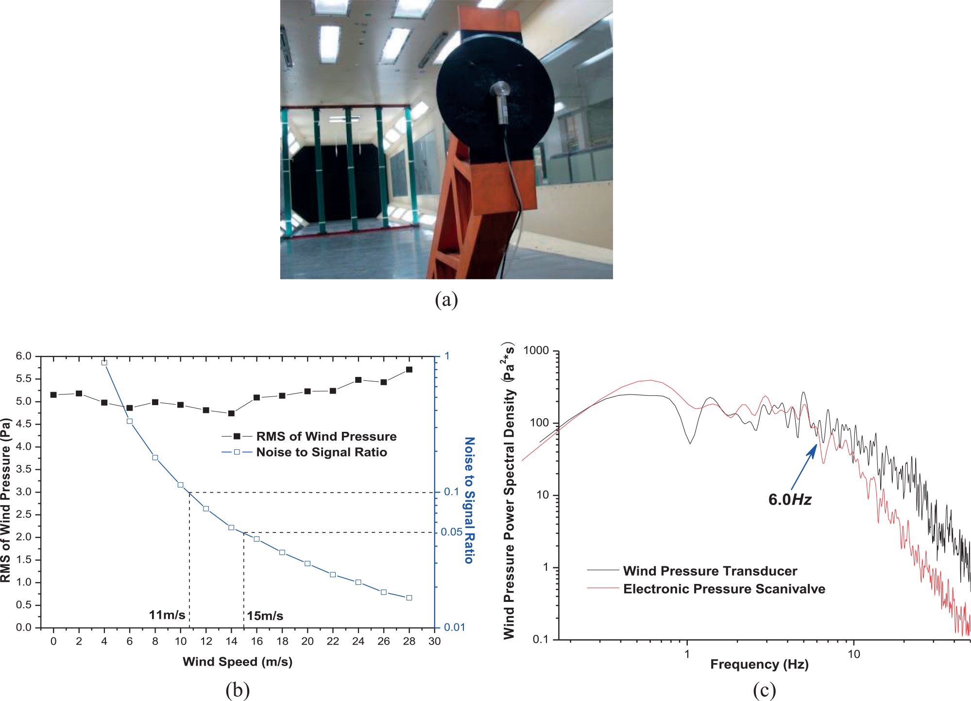
Wind tunnel tests for transducer’s performances: (a) a transducer arranged on the metal support for test, (b) static performance, and (c) dynamic performance.

The whole full-scale measurement campaign lasts from 2010 to 2015 on a 2–3 times of intensive test per year basis. In each time, we predict the occurrence of the strong wind scenario based on a local meteorological center’s weather forecast. Equipments are set up before the arrival of the strong wind, and 24-h simultaneous recordings for wind and wind-induced pressures are then conducted which usually continue for 1–2 weeks long. In the huge amount of data measured, those obtained from 28 November 2011 to 12 December 2011 are found to be most representative.

The daily predominate wind direction and the daily representative 10-min mean wind velocity obtained from 28 November 2011 to 12 December 2011 are shown in Figures 10 and 11, respectively (the mean wind velocities are obtained at 20-m high using the arranged anemometers, converted to the corresponding values at 130-m high using equation (1) and updated for the thermal convection effect). As can be seen from Figure 11, only wind speeds for 29 November and 8 December exceed 11 m/s, which represent valid strong wind scenarios. However, the wind directions on the 2 days are quite different. On 29 November, the oncoming flow is from due east, but it is from due north on 8 December (see Figure 10). Since some transducers installed on the tower’s north surface are found ineffective, complete fluctuating wind pressure distribution can only be obtained on 29 November. Besides, the upstream terrain is smooth, and there are no obvious interference effects caused by neighboring cooling towers or buildings with respect to the specific wind direction of 29 November, which can be regarded as a free-standing tower scenario. As a result, the wind-induced pressures recorded on 29 November in 2011 are used. The Re for 29 November 2011 is 6.59 × 10⁷, which falls into the transcritical Re regime.

Figure 10.

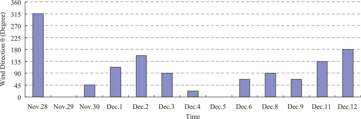
Daily predominant wind direction (see Figure 6 for definition of wind direction).

Figure 11.

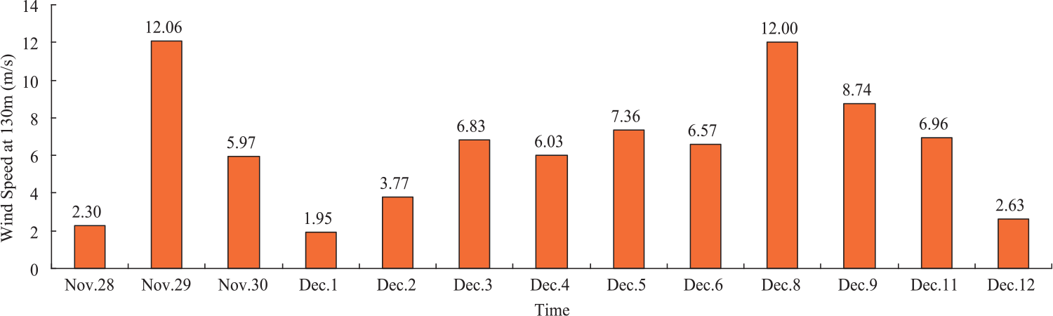
Daily representative 10-min mean wind speed at 130-m height.

Effects of free-stream turbulence on wind loads on Peng-cheng cooling tower

Three groups of 10-min wind pressure time-history samples produced by wind pressure transducers arranged on Peng-cheng cooling tower on 29 November 2011 are used in this portion of study, including one obtained under the oncoming flow with 1.54% turbulence intensity (low turbulence intensity case), another obtained under the oncoming flow with 4.23% turbulence intensity (medium turbulence intensity case), and another obtained under the oncoming flow with 10.81% turbulence intensity (high turbulence intensity case). The turbulence intensity is measured at 20-m high using the anemometer and converted to the corresponding value at 130-m high using equation (2), and the rationality of this practice can be justified by the fact that equation (2) is obtained by generalizing large quantities of data measured in different wind speed scenarios (Bietry et al., 1978), and thus universally applicable. Since the Re and the surface roughness of the cylinder are the same for the three cases, the differences in wind effects among different cases should be caused by the discrepancy of the turbulence intensity of the oncoming flow. Thus, by comparing the loading characteristics extracted from the three groups of samples, the effects of free-stream turbulence on wind loads on the actual large cooling tower can be appreciated.

Mean and fluctuating wind pressure distributions

The wind pressure on the surface of an object is represented by a dimensionless pressure coefficient. The pressure coefficient C_Pi for the ith surface measurement point on the cooling tower is defined as

C_{P i} = \frac{P_{i} - P_{\infty}}{\frac{1}{2} ρ V^{2}}

(11)

in which P_i indicates the surface wind pressure of the ith measurement point that is positive inward and negative outward; P_∞ indicates the reference static pressure; ρ and V refer to air density and oncoming flow velocity, respectively.

The mean wind pressure coefficient $μ_{m}$ is defined as

μ_{m} = \frac{\sum_{t = 1}^{n} C_{P i} (t)}{n}

(12)

The fluctuating wind pressure coefficient $σ_{μ}$ is defined as

σ_{μ} = {[\frac{1}{n} \sum_{t = 1}^{n} {(C_{P i} (t) - μ_{m})}^{2}]}^{\frac{1}{2}}

(13)

Using equations (11) to (13), the mean and fluctuating wind pressure coefficients are calculated using wind pressure samples measured on Peng-cheng cooling tower and shown in Figure 12. According to Figure 12(a), the mean wind pressure distributions obtained at different turbulence intensities almost coincide. However, fluctuating wind pressure coefficients obtained around the half-circle increase with the increase in turbulence intensity in Figure 12(b). A nonlinear relationship between the fluctuating wind pressure coefficient at stagnation $σ_{μ, θ = 0}$ and the turbulence intensity of the oncoming flow $I_{u}$ exists

σ_{μ, θ = 0} = - 11.488 {I_{u}}^{2} + 2.336 I_{u} + 0.0055

(14)

which is different from the linear empirical formula previously presented by Cheng et al. (2017b)

σ_{μ, θ = 0} = 1.517 I_{u}

(15)

Figure 12.

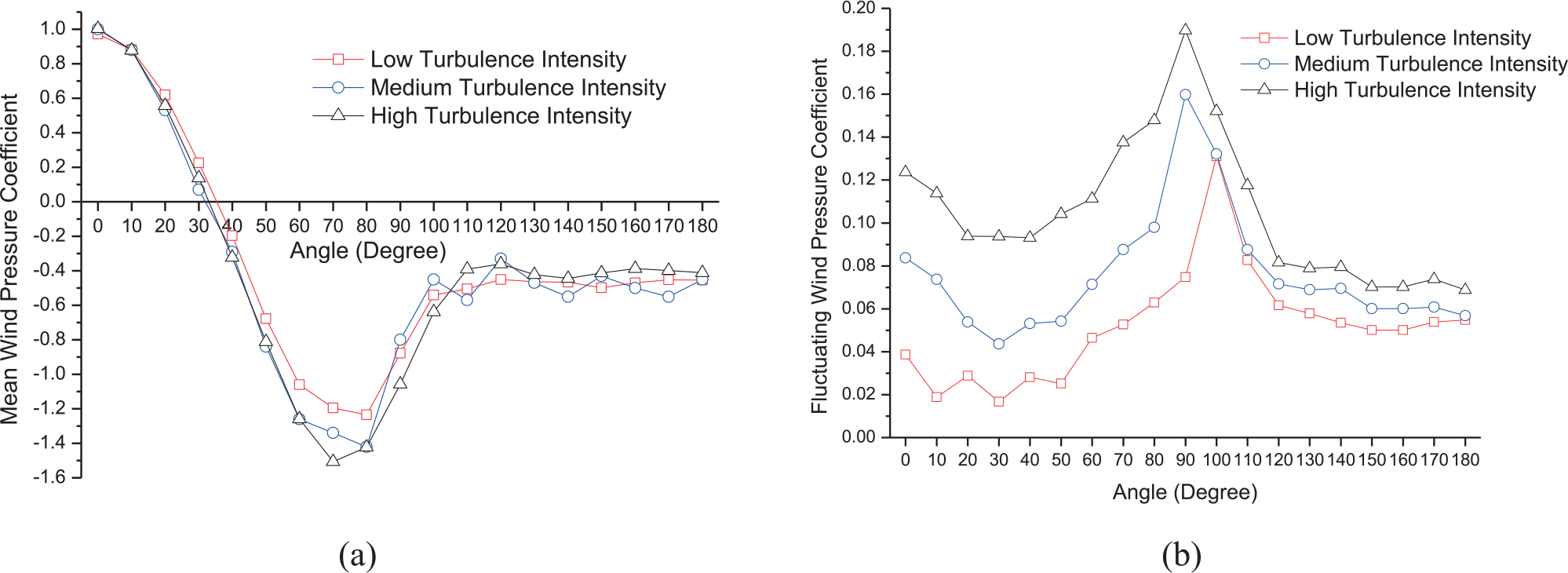
Mean and fluctuating wind pressure distributions (the abscissa refers to the included angle between the positions of the measurement point and the stagnation point, and same for Figure 13): (a) mean wind pressure distributions and (b) fluctuating wind pressure distributions.

Besides, the patterns of the fluctuating wind pressure coefficient obtained at different turbulence intensities are not exactly the same according to Figure 12(b). For the low turbulence intensity case, the shape of the fluctuating wind pressure distribution is a slightly rising slope with a sharp crest at 100°. When the turbulence intensity is increased to 10.81%, it turns into a slightly descending slope with a sharp crest at 90°, which basically agrees with the results of a previous study conducted in a wind tunnel by Zhao et al. (2017). Thus, it can be concluded that the effect of free-stream turbulence on the mean wind pressure distribution is insignificant, while that on the fluctuating wind pressure distribution is notable. This observation helps to explain the fact that most full-scale mean wind pressure distributions obtained on large cooling towers to this day are similar (see Figure 13(a)), while the full-scale fluctuating wind pressure distributions obtained are widely variable (see Figure 13(b)).

Figure 13.

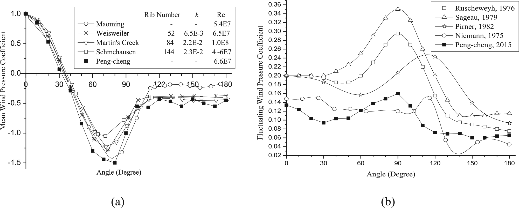
Field measurement results on different large cooling towers (reprinted from Cheng et al. (2017a)): (a) mean wind pressure distributions and (b) fluctuating wind pressure distributions.

Finally, it is noteworthy that before the separation point on the surface of the cooling tower, the influence of free-stream turbulence on the fluctuating wind pressure on the windward side is obvious. But behind the separation point, flow separation and vortex shedding will occur, and the vortex shedding may be the reason of the fluctuating wind pressure on the leeward side. According to Figure 12(b), the fluctuating wind pressure coefficients on the leeward side at different turbulence intensities are close, which indicates that the secondary turbulence caused by the vortex shedding is not related to the oncoming flow characteristics. Thus, it is possible that the vortex shedding phenomenon is unchanged at different free-stream turbulences.

Power-spectral density

The power-spectral densities of wind pressures for the three turbulence intensity cases are compared in Figure 14. According to Figure 14(a) to (d), the power-spectral densities produced at windward and side regions (0°–120°) generally increase with the increase in turbulence intensity. In particular, the power-spectral densities for the high turbulence intensity case are much greater than those for the other two cases in the high frequency range (1–6 Hz). However, the effects of free-stream turbulence on the power-spectral density are occasionally insignificant at leeward region, since the power-spectral densities obtained at 180° for low and medium turbulence intensity cases completely coincide in Figure 14(e).

Figure 14.

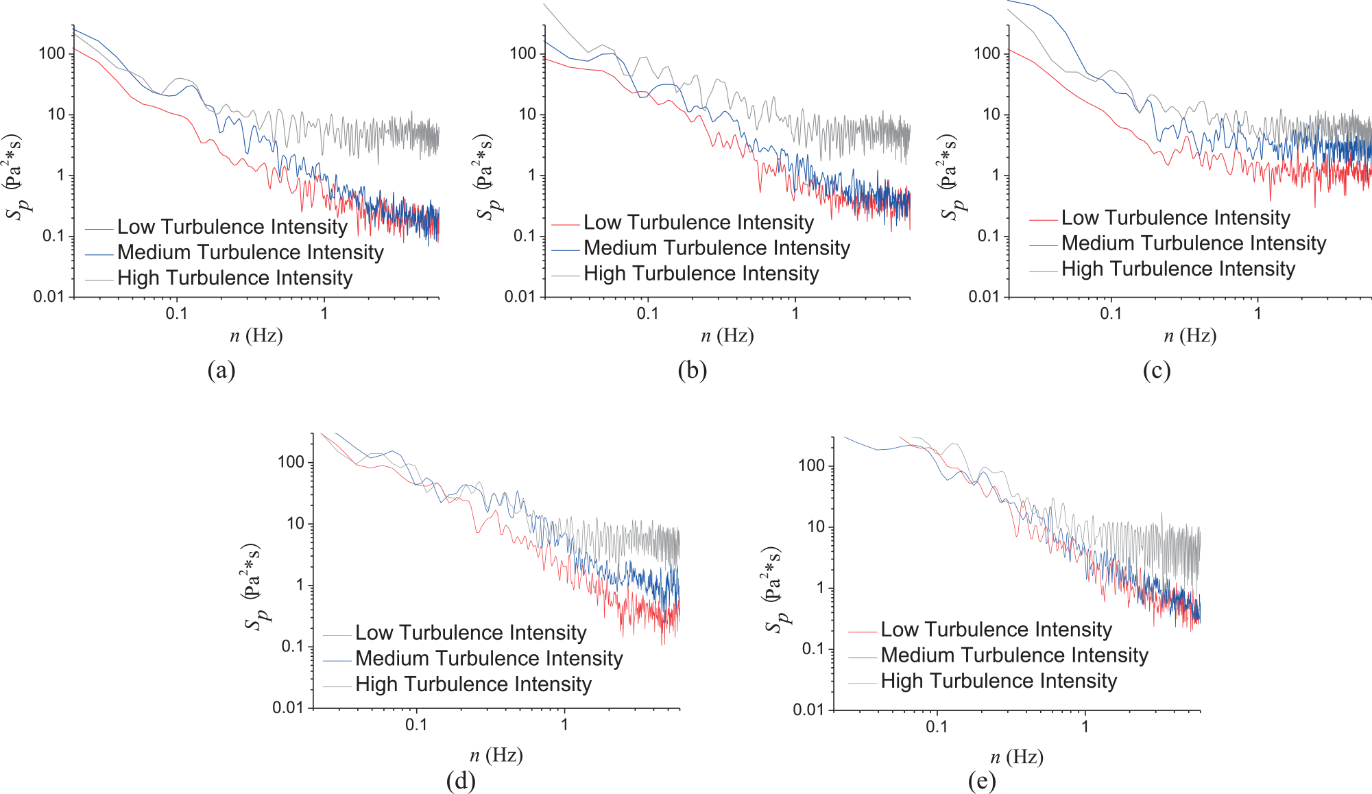
Power-spectral densities of wind pressure fluctuations (the subtitles refer to the included angle between the positions of the measurement point and the stagnation point, and same for Figures 15 to 18): (a) 20°, (b) 50°, (c) 90°, (d) 120°, and (e) 180°.

Coherence function

With respect to wind pressure coefficient fluctuations produced by two transducers both located within the region of 0°–90°, the coherence functions obtained in a flow field of low turbulence intensity are usually greater than those obtained in a flow field of high turbulence intensity in the frequency range of 0.02–0.1 Hz according to Figure 15(a) to (d). This observation suggests that the increase of free-stream turbulence weakens the coherence between wind pressures at windward and side regions in low frequency range. However, when wind pressure fluctuations are produced by transducers located far away, the effects of free-stream turbulence on the coherence function are insignificant (see Figure 15(e)). Besides, it can be noted in all subfigures of Figure 15 that the coherences for the high turbulence intensity case are dramatically strong in high frequency range (1–6 Hz), and deep-going researches are required to explain this observation.

Figure 15.

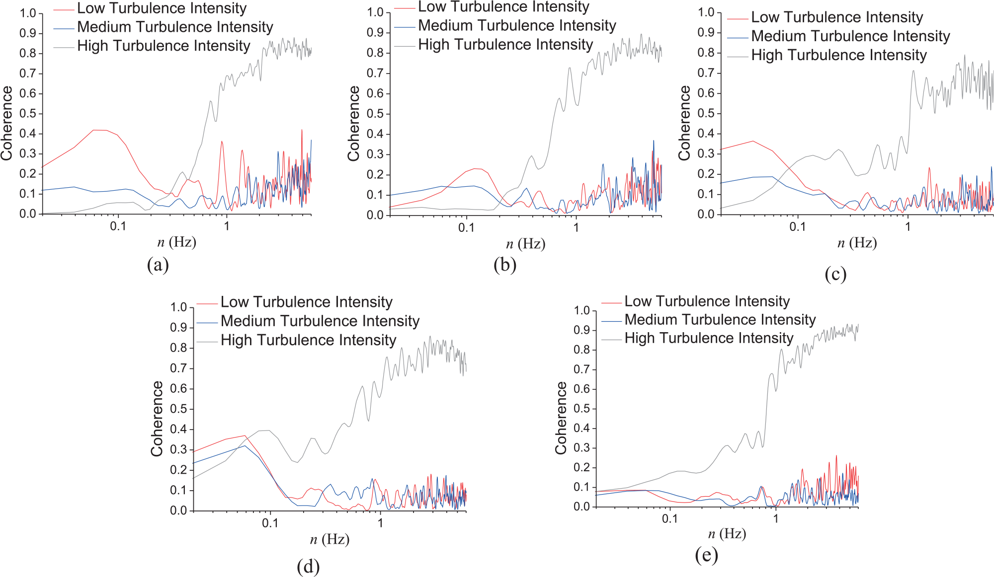
Coherence functions: (a) 20°–40°, (b) 20°–50°, (c) 20°–70°, (d) 20°–90°, and (e) 20°–120°.

Probability density function

In Figure 16, it can be found by comparing the probability density functions of the wind pressure coefficient fluctuations for the low turbulence intensity case to those for the high turbulence intensity case that the probability density functions of wind pressure fluctuations produced by all transducers change from approximately Gaussian distribution patterns to non-Gaussian patterns with the increase in free-stream turbulence. This suggests that the effects of free-stream turbulence on the probability density function are significant. Taking a step further, some probability density functions for the high turbulence intensity case are found to be more highly skewed than those for the low turbulence intensity case (see Figure 16(b), (d), and (e)) for example), corresponding to the left tails for the high turbulence intensity case containing heavier probability. Thus, the negative peak wind pressures for the high turbulence intensity case might be greater than those for the low turbulence intensity case according to Liu et al. (2009). Same situations hold true if the probability density functions for the medium turbulence intensity case are compared with those for the low turbulence intensity case.

Figure 16.

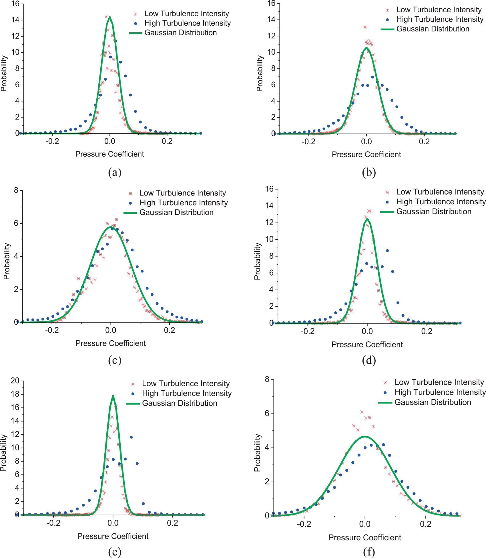
Probability density functions: (a) 20°, (b) 50°, (c) 80°, (d) 110°, (e) 140°, and (f) 180°.

Spatial correlation

The spatial correlation between two stochastic wind pressure time sequences is defined as

ρ_{x y} = \frac{E [(x - E x) (y - E y)]}{σ_{x} σ_{y}}

(16)

in which $E x$ , $E y$ and $σ_{x}$ , $σ_{y}$ are the expectations and the variances of the stochastic wind pressure time sequences $x (t)$ , $y (t)$ , respectively. Using equation (16), the spatial correlations between wind pressure coefficient fluctuations produced by transducers at different locations are calculated and presented in Figure 17. According to Figure 17, with the increase in free-stream turbulence, the spatial correlations are significantly increased for all cases. This suggests that the increase in free-stream turbulence can strengthen the spatial correlation. However, according to section “Coherence function,” the coherence between pressure time-histories produced by two transducers at different locations is usually weakened in low frequency range with the increase in turbulence intensity. The reason for this opposite observation is not clear.

Figure 17.

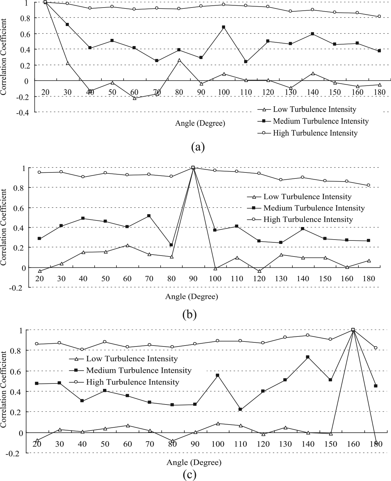
Correlation coefficients: (a) 20°—other positions, (b) 90°—other positions, and (c) 160°—other positions.

Besides, all spatial correlations for high turbulence intensity case are extremely large (greater than 0.8) according to Figure 17, which agrees with the observation presented in section “Coherence function” for high turbulence intensity case. Two possible explanations can be found for the phenomena: (1) With the increase in free-stream turbulence, the small-scale turbulence contents at different locations around the measurement section become strongly correlated. (2) When the turbulence intensity of the oncoming flow is increased to a certain level, a broadband high-frequency noise appears in the data acquisition system, which simultaneously pollutes signals in all channels. Our follow-up study will focus on confirming these possible explanations.

Validation by wind tunnel model tests

Overview of model tests

Since full-scale measurements are subjected to many uncontrollable influences, for example, the reliability of the measurement technique, the nonstationarity and the nonuniformity of the wind velocity field, the unsteadiness of the oncoming flow direction, the results of full-scale measurements presented in section “Effects of free-stream turbulence on wind loads on Peng-cheng cooling tower” should be validated for their correctness using wind tunnel model tests. The wind tunnel model tests for validation are carried out in a uniform flow field with negligible free-stream turbulence and an ABL turbulent flow field, which aim at reproducing the low and the high turbulence intensity cases described in section “Effects of free-stream turbulence on wind loads on Peng-cheng cooling tower,” respectively. TJ-3 wind tunnel at Tongji University in Shanghai, a closed circuit rectangular cross-section wind tunnel, is utilized, whose working section is 15 m in width, 2 m in height, and 14 m in length. The test wind speed can be continuously controlled in a range from 1 to 17.6 m/s in the tunnel. Without any passive devices, the uniform flow field with negligible free-stream turbulence is simulated, where the nonuniformity of wind speed in test zone is less than 1%; the average flow deviation angle is less than 0.5°; and the turbulence intensity is less than 0.5%, which is close to that of the realistic low turbulence intensity case. Using a combination between triangular spires and roughness elements, the ABL turbulent flow field for open terrain is also simulated for the test. The turbulence intensity at the height of measurement section (around 0.5 m in height) is between 10% and 10.4%, which is close to that of the realistic high turbulence intensity case.

The 1:200 scaled pressure measurement model is made of synthetic glass, which ensures its strength and rigidity. Its prototype is the 167-m high Peng-cheng cooling tower. 12 × 36 measurement points are arranged along the meridian and circumferential directions, respectively. The wind speed at the model top height is regarded as the reference wind speed, which is measured by a system composed of a pitot tube and a micromanometer. The wind pressures on the tower model are obtained using a pressure measurement system composed of a DSM3000 electronic pressure scanning valve, a PC machine, and a self-programming signal acquisition system, whose sampling frequency is 312.5 Hz. The data length at each pressure measurement point in each run is 6000.

The comprehensive high Re effects simulation method proposed by Cheng et al. (2017a) is utilized to reproduce the realistic full static and dynamic properties of the wind pressure fields on Peng-cheng cooling tower on the reduced-scale model by increasing the surface roughness of the model and adjusting the oncoming flow velocity. Eight types of surface roughness are set up on the model in both uniform and ABL turbulent flow fields. For each surface roughness condition, pressure measurement tests are conducted under four wind speeds (6, 8, 10, and 12 m/s). Thus, the data for a total of 32 (8 × 4) cases are obtained in each flow field. To avoid the end effects, the eigth circumferential section which is closest to the throat of the tower model is chosen as the study section. By processing data obtained on the eighth section, results of 32 cases are obtained for both uniform flow field and ABL turbulent flow field. It is found that only 5 within the 32 cases can successfully re-simulate the actual mean wind pressure distributions of Peng-cheng cooling tower in the reduced-scale model with lower Re in both two flow fields, and they are selected as the candidate simulation cases. Then, comparing the fluctuating wind pressure distributions of the candidate simulation cases to the results measured on Peng-cheng cooling tower, it can be found that for both mean and fluctuating wind pressure distributions, the optimum high Re effects simulation cases are a model with two-layer paper tape and a + 10 m/s wind speed for uniform flow field and a model with four-layer paper tape and a + 6 m/s wind speed for ABL turbulent flow field. The data obtained for the two optimum cases are truthful representations of the realistic wind effects for high and low turbulence intensity cases. After data processing, the power-spectral densities, the coherence functions, the probability density functions, and the correlation coefficients of the fluctuating wind pressure coefficients are respectively extracted.

Model test results

Characteristics of wind effects obtained on the reduced-scale model in uniform and turbulent flow fields are compared in Figure 18. According to Figure 18(a), the power-spectral density increases with the increase in free-stream turbulence over the full frequency domain in windward side, which agrees with those obtained in section “Power-spectral density” for full-scale measurement studies. The coherence functions between wind pressure fluctuations obtained at 20° and 40° on the reduced-scale model in the two flow fields are shown in Figure 18(b), which support the observation reported in section “Coherence function” that the increase of free-stream turbulence weakens the coherence between wind pressures at windward region in low frequency range. Figure 18(c) and (d) presents the probability density functions obtained at two locations on the model’s throat section. As can be seen, the probability density functions change from approximately Gaussian distribution patterns to non-Gaussian patterns with the increase in free-stream turbulence, which agrees with the finding presented in section “Probability density function.”Figure 18(e) shows the correlation coefficients between wind pressure fluctuations at 140° and other positions on the model. It is obvious that the correlation coefficients are increased with the increase in free-stream turbulence for most cases, which agrees with the observation presented in section “Spatial correlation.”

Figure 18.

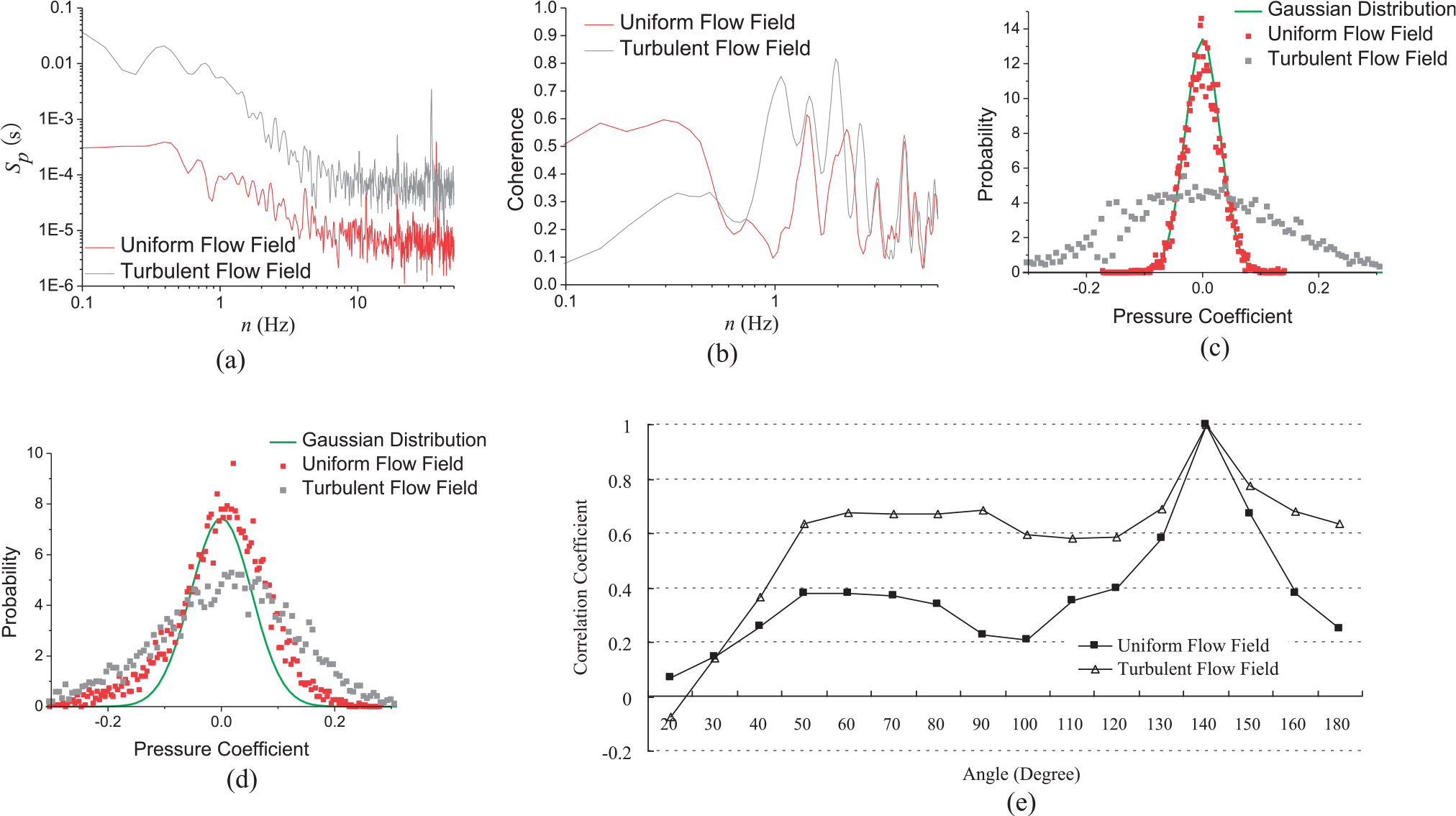
Characteristics of wind effects obtained on the tower model: (a) power-spectral densities of wind pressure coefficient fluctuations at 20°, (b) coherence functions between wind pressure coefficient fluctuations at 20° and 40°, (c) probability density functions of wind pressure coefficient fluctuations at 30°, (d) probability density functions of wind pressure coefficient fluctuations at 120°, and (e) correlation coefficients between wind pressure coefficient fluctuations at 140° and other positions.

Conclusion

Empirical natural wind characteristics suggest that the turbulence intensity profile cannot be definitively described for each terrain type, since the variation of the turbulence intensity is induced by the variation of the ground surface roughness length. However, meteorological wind measurements conduct at Peng-cheng electric power station suggest that the variability of the measured turbulence intensity is even stronger for a determined ground surface roughness length. The variation observed on the location should be the effect of the mean wind speed according to Quan et al. (2013) and our research, which is not taken into account by the empirical formulae of the turbulence intensity profile presented in Codes of Practice and monographs. It is thus indicated that there exist possibilities that the empirical natural wind characteristics presented in Codes of Practice and monographs might not be applicable to a realistic engineering site. A reasonable explanation is that the empirical knowledge is obtained by generalizing large quantities of measured data, and simplifications are usually included in generalization.

Since the ABL turbulence is highly variable, it is of practical significance to quantify the effects of free-stream turbulence on wind loads on large structures. Based on the field measurement campaign for wind effects on Peng-cheng cooling tower, it is found that the turbulence intensity of the ABL flow has little effects on the static wind loads on the full-scale cooling tower, but it significantly influences the dynamic wind effects in most cases. Wind effects obtained in a flow field of high turbulence intensity are generally more unfavorable than those obtained in a flow field of low turbulence intensity, so the practice to quantify wind effects on cooling towers for either wind-engineering design or research should be based upon a case of sufficient turbulence intensity for conservativeness.

A further step is taken to employ wind tunnel model tests to validate the full-scale measurement results. Realistic ABL wind events with high and low turbulence intensities are both re-simulated in the wind tunnel based on a two-level simulation strategy according to Cermak (1987): first, similarity of the desired natural wind characteristics is achieved in the wind tunnel with/without passive simulation devices; second, similarity of the specific wind effects is achieved on the reduced-scale model utilizing the comprehensive high Re effects simulation method proposed by Cheng et al. (2017a). It is found that most results obtained in the wind tunnel qualitatively agree with the findings based on field measurements, although some discrepancies can be observed if the model test results are directly used to compare with the corresponding full-scale measurement results.

Footnotes

Declaration of Conflicting Interests

The author(s) declared no potential conflicts of interest with respect to the research, authorship, and/or publication of this article.

Funding

The author(s) disclosed receipt of the following financial support for the research, authorship, and/or publication of this article: The authors gratefully acknowledge the supports of the National Natural Science Foundation of China (51178353 and 50978203), the National Key Basic Research Program of China (i.e. 973 Program) (2013CB036300), and China Postdoctoral Science Foundation.

References

Achenbach

(1968) Distribution of local pressure and skin friction around a circular cylinder in cross-flow up to Re = 5 × 10⁶. Journal of Fluid Mechanics 34(4): 625–639.

Armitt

(1980) Wind loading on cooling towers. Journal of the Structural Division 106(3): 623–641.

Bearman

(1968) The Flow Around a Circular Cylinder in the Critical Reynolds Number Regime (NPL Aero Report No. 1257). Teddington: Aerodynamics Division, National Physical Laboratory.

Bietry

Sacre

Simiu

(1978) Mean wind profiles and change of terrain roughness. Journal of the Structural Division 104(10): 1585–1593.

Cermak

(1987) Advances in physical modeling for wind engineering. Journal of Engineering Mechanics 113: 737–756.

Cheng

Zhao

et al . (2017a) A comprehensive high Reynolds number effects simulation method for wind pressures on cooling tower models. Wind & Structures 24(2): 119–144.

Cheng

Zhao

et al . (2017b) Wind effects on rough-walled and smooth-walled large cooling towers. Advances in Structural Engineering 20(6): 843–864.

Cheung

JCK

Melbourne

(1983) Turbulence effects on some aerodynamic parameters of a circular cylinder at supercritical Reynolds numbers. Journal of Wind Engineering & Industrial Aerodynamics 14: 399–410.

Cook

(1997) The Deaves and Harris ABL model applied to heterogeneous terrain. Journal of Wind Engineering & Industrial Aerodynamics 66: 197–214.

10.

DL/T 5339-2006:2006 (2006) Technical specification for hydraulic design of thermal power plant (in Chinese).

11.

Dragoiescu

Xie

Kelly

(2011) Reynolds number effects on a super-tall tower with rounded triangular shape. In: Proceedings of the 13th international conference on wind engineering, Amsterdam, 10–15 July 2011.

12.

Drew

Barlow

Lane

(2013) Observations of wind speed profiles over greater London, UK, using a Doppler lidar. Journal of Wind Engineering & Industrial Aerodynamics 121: 98–105.

13.

EN 1991-1-4: 2004 (2004) Eurocode 1: actions on structures—part 1–4: general actions—wind actions.

14.

ESDU 01008:2005 (2005) Computer program for wind speeds and turbulence properties: flat or hilly sites in terrain with roughness changes.

15.

GB 50009-2001:2002 (2002) Load code for the design of building structures (in Chinese).

16.

GB/T 50102-2003:2003 (2003) Code for design of cooling for industrial recirculating water (in Chinese).

17.

Gualtieri

(2017) Wind resource extrapolating tools for modern multi-MW wind turbines: comparison of the Deaves and Harris model vs. the power law. Journal of Wind Engineering & Industrial Aerodynamics 170: 107–117.

18.

Holmes

(2001) Wind Loading of Structures. London: Spon Press.

19.

Kiya

Suzuki

Arie

et al . (1982) A contribution to the free-stream turbulence effect on the flow past a circular cylinder. Journal of Fluid Mechanics 115: 151–164.

20.

Liu

Prevatt

Aponte-Bermudez

et al . (2009) Field measurement and wind tunnel simulation of hurricane wind loads on a single family dwelling. Engineering Structures 31: 2265–2274.

21.

Matsuda

Cooper

Tanaka

et al . (2001) An investigation of Reynolds number effects on the steady and unsteady aerodynamic forces on a 1:10 scale bridge deck section model. Journal of Wind Engineering & Industrial Aerodynamics 89: 619–632.

22.

Niemann

(1971) Zur Stationaren Windbelastung Rotations-symmetrischer Bauwerke Im Bereich Transkritischer Reynoldszahlen (in German). Bochum: Ruhr-Universität Bochum.

23.

Niemann

Hölscher

(1990) A review of recent experiments on the flow past circular cylinders. Journal of Wind Engineering & Industrial Aerodynamics 33(1): 197–209.

24.

Niemann

Pröpper

(1975) Some properties of fluctuating wind pressures on a full-scale cooling tower. Journal of Industrial Aerodynamics 1: 349–359.

25.

Niemann

Ruhwedel

(1980) Full-scale and model tests on wind-induced, static and dynamic stresses in cooling tower shells. Engineering Structures 2(2): 81–89.

26.

Pirner

(1982) Wind pressure fluctuations on a cooling tower. Journal of Wind Engineering & Industrial Aerodynamics 10: 343–360.

27.

Quan

Wang

et al . (2013) Field measurement of wind speeds and wind-induced responses atop the Shanghai world financial center under normal climate conditions. Mathematical Problems in Engineering 2013: 902643

28.

Richards

Norris

(2015) Appropriate boundary conditions for a pressure driven boundary layer. Journal of Wind Engineering & Industrial Aerodynamics 142: 43–52.

29.

Roshko

(1961) Experiments on the flow past a circular cylinder at very high Reynolds number. Journal of Fluid Mechanics 10(3): 345–356.

30.

Ruscheweyh

(1975) Wind loadings on hyperbolic natural draught cooling towers. Journal of Industrial Aerodynamics 1: 335–340.

31.

Simiu

Scanlan

(1996) Wind Effects on Structures. New York: John Wiley & Sons.

32.

Sollenberger

Scanlan

(1974) Pressure-difference measurements across the shell of a full-scale natural draft cooling tower. In: Proceedings of the symposium on full-scale measurements of wind effects, University of Western Ontario, London, ON, Canada, 23–29 June 1974.

33.

Sun

Zhou

(1983) Wind pressure distribution around a ribless hyperbolic cooling tower. Journal of Wind Engineering & Industrial Aerodynamics 14: 181–192.

34.

Surry

(1972) Some effects of intense turbulence on the aerodynamics of a circular cylinder at subcritical Reynolds number. Journal of Fluid Mechanics 52: 543–563.

35.

Tieleman

(2008) Strong wind observations in the atmospheric surface layer. Journal of Wind Engineering & Industrial Aerodynamics 96: 41–77.

36.

Zhao

Kareem

(2017) Fluctuating wind pressure distribution around full-scale cooling towers. Journal of Wind Engineering & Industrial Aerodynamics 165: 34–45.