
Abstract
In this article, an analytical moment-based procedure is developed for estimating the first passage probability of stationary non-Gaussian structural responses for practical applications. In the procedure, an improved explicit third-order polynomial transformation (fourth-moment Gaussian transformation) is proposed, and the coefficients of the third-order polynomial transformation are first determined by the first four moments (i.e. mean, standard deviation, skewness, and kurtosis) of the structural response. The inverse transformation (the equivalent Gaussian fractile) of the third-order polynomial transformation is then used to map the marginal distributions of a non-Gaussian response into the standard Gaussian distributions. Finally, the first passage probabilities can be calculated with the consideration of the effects of clumping crossings and initial conditions. The accuracy and efficiency of the proposed transformation are demonstrated through several numerical examples for both the “softening” responses (with wider tails than Gaussian distribution; for example, kurtosis > 3) and “hardening” responses (with narrower tails; for example, kurtosis < 3). It is found that the proposed method has better accuracy for estimating the first passage probabilities than the existing methods, which provides an efficient and rational tool for the first passage probability assessment of stationary non-Gaussian process.
Keywords
Introduction
The failure of a random dynamic system is usually defined based on the exceedance of a predefined critical threshold level. In many engineering applications, it is important to calculate the probabilities that a structural response exceeds the critical threshold levels in the given time interval [0, T]. The critical threshold level could be the yield stress, strain, or displacement. Failure occurs when the critical threshold value is exceeded at its first time, and this kind of analysis falls into the category of the first passage problem (Coleman, 1959; Lin, 1970; Rice, 1944, 1945; Vanmarcke, 1975).
So far, there are no simple analytical solutions existing for the first passage problem even for the simplest case, that is, a single-degree-of-freedom (SDOF) linear oscillator subject to Gaussian white noise excitation with a deterministic failure threshold (Crandall, 1970; Naess, 1990). Many numerical studies have been devoted to the computation of the first passage probability (Au and Beck, 2001a, 2001b; Naess et al. 2010; Naess and Gaidai, 2009), and the Monte Carlo simulation (MCS) is the most general and robust, although it is also computationally expensive for low-probability events. For analytical studies, it has also been devoted to estimate the first passage probability (Barbato and Conte, 2011; Coleman, 1959; Ghazizadeh et al., 2012; Lin, 1970; Rice, 1944, 1945; Vanmarcke, 1975), and the Poisson approximation is the most widely used. In most cases, the computation of the first passage probability is often based on the up-crossing approach which assumes that the crossings are independent and the responses are Gaussian.
The well-known Gaussian model is generally inappropriate for calculating the first passage probability of a structure when structural behavior is non-linear, or the excitation is non-Gaussian (e.g. wind and wave loads). Structural responses generally cannot be modeled as Gaussian stochastic processes for these cases. This is important particularly for non-Gaussian response whose tail behavior is different from Gaussian responses. Series distribution methods (Grigoriu, 1984; Ochi, 1986) can be used to transform known statistical results (such as mean up-crossing rates and extreme values of a Gaussian process) into those of a non-Gaussian process by finding a simple functional transformation of the equivalent Gaussian statistics. For these cases, various non-linear models have been formulated through series approximation to map a non-Gaussian response process into a standard Gaussian one. For example, full probability distributions have been estimated from response moments (e.g. mean, standard deviation, skewness, and kurtosis) with Gram–Charlier and Edgeworth series (Johnsom and Kotz, 1970). These series, however, can yield multi-modal and even negative probability densities and crossing rates. Winterstein (1988) proposed Hermite moment models known as Winterstein’s polynomials (see Appendix 1) using response moments in terms of Hermite polynomials to form non-Gaussian response contributions. Winterstein’s polynomials offers equivalent Gaussian fractile mapping between Gaussian and non-Gaussian processes and has been widely used (Jensen, 1994; Puig and Akian, 2004; Winterstein and Kashef, 2000; Winterstein and Mackenzie, 2011). Winterstein’s polynomials, however, cannot be directly applied to some processes (Choi and Sweetman, 2010) since the transformation is non-monotonic for certain combinations of skewness and kurtosis (Low, 2013) and is known to have poor accuracy for strongly non-Gaussian processes (Ding and Chen, 2014). Based on Winterstein’s polynomials, the first passage probability for stationary non-Gaussian response with the consideration of the effects of clumping and initial conditions on the up-crossing rate has been proposed by He and Zhao (2007). However, significant difference was observed between the results based on Winterstein’s polynomials and those from MCS method, especially for the case of “hardening” responses (with narrower tails; for example, kurtosis < 3) due to transformation errors. Moreover, unlike the “softening” responses (with wider than Gaussian distribution tails; for example, kurtosis > 3) of Winterstein’s polynomials, the relationship between statistical moments and Hermite model coefficients cannot be formulated in closed form (Ding and Chen, 2016). Further research is, therefore, necessary to improve the accuracy of transforming the stationary non-Gaussian processes to Gaussian ones. Although the reliability problem where the discrete load process (such as a Poisson process) is also studied in some relevant references (Wang et al., 2016; Wang and Zhang, 2018), it is should be noted that the focus of this article is on the reliability problem subject to a continuous load process.
The objective of this article is to propose a new transformation approach properly for both the “softening” and “hardening” responses to calculate the first passage probabilities of stationary non-Gaussian structural responses. This article is organized as follows. In the next section, the formulation of the first passage probabilities of stationary non-Gaussian structural responses is described; in section “The third-order polynomial transformation for the first passage probability assessment of stationary non-Gaussian process”, the third-order polynomial transformation is developed to approximate stationary non-Gaussian structural responses and for practical applications, an explicit third-order polynomial transformation (fourth-moment Gaussian transformation) is proposed based on comparison studies of transformation methods, and its inverse transformation (the equivalent Gaussian fractile) is then derived to map a non-Gaussian structural response into a standard Gaussian process; in section “Numerical examples”, the accuracy and efficiency of this transformation for both “softening” responses and “hardening” responses are demonstrated through several numerical examples; finally, the findings of this article are summarized in the conclusions. It is believed that the methodology presented in this article provides an efficient and rational tool for the first passage probability assessment of stationary non-Gaussian process.
Formulation of the first passage probability of stationary non-Gaussian structural responses
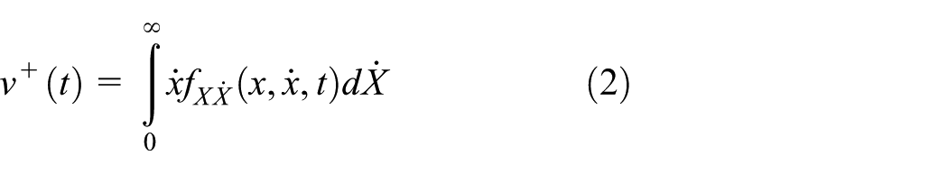
In the structural safety analysis, one often assumes that the crossing of a random response follow the Poisson distribution and the first passage probability, Pf(T) is given by (Coleman, 1959)

where
where

where

where
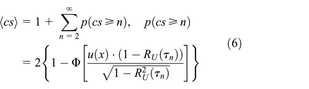
This approach has been proved to be exact for very high critical levels (Cramér, 1966). If X(t) is narrow-banded or the critical threshold level is low, the clumping effect of the up-crossing events should be considered to modify the mean level up-crossing rates in equation (2) (He, 2009, 2015). Since the exceedances of the critical threshold level tend to occur in clumps, the clump size

where

For high critical level, equation (1) can be improved as (Ditlevsen, 1986)
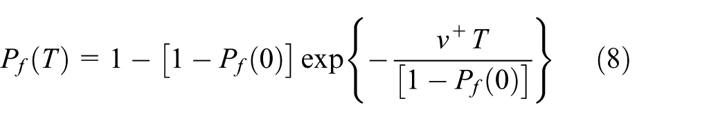
where Pf(0) is the probability of instantaneous failure at T = 0;
The first passage probabilities were investigated by He and Zhao (2007) for stationary non-Gaussian structural responses using equations (5) to (8), in which the equivalent Gaussian fractile u(x) based on Winterstein’s polynomials was adopted. However, significant differences were observed between the results based on Winterstein’s polynomials and those estimated using the MCS method, especially for the case of “hardening” responses due to the transformation errors of Winterstein’s polynomials. In the next section, the third-order polynomial transformation is proposed to solve this problem.
The third-order polynomial transformation for the first passage probability assessment of stationary non-Gaussian process
The third-order polynomial transformation and its inverse function
The third-order polynomial transformation method suggested by Fleishman (1978) can be formulated as
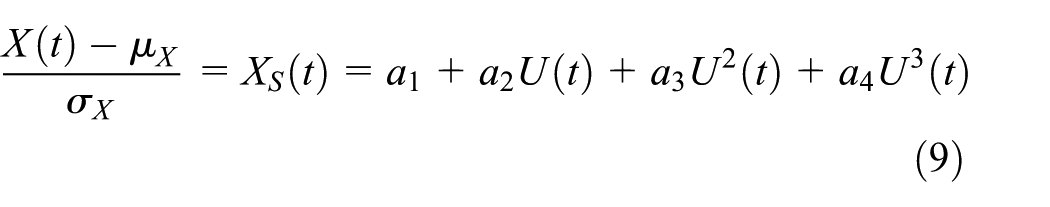
where X(t) is a stochastic process; XS(t) is standardized stochastic process;
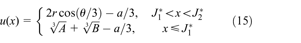
Once the four coefficients determined and considering the critical threshold level x, the inverse transformation (the equivalent Gaussian fractile) u(x) of the third-order polynomial transformation can be expressed as follows (Zhang et al., 2018; Zhao and Lu, 2007):
When a4 > 0 and

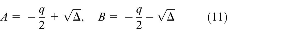
where A, B, and a are the parameters, and they are expressed as follows
When a4 > 0,

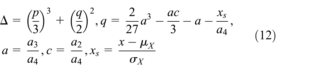
where

When a4 > 0,
When a4 < 0

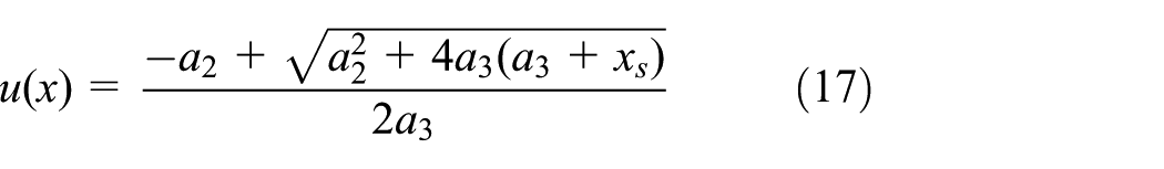
When a4 = 0 and a3 ≠ 0
When a4 = a3 = 0

Combined with equations (5) to (8) and the inverse transformation (the equivalent Gaussian fractile) of the third-order polynomial transformation u(x) given by equations (10), (13), and (15) to (18), an analytical moment-based procedure based on the third-order polynomial transformation is developed for calculating the first passage probability of a stationary non-Gaussian process.
An improved explicit third-order polynomial transformation and its inverse function
As the determination of the four coefficients of equation (9) is not easy, the solution of non-linear equations has to be found. Therefore, it is attractive for practical applications to have the approximate but explicit formulae for the four coefficients in equation (9).
In order to avoid the solution of non-linear equations, Zhao and Lu (2007) proposed a simple explicit third-order polynomial function, which was developed from a large amount of data of third and fourth dimensionless central moments through trial and error

where the coefficients
and
It was shown that equations (19) to (21) can give fairly good approximation of equation (9) when
The four polynomial coefficients determined by equations (19) to (21) are illustrated and compared with exact values obtained by non-linear equations (Zhao and Lu, 2007) in Figure 1. The coefficients are expressed as functions of

Fitting and validation of polynomial coefficients for the proposed model.
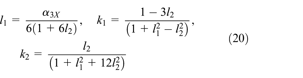
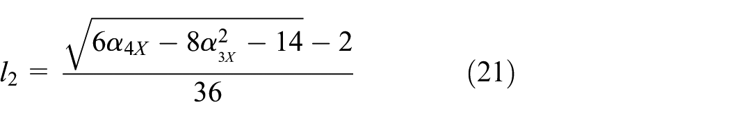
In this study, an improved version of equation (20) is developed from a large amount of data of third and fourth dimensionless central moments through trial and error. The development procedure is simply described as: for a given skewness α3X and different kurtosis α4X of XS(t), a set of polynomial coefficients (accurate value) can be determined by making the first four moments of the left side of equation (9) equal to those of the right side (Fleishman, 1978; Zhao and Lu, 2008); Then, using regression analysis, the polynomial coefficients as functions of skewness α3X and kurtosis α4X can be obtained as follows
When |α3X| ⩽ 1.2, equations (20) and (21) are still applicable, while when
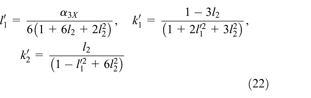
where
The four polynomial coefficients determined by equation (22) and Winterstein’s polynomials (Winterstein, 1988) are also illustrated in Figure 1. As can be observed from Figure 1 that (1) coefficients of Winterstein’s polynomials have the largest differences from the accurate coefficients and (2) coefficients obtained using equation (22) are in close agreement with the accurate ones throughout the entire investigation range.
According to equations (10) to (18), the inverse transformation or equivalent Gaussian fractile u(x) based on the improved explicit third-order polynomial transformation (equations (19) to (22)) can be readily obtained through replacing a1, a2, a3, and a4 by −l1, k1, l1, and k2 or
The first passage probability assessment of stationary non-Gaussian process based on the third-order polynomial transformation
According to the description of sections “Formulation of the first passage probability of stationary non-Gaussian structural responses” and “The third-order polynomial transformation for the first passage probability assessment of stationary non-Gaussian process”, the procedure for calculating the first passage probability of a stationary non-Gaussian process based on the third-order polynomial transformation is described as follows, with the flowchart illustrated in Figure 2:
Estimate the first four moments of a stationary non-Gaussian process.
Determine the critical threshold level x of a stationary non-Gaussian process.
After the first four moments of a stationary non-Gaussian process and the critical threshold levels x have been given, the equivalent Gaussian fractile based on the explicit third-order polynomial transformation can be estimated by equations (10) to (18), where the coefficients a1, a2, a3, and a4 are replaced by −l1, k1, l1, and k2 or
Compute the first passage probability of a stationary non-Gaussian process using equations (5) to (8).

Flowchart of procedure for calculating the first passage probability of a stationary non-Gaussian process.
Numerical examples
To investigate the accuracy and efficiency of the proposed explicit third-order polynomial transformation, the x–u transformations of three different distributions including “softening” responses (
x–u transformations using the first four moments of non-normal random variables
Example 1: the investigation of the proposed x–u transformations
In evaluating a normal transformation technique, the first concern could be how the relation between non-normal and normal variables is described by the technique. Suppose a random variable x is known to have a PDF, f(x), the x–u transformation can be obtained using the proposed fourth-moment standardization function or the other normal transformation techniques. Since the Rosenblatt transformation (Hohenbichler and Rackwitz, 1981) completely preserves the known marginal distribution, that is, F(x) = Φ(u), it is used herein as the benchmark in performance evaluation for the other normal transformation techniques.
Three random variables with different distributions, that is, Gumbel distribution, log-normal distribution, and truncated normal distribution, are considered in the first example. The parameters of the three distributions and their first four moments are listed in Table 1. From Table 1, Case 1 is a “softening” response with kurtosis = 5.4 (>3) and
In Figure 3, the transformation function obtained using Winterstein’s polynomials provides good results when the absolute value of xs is small, while when the absolute value of xs is large, the results obtained from Winterstein’s polynomials differ greatly from those obtained using the Rosenblatt transformation.
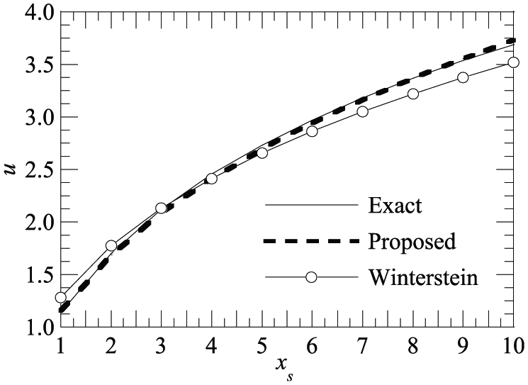
In Figure 4, the transformation function based on Winterstein’s polynomials yields significant errors in almost the whole investigation range, compared with those obtained using the Rosenblatt transformation. The errors come from the transformation error of Winterstein’s polynomials especially when the absolute value of
Again, it can be clearly observed from Figure 5 that the transformation function obtained using Winterstein’s polynomial has significant difference from those obtained using the Rosenblatt transformation when the absolute value of xs is large.
The proposed method shows better accuracy than Winterstein’s polynomials. The results obtained from the proposed transformation coincide with those of the Rosenblatt transformation throughout the entire investigation range, which further demonstrate the accuracy and efficiency of the proposed polynomial coefficients in the previous section.
The probability distributions and their first four moments for Example 1.
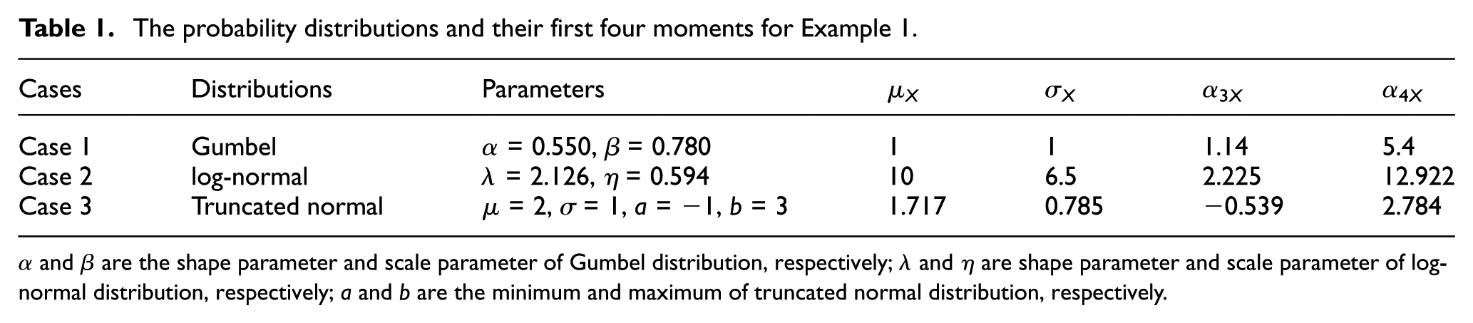
α and β are the shape parameter and scale parameter of Gumbel distribution, respectively; λ and η are shape parameter and scale parameter of log-normal distribution, respectively; a and b are the minimum and maximum of truncated normal distribution, respectively.
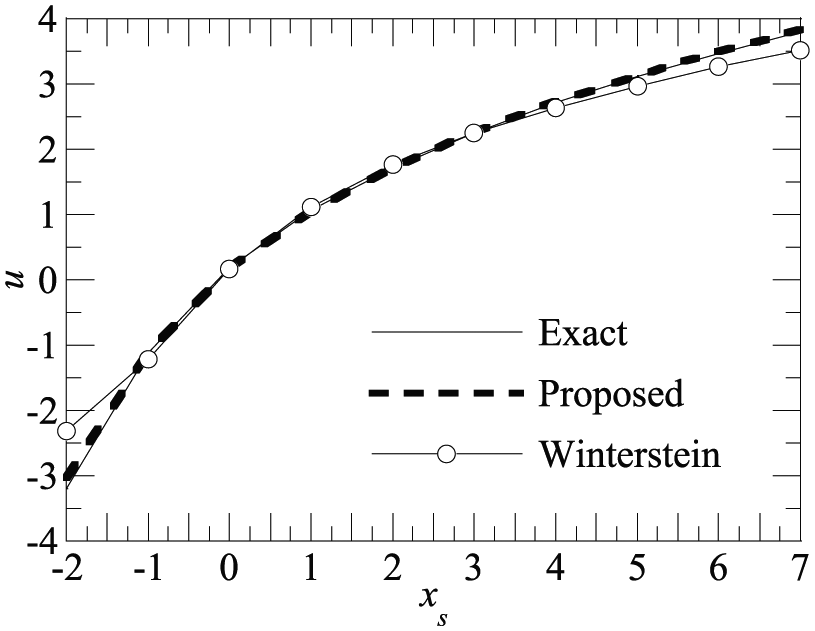
x–u transformations of Gumbel distribution in Example 1.

x–u transformations of log-normal distribution in Example 1.
x–u transformations of truncated normal distribution in Example 1.
Application in first passage probability assessment of stationary non-Gaussian process
Example 2: first passage probabilities of softening responses
The second example considers a linear SDOF structure excited by a quadratic forcing function F(t) as shown in Figure 6. Specifically, it is assumed that the forcing function is F(t) = α1U(t) + α2U2(t), where U(t) is a stationary, zero-mean Gaussian process, and α1 and α2 are constants. This example is chosen primarily for its simplicity, but a similar forcing function could, for instance, serve as a model for dynamic wind pressure, although with parameters different from those chosen here.
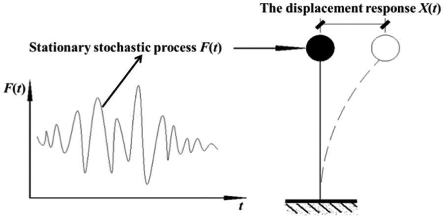
A single-degree-of-freedom (SDOF) structure excited by a quadratic forcing function F(t) for Example 2.
According to Naess (1987), the non-Gaussian structural response, X(t), to the excitation force F(t) is

where
Equation (23) gives the known second-order stochastic Volterra series solution of the considered non-linear dynamic system. How to use numerical calculation to obtain statistical moments of the stationary responses of the non-linear dynamical system can be found in Naess (1987).
In this example, it is assumed that
Using the first four moments of the quadratic part of the responses, the first passage probabilities of stationary non-Gaussian structural responses for critical threshold level x = 4.5σX and x = 5σX obtained using the proposed method are shown in Figure 7(a) and (b), respectively, compared with the results obtained by assuming Gaussian model, the method proposed by He and Zhao (2007), and the MCS method (Au and Beck, 2001b; Bayer and Bucher, 1999). From Figure 7(a) and (b):
The results of Gaussian model have the greatest differences from those of MCS method (with 100,000 samples) and are too conservative.
Although the method by He and Zhao (2007) improves the Gaussian model, its results are still somewhat quite different from those by MCS method. The difference comes from transformation errors of Winterstein’s polynomials, to which the first passage probability has large sensitivity.
The proposed method performs better than the method by He and Zhao (2007), and the obtained results are in close agreement with those by MCS method during the whole interval T. Therefore, for “softening” responses, the proposed procedure is more suitable for engineering applications.
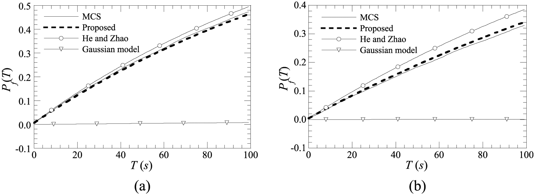
The first passage probabilities of structural responses in Example 2: (a) x = 4.5σX and (b) x = 5σX.
Example 3: first passage probabilities of hardening responses
The third example considers a Duffing oscillator subjected to a stationary Gaussian white noise. The structural response X(t) due to the excitation f(t) is determined by the following equation

where ε is a parameter for denoting the non-linearity of the restoring force; and f(t) is a zero-mean stationary Gaussian white noise. Using Fokker-Planck-Kolmogorov (FPK) equation method (Crandall, 1958), the PDF of non-linear displacement responses, p(X), can be expressed as
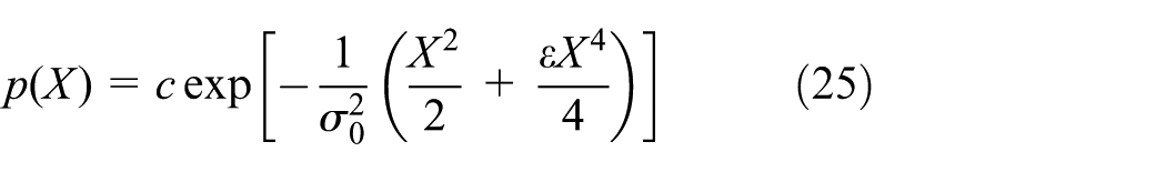
in which
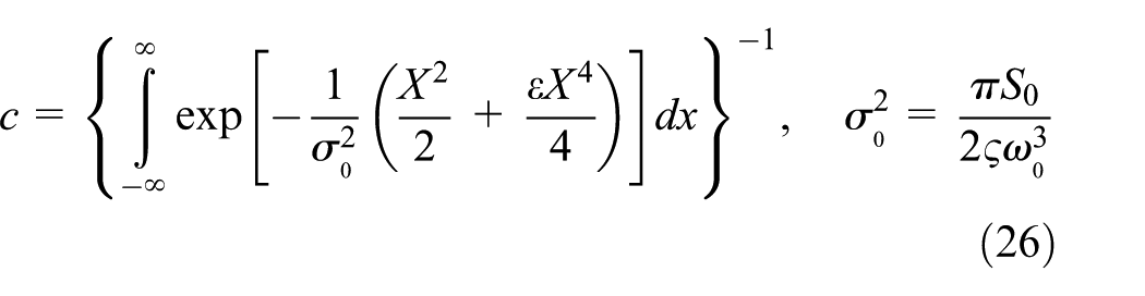
The functional form of p(X) demonstrates that X(t) is non-Gaussian. Assuming that S0 = 1 m2s, ω0 = 2 rad/s, ς = 0.05, and ε = 0.5, the structural parameters and the first four moments of displacement response can be readily determined by equations (25) and (26) and are µX = 0, σX = 1.203, α3X = 0, and α4X = 2.369, respectively. The structural responses for this example is a “hardening” responses since α4X = 2.369 < 3. Considering the critical threshold level of x = 2σX, the variations of the first passage probability with regard to excitation time T obtained by using the proposed method are illustrated in Figure 8, together with the results obtained by assuming Gaussian model, the method proposed by He and Zhao (2007), and the MCS method (Au and Beck, 2001b; Bayer and Bucher 1999) with 100,000 samples. Again, it can be clearly observed from Figure 8 that the results obtained by the proposed method are the closest to those of MCS method throughout the entire investigation range, implying that the proposed method is also applicable for the engineering cases with “hardening” responses.
The first passage probabilities of non-linear single degree of freedom for x = 2σX in Example 3.
Example 4: first passage probabilities of a multi-degree-of-freedom linear dynamic system
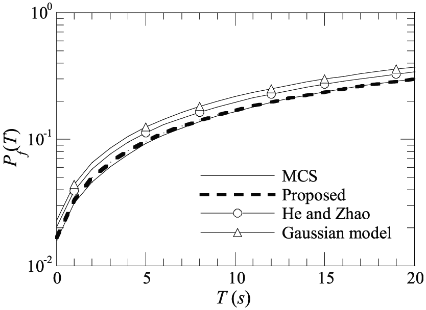
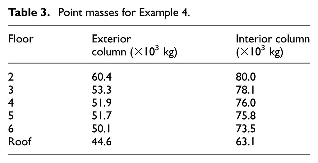
The fourth example considers a six-story moment-resisting steel frame (multi-degree-of-freedom linear system) subjected to stochastic wind load as shown in Figure 9, which has been investigated by Au and Beck (2001b) and He (2010). It is should be noted that only a continuous wind load process is considered in the example, with a relatively short time period. The member sections of the frame are given in Table 2. For each of floor, the same section is used for all girders. The structure is modeled as a two-dimensional linear frame with beam elements connecting the joints of the frame. Masses including the contributions from the dead load of the floors and the frame members are lumped at the nodes of the frame and are tabulated in Table 3. The linear dynamical system is governed by the differential equation

where
A six-story moment-resisting frame structure for Example 4.
Sections for frame members for Example 4.

Point masses for Example 4.
The undamped natural frequencies of the first six modes are computed as 0.55166, 1.56334, 2.83893, 4.48842, 6.17028, and 8.16689 Hz. Rayleigh damping is assumed for the first two modes with 5% of critical damping.
Let the wind pressure

The output non-Gaussian structural responses Ym(t), m = 1, …, 24 denotes the inter-story drift ratios of the columns at every floor. The unit impulse response function, hm(t), corresponding to Ym(t) includes the dynamics of the frame structure and the soil layers, and is obtained by deterministic dynamic analysis. The first four moments of the inter-story drift ratios of the exterior columns at every floor for the total responses, that is, the response to F(t) and for the quadratic responses, that is, the responses to α2U2(t), can be readily determined by MCS method and are listed in Table 4.
The first four moments of the inter-story drift ratios of the exterior columns at every floor for the total responses and for the quadratic responses for Example 4.
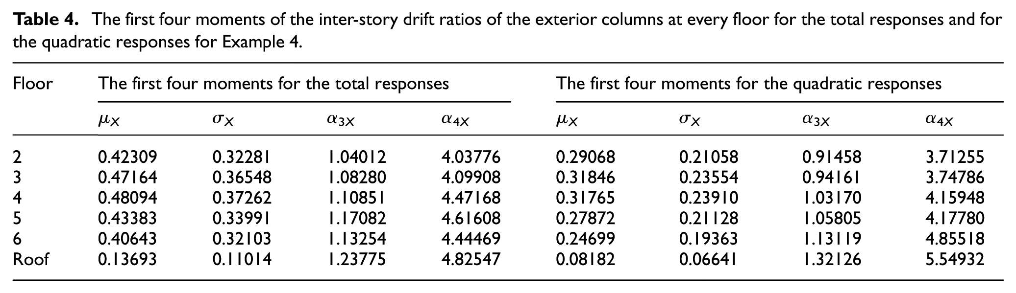
Using the first four moments of total responses as shown in Table 4 and considering the critical threshold level of x = 5σX, the variations of the first passage probability of total responses of the inter-story drift ratios with regard to excitation time T obtained using the proposed method are illustrated in Figure 10(a) to (f), together with the results obtained by assuming Gaussian model, the method proposed by He and Zhao (2007), and the MCS method (Au and Beck, 2001b; Bayer and Bucher 1999) with 100,000 samples. It can be observed that results obtained by the proposed method shows better agreements with those from MCS method than those obtained by He and Zhao method and Gaussian model, which indicates that the proposed method can be used in multi-degree-of-freedom dynamical systems for practical use.
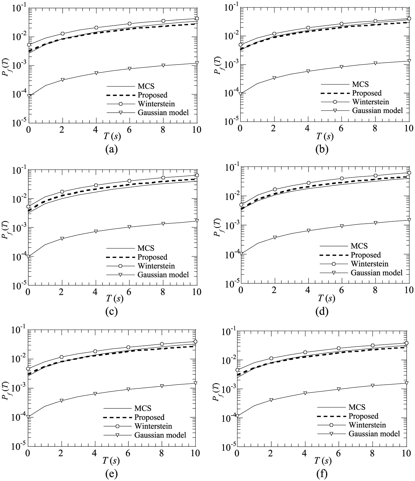
The first passage probabilities of inter-story drift ratios exceeding critical threshold level x = 5σX for the total responses in Example 4: (a) sixth story (b) fifth story, (c) fourth story, (d) third story, (e) second story, and (f) first story.
Similarly, using the first four moments of the quadratic responses in Table 4 and considering the critical threshold level of x = 5σX, the variations of the first passage probability of quadratic responses of the inter-story drift ratios with regard to excitation time T obtained using the proposed method are illustrated in Figure 11(a) to (f), together with the results obtained by assuming Gaussian model, the method proposed by He and Zhao (2007), and the MCS method (Au and Beck, 2001b; Bayer and Bucher 1999) with 100,000 samples. It can also be clearly observed that the results obtained by the proposed method are closer to MCS method than those obtained by He and Zhao method and Gaussian model throughout the entire investigation range.

The first passage probabilities of inter-story drift ratios exceeding critical threshold level x = 5σX for the quadratic responses in Example 4: (a) sixth story, (b) fifth story, (c) fourth story, (d) third story, (e) second story, and (f) first story.
Conclusion
From the investigations of this article, the following conclusions can be drawn:
A third-order polynomial transformation (fourth-moment Gaussian transformation) method is proposed for estimating the first passage probability of stationary non-Gaussian structural responses. An explicit third-order polynomial transformation is first proposed, and the inverse transformation (the equivalent Gaussian fractile) of the third-order polynomial transformation is then derived to map a non-Gaussian structural response into a standard Gaussian process.
Since the proposed explicit third-order polynomial transformation can give a good approximation for the polynomial coefficients using the first four moments, the proposed method provides more appropriate x–u transformation results compared to the current formulae.
Through numerical examples presented, it is demonstrated that for both the “softening” and “hardening” responses, the proposed method is sufficiently accurate in the calculation of first passage probabilities for stationary non-Gaussian structural responses.
The numerical results of the first passage probabilities of a moment-resisting steel frame (multi-degree-of-freedom linear dynamic system) subjected to the stochastic wind load are presented and compared with the results using other existing methods. Good agreement with MCS shows again that the proposed method is effective and accurate for practical use.
Footnotes
Appendix 1
Winterstein’s Hermite model (Winterstein, 1988) can be expressed as
in which
which
in which
For “hardening” responses, the equivalent Gaussian fractile can be taken as
Appendix 2
The mean clump size (He and Zhao, 2007) can be written as
Using the laws of conditional probability and the fact that X(t1 = x) implies with equal probability that X(t1) is either the first or the last peak in a clump; if X(t) is reasonably narrow-banded, then equation (35) can be simplified as (He, 2015)
For Gaussian result, it can be shown as
where
in which
The probability that the clump size will be exactly equal to n is
The infinite sum which appears in equation (39) must be truncated, as for large n. Equation (37) has the non-zero limit
in which u(x) is the equivalent Gaussian fractile. For SDOF system,
where N is cut-off point, which is suggested as equation (42) (He and Zhao, 2007)
Declaration of Conflicting Interests
The author(s) declared no potential conflicts of interest with respect to the research, authorship, and/or publication of this article.
Funding
The author(s) disclosed receipt of the following financial support for the research, authorship, and/or publication of this article: The research reported in this article is partially supported by the National Natural Science Foundation of China (Grant Nos 51738001, U1434204, 51422814, and 51421005), the Fundamental Research Funds for the Central Universities of Central South University (2017zzts158), and the grant of Shanghai Municipal Natural Science Foundation of China (no. 16ZR1417300). The support was gratefully acknowledged.