Decision tree–based seismic damage prediction for reinforcement concrete frame buildings considering structural micro-characteristics

Abstract

A decision tree–based seismic vulnerability method for reinforcement concrete frames is proposed. Structures with stories equal to 3, 6, 9, and 12 were considered herein and 45,360 (4 × 11,340) reinforcement concrete frame damage samples with different micro-characteristic values were simulated using the capacity spectrum method. Afterward, with the adoption of CART algorithm, a decision tree was derived to visualize the relationship between the structural characteristics and damage states according to training samples. Damage prediction can then be made for unseen structures according to their characteristic values directly using the configured decision trees. Ten training and testing sets were established randomly from the sample library and their seismic vulnerabilities under three earthquake intensity levels were assessed to verify the proposed method. The results show that the decision tree predictor is efficient for seismic vulnerability assessment of reinforcement concrete frames, and the predictor shows high prediction accuracy and stability.

Keywords

capacity spectrum method decision tree group buildings pushover analysis reinforcement concrete frame seismic vulnerability assessment

Introduction

The resilience of communities has been almost non-existent, mainly due to the high seismic vulnerability of the building stock. Recent earthquakes (e.g. China 2008, Chile 2010, and Japan 2011) have shown that the structural performance of reinforcement concrete (RC) buildings plays crucial roles in terms of earthquake losses and urban resilience (Li et al., 2008; Norio et al., 2011). Moreover, RC frame structures are commonly found in many countries. For example, they may represent approximately 75% of the building stock in Turkey, nearly 60% in Colombia, and over 30% in Greece (Yakut, 2006). Consequently, it was determined that a reliable seismic vulnerability analysis method for RC frames is of great importance.

Much research has already been performed regarding the vulnerability assessment of existing buildings. Two types of widely adopted methods were achieved: empirical and analytical. For the former, damage probability matrices (Dolce et al., 2003; Pasquale et al., 2005), vulnerability index method (Franch et al., 2008), and continuous vulnerability functions (Elnashait et al., 2004; Rossetto and Elnashai, 2005) are three main important methods based on the damage observed after earthquakes. Although these methods are clear in concept and easy to understand, they are dependent on expert judgment and opinion too. Thus, the accuracy of the results is sometime questionable.

In order to overcome the deficiency of empirical methods, analytical vulnerability assessment methods have been rapidly developed in recent years. On one hand, the damage results obtained from numerical analysis can be adopted as supplementary samples to improve the empirical methods (Barbat et al., 1996; Kappos et al., 1998). On the other hand, vulnerability assessment totally based on numerical analysis is progressively becoming a common and preferable procedure alongside the development of more advanced software tools and computational capacities. Owing to different theoretical principles, they are mainly divided into three types: collapse mechanism–based methods (Cosenza et al., 2005), capacity spectrum–based methods (Molina and Lindholm, 2005; Whitman et al., 1997), and displacement-based methods (Calvi, 1999; Crowley et al., 2004). This research tends to feature slightly more detailed and transparent vulnerability assessment algorithms with direct physical meaning, which not only allows detailed sensitivity studies to be undertake but also caters to straightforward calibration for various characteristics of building stock and hazard.

Indeed, the vulnerability analysis problem was considered in many aspects in the aforementioned studies and fruitful results were achieved. However, these researches were lacking in studies directly based on the structural micro-level. Since the seismic performance of the structure was primarily determined by the structural micro-characteristics, a much more accurate vulnerability assessment can be expected if the relationship between the structural characteristics and seismic performance is established. To this end, a decision tree algorithm (Quinlan, 1986), which is a classical machine learning model, is proposed in this article. With the adoption of the decision tree algorithm, the relationship is established by studying the training samples and visualizing tree-like decision rules. Consequently, damage prediction can be performed according to the above established decision tree for unseen structures.

The main purpose of this article is to present a micro-characteristics-based damage prediction classifier in the form of decision trees for seismic vulnerability assessment of RC buildings. To accomplish that, a total of 45,360 (3, 6, 9, 12 stories, 4 × 11,340) damage samples with different micro-characteristics were simulated by the capacity spectrum method (CSM) and the CART algorithm was then adopted to learn a damage prediction decision tree. Ten training and testing sets were established randomly from the sample library to verify the accuracy of the damage predictor. The prediction accuracy of the testing sets was evaluated by comparing with the results of the CSM. The proposed method shows great prediction performance according to the comparison results.

Sample library

Structural characteristics

The structures considered herein were 3, 6, 9, and 12 story RC frames with a regular configuration both in plan and elevation. Each building was designed according to Chinese building design codes. Here, the story number was set as the classification parameter of the structures since it is critical to the natural period and thus to their seismic vulnerability (Crowley and Bommer, 2006; Doherty et al., 2010). For the structures with the same story, five microstructural characteristics were selected as the variables due to their importance to the seismic performance of RC frames (Li et al., 2003). These characteristics include column size, column reinforcement ratio, story height, span, and depth–span ratio of beam, and their variable values are shown in Table 1. Other structural characteristics were set as constant and their values were as follows: the longitudinal size is six spans of 6 m, the transverse size is three spans, and the concrete grade of structures with different story numbers are C30, C35, C35, and C40, respectively. With the above structural characteristics, totally 45,360 RC frames were considered as the sample library for the numerical analysis.

Table 1.

Variable characteristic values of RC frames.

Structuralcharacteristics	Range	Spacing	Number
Column size (mm)
3 story	300–500	25	9
6 story	350–550
9 story	400–600
12 story	500–700
Column reinforcement ratio	1.2%–3.0%	0.2	10
Story height (m)	2.8–4.0	0.2	7
Span (m)	4.5–7.0	0.5	6
Beam section height/span	1/8, 1/10, 1/12		3
Total numberof structures	$4 \times 11, 340 = 45, 360$

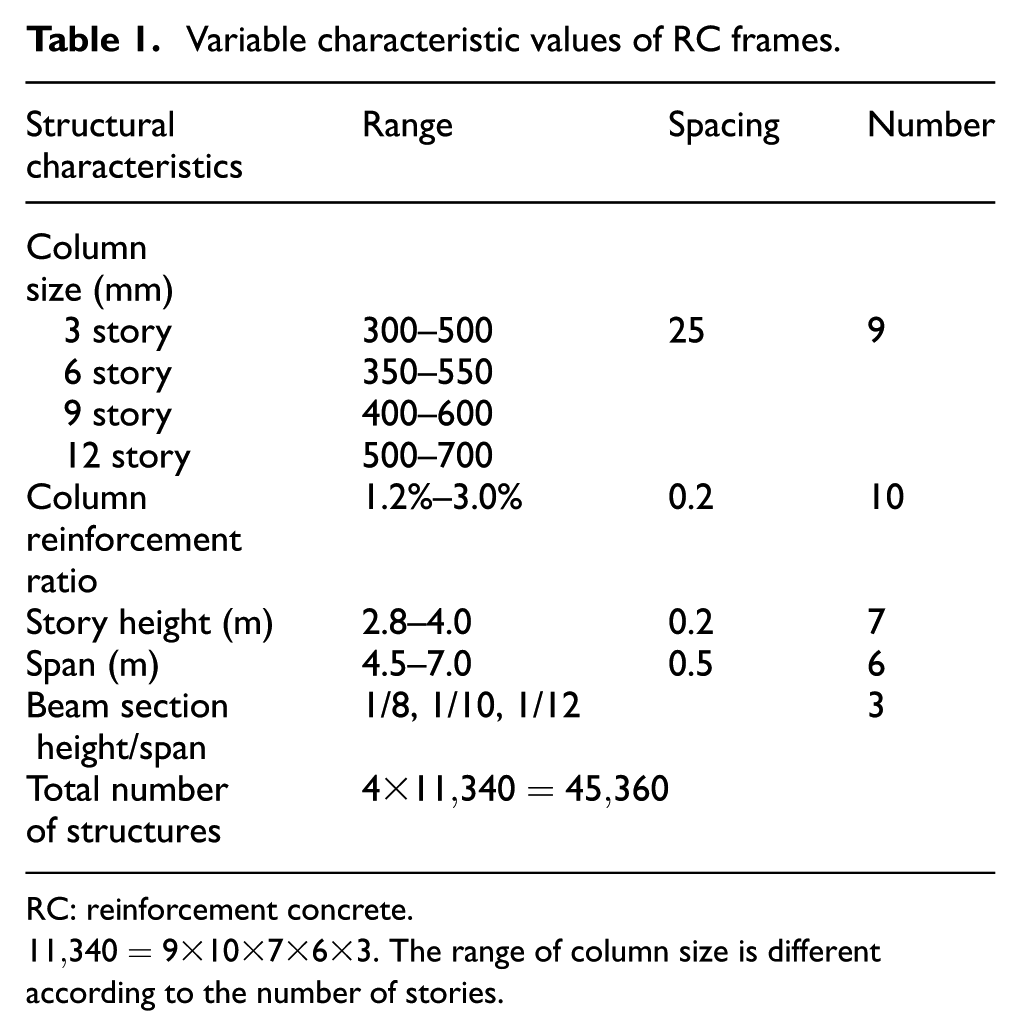
RC: reinforcement concrete.

$11, 340 = 9 \times 10 \times 7 \times 6 \times 3$ . The range of column size is different according to the number of stories.

Pushover analysis

With the adoption of the Open System for Earthquake Engineering Simulation (Mckenna and Fenves, 2013; Mazzoni et al., 2007), the pushover analysis was performed for each RC frame. Due to the symmetry of the structures, equivalent 2D plane frames were adopted for modeling simplicity. An example of such a two-dimensional (2D) frame is shown in Figure 1. In the structural modeling, (1) the dead loads, live loads, and floor dead weights were translated into equivalent distributed beam line load; (2) the constitutive relations of concrete and reinforcement materials are shown in Figure 2; (3) beams and columns were defined as fiber elements; and (4) inverted triangle loads were adopted as the lateral force.

Figure 1.

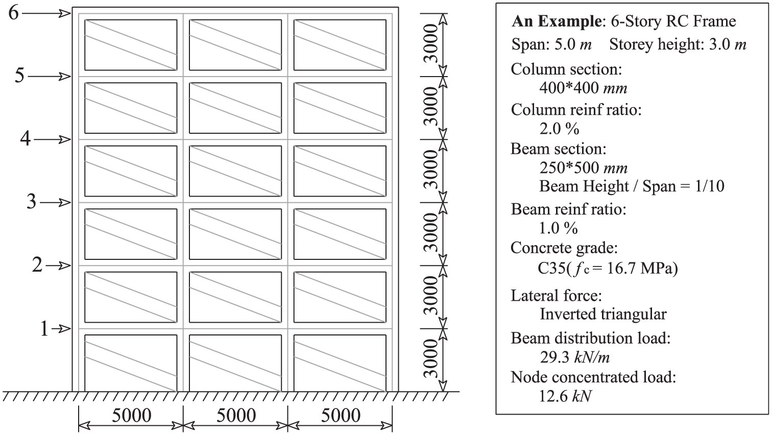
Example of an equivalent 2D frame.

Figure 2.

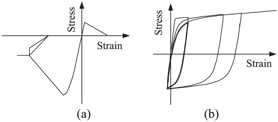
Material constitutive model: (a) concrete and (b) reinforcement.

Definition of damage states

Based on the pushover analysis, the CSM (Fajfar, 1999), one of the most important pseudo-static analysis methodologies, were performed to calculate the performance points representing the seismic demand under a certain seismic intensity. Three seismic levels equal to 0.3g, 0.45g, and 0.9g were considered in the CSM procedure to compare the damage states under different seismic intensities.

The frequently used maximum inter-story drift angle was chosen as the damage measure (DM), and the DM values of each structure were calculated by the CSM procedure corresponding to the performance point. Meanwhile, in order to represent the destruction of the structures, the relationships between the damage levels and DM values as listed in Table 2 were adopted to translate and group the DM values into damage levels from no damage to collapse. Four limit states among damage levels, DM values of which are equal to 1/450, 1/300, 1/150, and 1/50, respectively, are defined. Consequently, with the adoption of the qualitative DM, 45,360 samples with different structural characteristics and damage states were built for the following study.

Table 2.

Relationships between DM $(θ)$ and damage levels in RC frame structures.

Damage levels	No damage	Minor damage	Moderate damage	Beyond repair	Collapse
Range of DM values	1/450	1/450 ≤ θ ≤ 1/300	1/300 ≤ θ ≤ 1/150	1/150 ≤ θ ≤ 1/50	1/50 ≤ θ
Limit states		LS1	LS2	LS3	LS4

DM: damage measure; RC: reinforcement concrete.

Decision trees

Decision tree model for damage prediction

As the main novelty of this research, we use the decision tree as a classifier tool to predict the damage of RC frames under a certain seismic level according to their microstructural characteristics. Since the decision tree is a machine learning algorithm mainly used for two classification problems, four decision trees were carried out independently to judge whether a structure reaches the certain limit state LSi as listed in Table 2. In other words, the output damage prediction of the decision tree is whether a structure reaches a limit state LSi or not under a given seismic level (e.g. reaching LS1 or not under the seismic level of 0.3g). This is a supervised two-class machine learning case in which, by definition, an algorithm (classifier) should be trained by analyzing a set of classified samples called instances (e.g. structural characteristics) as input data to predict the correct class for unseen instances. Figure 3 shows an example of such a tree, which has five nodes and six leaves.

Figure 3.

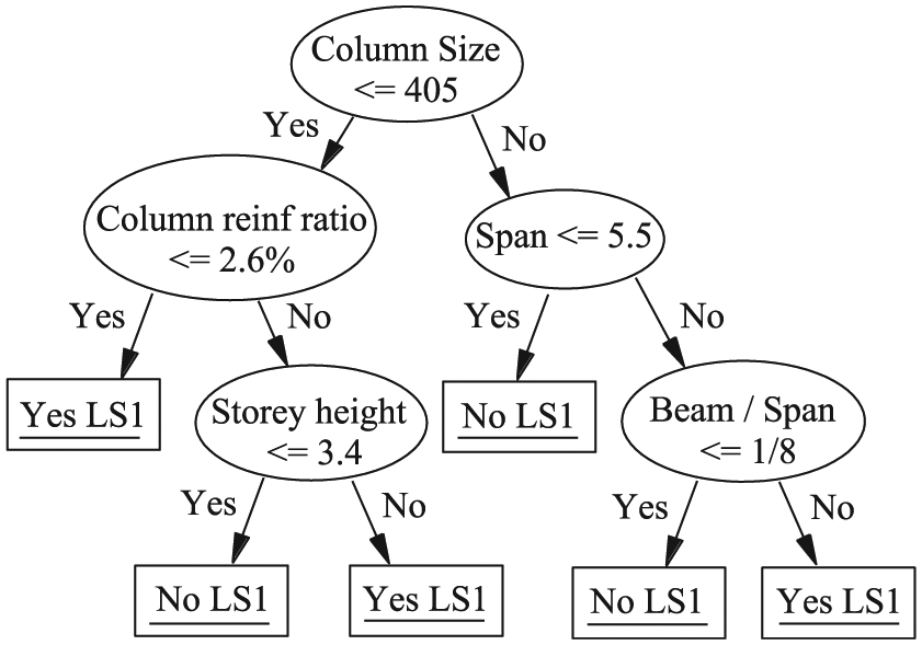
Example of a decision tree.

The example in Figure 3 shows that the decision tree is a binary tree consisting of internal nodes and leaf nodes, the former represents the decision rules and the latter represents target classification labels. The relationship between the objects of analysis that serve as input data fields and those which serve as target fields is used to create the decision rule forming the branches underneath the root node. Once the relationship is configured, one or more decision rules can then be derived that describe the relationships between inputs and targets. As we can see, the decision tree provides the means to visually examine and clearly describe the tree-like network relationship that characterizes inputs and outputs. In addition, it should be pointed out that the RC frames with different numbers of stories should refer to the different decision trees, which are trained by the instances with a same number of stories. Figure 4 illustrates the steps to follow to use decision trees for damage prediction of RC frames.

Figure 4.

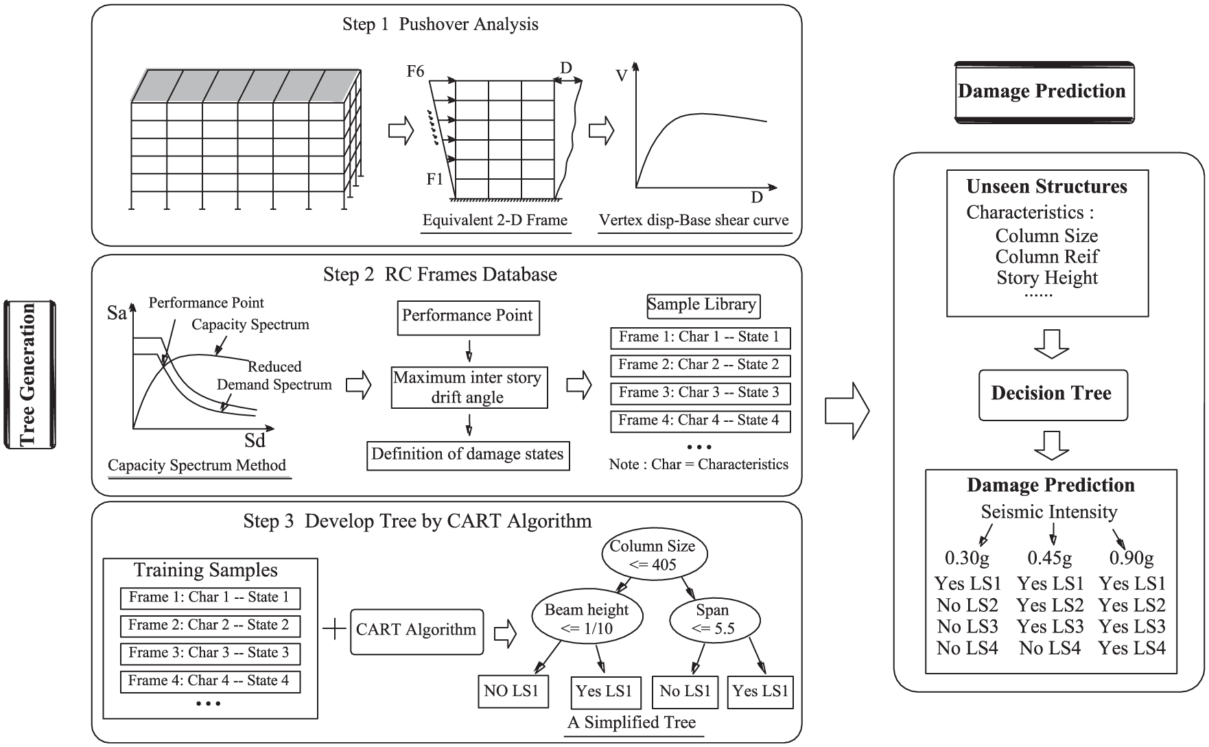
The flowchart of the proposed method.

CART algorithm

To generate the decision tree, the CART learning algorithm (Rutkowski et al., 2014), also known as a statistical classifier, was adopted. The training data in the supervised machine learning is a set S of already classified instances I₁, I₂, …, I_n. Each I_i consists of a number of features A₁, A₂, …, A_m. The training is augmented with values of C₁, C₂, …, C_n, where a certain C_i represents the class to which a certain instance I_i belongs.

The CART algorithm develops a decision tree from top to bottom according to a set of training data using the Gini-Index concept, which is the measure of uncertainty associated with the random variables. In the following part only a brief introduction of Gini-Index is presented and interested readers may refer to the literature (Strobl et al., 2007) for more information about the details of its mathematical principle.

The Gini-Index of a data set D is calculated as follows

Gini (D) = \sum_{k = 1}^{n} p_{k} (1 - p_{k}) = 1 - \sum_{k = 1}^{n} p_{k}^{2}

(1)

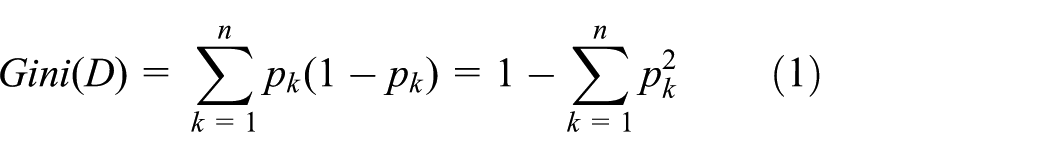
where n is the number of classes and $p_{k}$ is the frequency of the class k. The smaller the value of the Gini-Index, the smaller the uncertainty of the samples. A Gini-Index equal to zero indicates a perfectly classified set.

At each node of the tree, the CART algorithm will choose the best feature from A₁, A₂, …, A_m to divide the dataset effectively into two subsets enriched in one class or the other. The dividing efficiency is measured according to the differences in the Gini-Index resulting from a feature value for splitting the dataset. The Gini-Index for the set D over a chosen characteristic value $A_{ik}$ is calculated as follows

Gini (D, A_{ik}) = \frac{| D_{ik 1} |}{| D |} Gini (D_{ik 1}) + \frac{| D_{ik 2} |}{| D |} Gini (D_{ik 2})

(2)

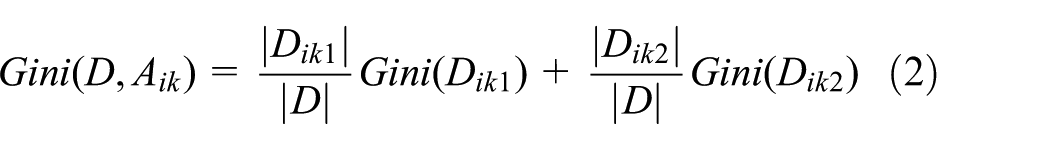
In equation (2), $A_{ik}$ is $k^{i} th$ value of characteristic $A_{i}$ , $| D_{ik 1} |$ is the number of subset 1, $| D_{ik 2} |$ is the number of subset 2, $| D |$ is the number of dataset D, $Gini (D_{ik 1})$ , and $Gini (D_{ik 2})$ is the Gini-Index calculated according to equation (1).

Based on the Gini-Index concept, features with the minimum Gini-Index are picked as the splinter node to minimize the dataset uncertainty. The data mining task of dividing the dataset to develop the damage predictor decision trees is conducted using sci-kit learn (Pedregosa et al., 2012), a powerful machine learning library based on Python.

Simulation analysis

Prediction accuracy of the decision tree

To develop and verify the decision tree, a “sufficient” number of 4000 damage samples (2000 training samples and 2000 testing samples) were selected randomly from the sample library (11,340 samples). The testing experiments were repeated for 10 times in order to make the results more reliable. As mentioned above, three seismic intensity levels of 0.3g, 0.45g, and 0.9g were considered in the article. Table 3 then lists the main damage distributions of a training set of 2000 structures under the different seismic excitations.

Table 3.

Main damage level distributions of one structural training set (2000 structures).

Seismic intensity (limit states)	0.30g (no damage–LS2)	0.45g (LS1–LS3)	0.90g(LS2–LS4)
3 story	1548	1816	1875
6 story	1927	2000	2000
9 story	1794	1971	2000
12 story	1882	1730	2000

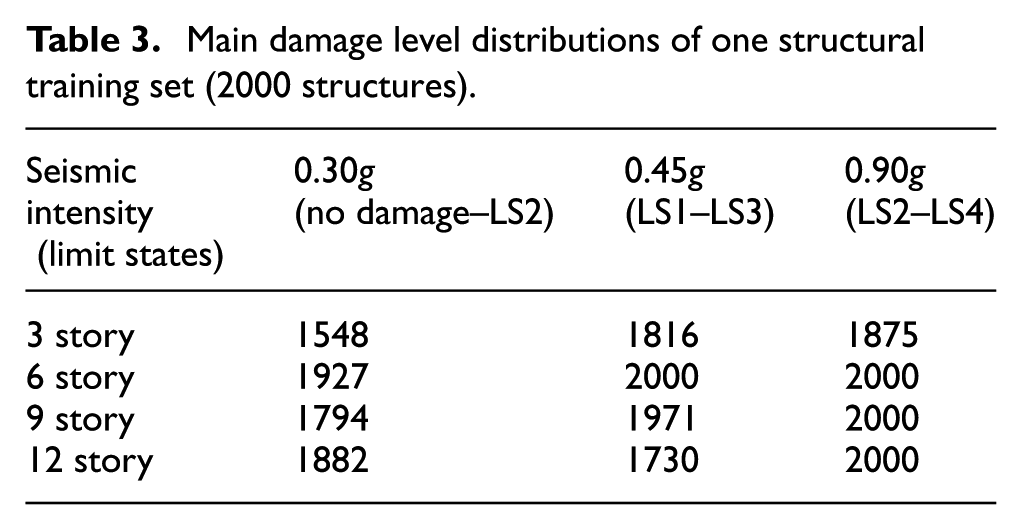
It can be found from Table 3 that for the seismic intensity level of 0.3g, the main damage distributions of 2000 randomly selected structures falls into the ranges of no damage and minor damage no matter which structural story was concerned. At the same time, for seismic intensity level of 0.45g, the ranges were minor damage and moderate damage and for seismic intensity level of 0.9g, the ranges were moderate damage and beyond repair. For this reason, only LS1, LS2, and LS3 limit states are focused on, respectively, in the following analysis according to the seismic intensity levels of 0.3g, 0.45g, and 0.9g.

Figure 5 shows the accuracy rate of the 10 testing experiments using the trained decision tree predictor when compared with the results of CSM procedure. At the same time, Table 4 lists the data of their average prediction accuracy and standard deviation. Corresponding to the seismic level of 0.3g, 0.45g, and 0.9g, the lowest average accuracies are 92.98% (six story), 90.25% (six story), 86.85% (three story), and the highest standard deviations are 0.86% (six story), 0.55% (six story), 0.93% (three story), respectively. From the above data and combining the results in Figure 5 and Table 4, we can find that the decision trees have quite high prediction accuracy no matter which seismic level is considered.

Figure 5.

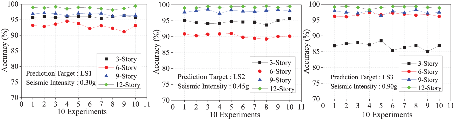
The prediction accuracy of 10 experiments.

Table 4.

The prediction accuracy of the different structure and seismic intensities.

Seismic intensity	Indicator	3 story	6 story	9 story	12 story
0.30g (LS1)	Accuracy (%)	95.92	92.98	96.71	98.80
0.30g (LS1)	Standard deviation (%)	0.25	0.86	0.35	0.32
0.45g (LS2)	Accuracy (%)	94.62	90.25	98.05	99.29
0.45g (LS2)	Standard deviation (%)	0.53	0.55	0.36	0.20
0.90g (LS3)	Accuracy (%)	86.85	96.68	97.49	99.05
0.90g (LS3)	Standard deviation (%)	0.93	0.42	0.48	0.27

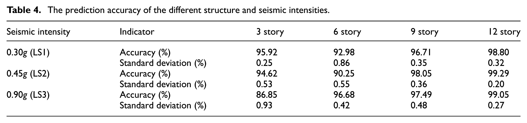
On the contrary, it should be noted that the accuracy rates have an obvious variation for RC frames with different stories. For example, the prediction accuracies under 0.45g input level are 94.62%, 90.25%, 98.05%, and 99.29%, respectively, for the 3, 6, 9, and 12 story. In order to explain this phenomenon, the following discussion is carried out furthermore.

Figures 6 to 8 show an example of the distribution of the three input characteristics (column size, reinforcement ratio of column, and depth–span ratio of beam) of the training set under the seismic input of 0.45g. In the figures, the gray represents the structures which reach the LS2, whereas the white represents the structures that do not reach the LS2.

Figure 6.

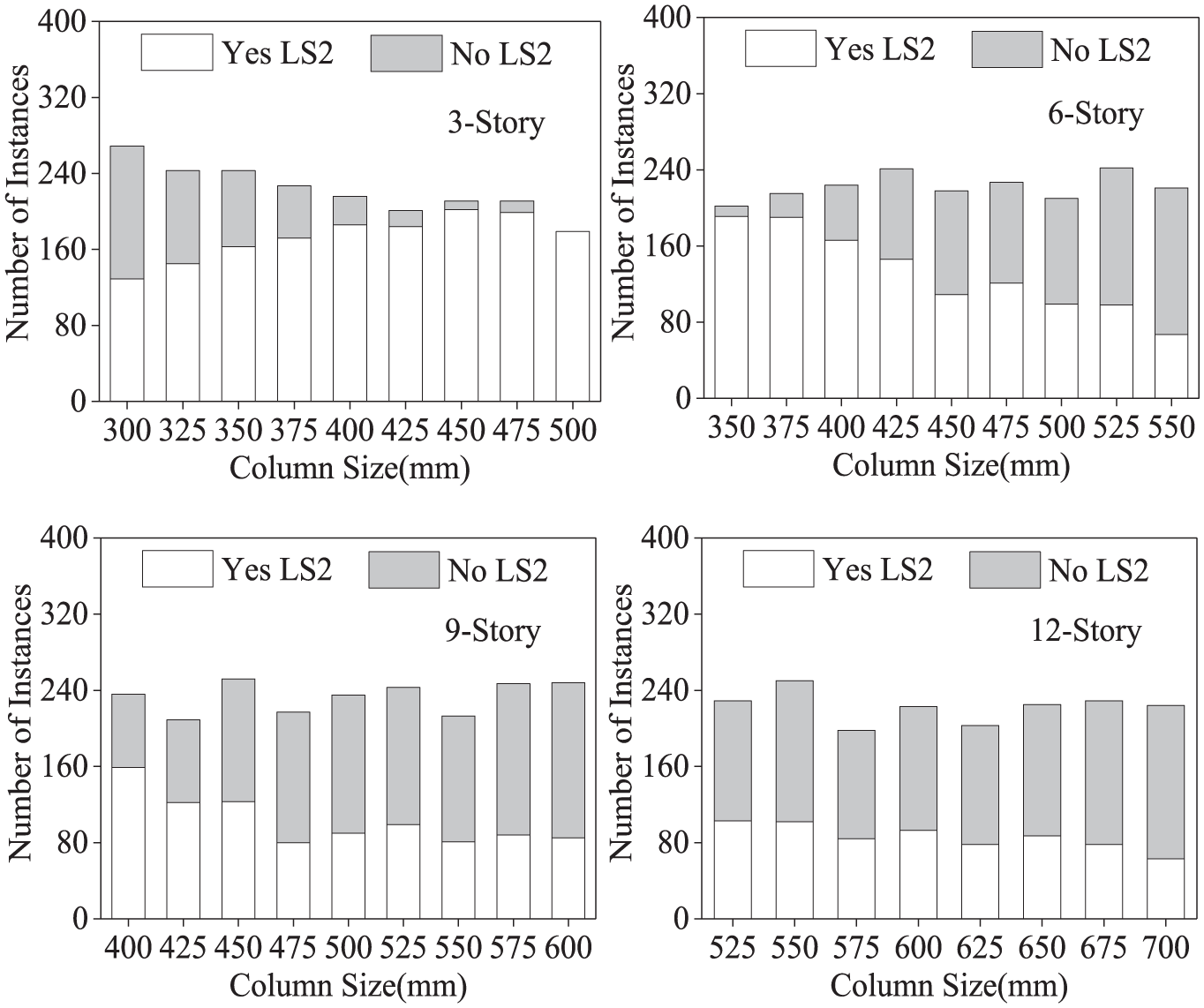
Example of a distribution of the column size for training dataset (0.45g).

Figure 7.

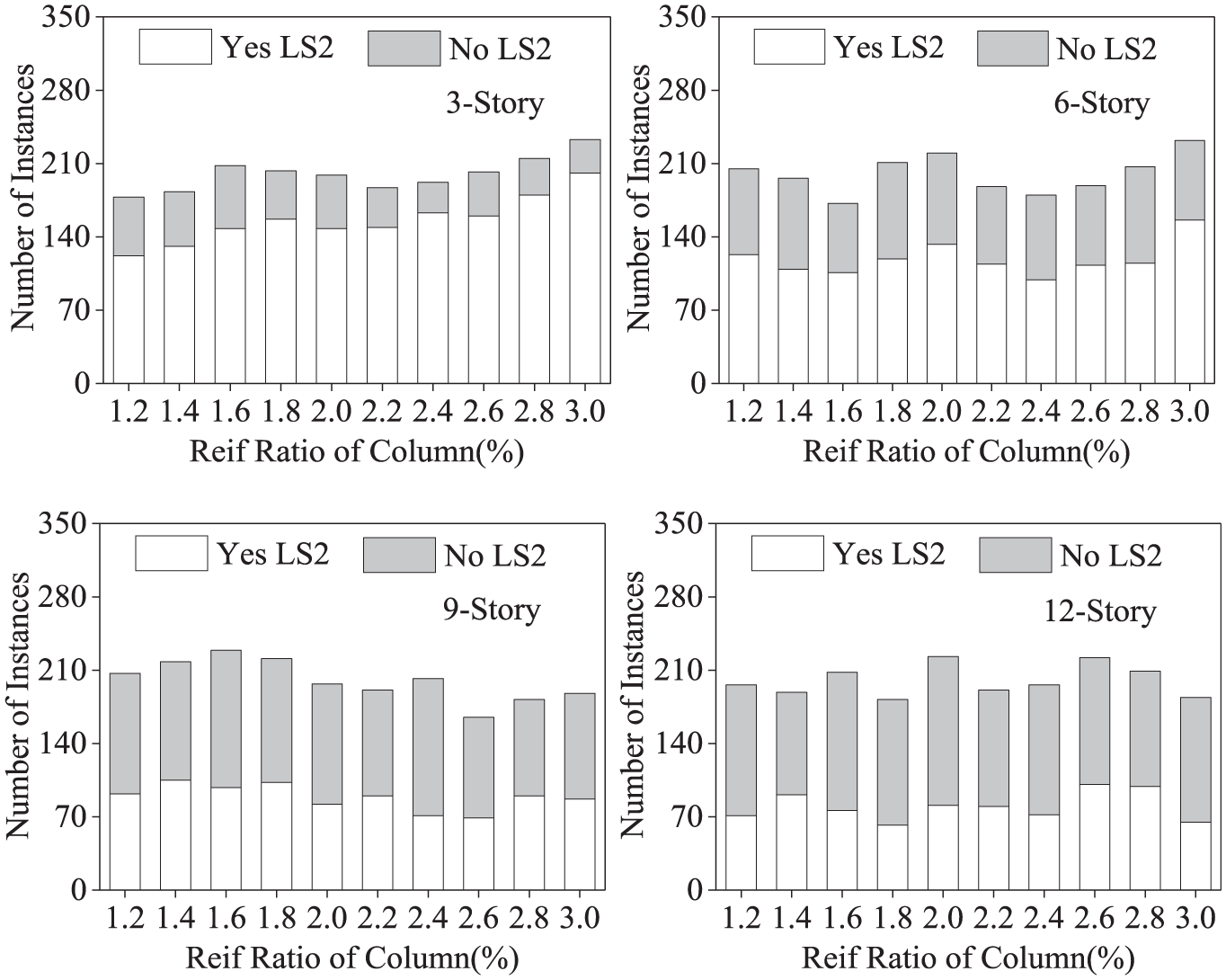
Example of a distribution of the reinforcement of the column size for training dataset (0.45g).

Figure 8.

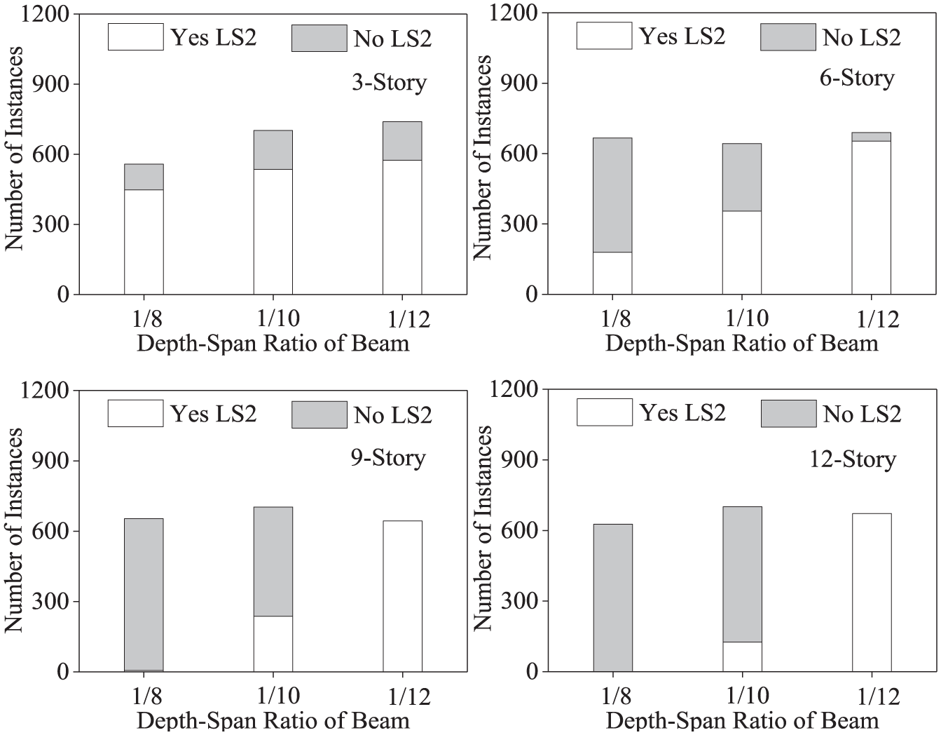
Example of a distribution of the depth–span ratio of beam for training dataset (0.45g).

Figures 6 to 8 permit the following observations: (1) the same characteristic has a quite different influence on the seismic performance for RC frames with different stories. For example, the column size has a significant influence for the 3-story and 6-story structures (Figure 6), whereas it has no notable influence for the 9-story and 12-story structures and (2) some characteristics may play a decisive role in the seismic performance of the RC frames. For example, 9-story and 12-story structures have only one damage state when the characteristic value of the depth–span ratio of beam is 1/8 or 1/12 (Figure 8), which means that a completely correct damage prediction can be made based on just one characteristic. And this result is an excellent prediction accuracy for the decision trees of 9-story and 12-story (98.05% and 99.29%).

The first observation indicates that the relationship between characteristics and seismic performance differs from structures with different stories. The latter observation indicates that a more precise decision tree will be established if the relationship between characteristics and seismic performance is simpler. And these two reasons result in the different prediction performance of the decision trees, as shown in Figure 5.

Prediction error of the decision tree

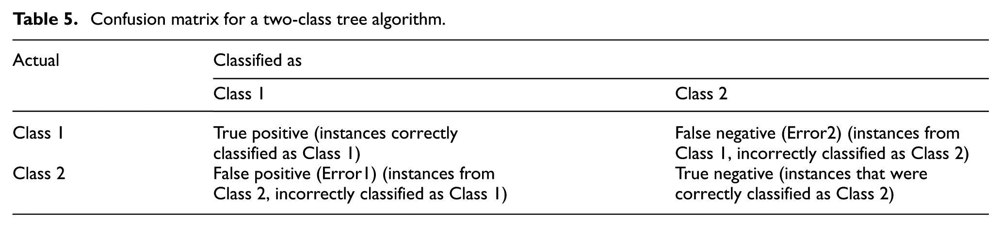
In the above discussion, we focus on the prediction accuracy and standard deviation. Actually, the prediction error is also of great importance due to the different costs of two classification error types. The error cost of misjudging an unsafe structure as a safe one is much higher than that of misjudging a robust structure as an unsafe one. For example, if the collapse-likely structure is misjudged as a safe structure, the consequence of losing the residence life will be much more serious than the reinforcement cost of a misjudged safe structure. For this reason, more attention should be paid to the former case in the practical engineering and thus it is necessary to make a further analysis on the prediction error. The confusion matrix is adopted to evaluate the prediction performance in more detail.

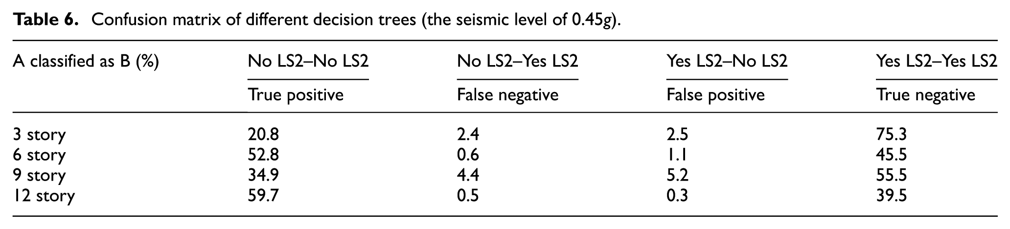
The confusion matrix is usually a 2D matrix as shown in Table 5. The rows correspond to the actual outcome, while the columns correspond to the classified outcome for the class. Elements in the matrix show how well the decision tree has correctly predicted a true outcome. Table 6 then shows the accuracy confusion matrices of the four decision trees under the seismic level of 0.45g. The following observations are permitted. (1) The sum of true positive and negative values are much bigger than that of false positive and negative values. This means the decision trees have great prediction accuracy as we have found in Table 4. (2) The prediction error of false negative which we really care about is approximately half of the total prediction error. For example, the error of false negative of the three-story decision tree is 2.5%, while the total prediction error is 4.9% (2.5% + 2.4%).

Table 5.

Confusion matrix for a two-class tree algorithm.

Actual	Classified as
Actual	Class 1	Class 2
Class 1	True positive (instances correctly classified as Class 1)	False negative (Error2) (instances from Class 1, incorrectly classified as Class 2)
Class 2	False positive (Error1) (instances from Class 2, incorrectly classified as Class 1)	True negative (instances that were correctly classified as Class 2)

Table 6.

Confusion matrix of different decision trees (the seismic level of 0.45g).

A classified as B (%)	No LS2–No LS2	No LS2–Yes LS2	Yes LS2–No LS2	Yes LS2–Yes LS2
A classified as B (%)	True positive	False negative	False positive	True negative
3 story	20.8	2.4	2.5	75.3
6 story	52.8	0.6	1.1	45.5
9 story	34.9	4.4	5.2	55.5
12 story	59.7	0.5	0.3	39.5

The influence of the number of training samples on prediction performance

In the previous research, an “enough” number of 2000 samples was selected as the training set. However, the number “2000” is subjectively determined, and a suitable number of training samples is a question worth discussing. For this reason, the results of nine different numbers of training samples equal to 10, 50, 200, 600, 1000, 1500, 2000, 3000, and 5000 were compared in the following study. Figure 9 shows the prediction accuracy trends of the nine decision trees with different training samples. In Figure 9, the scattered points represent the results of the 10 experiments, and the gray circle dots represent the average values.

Figure 9.

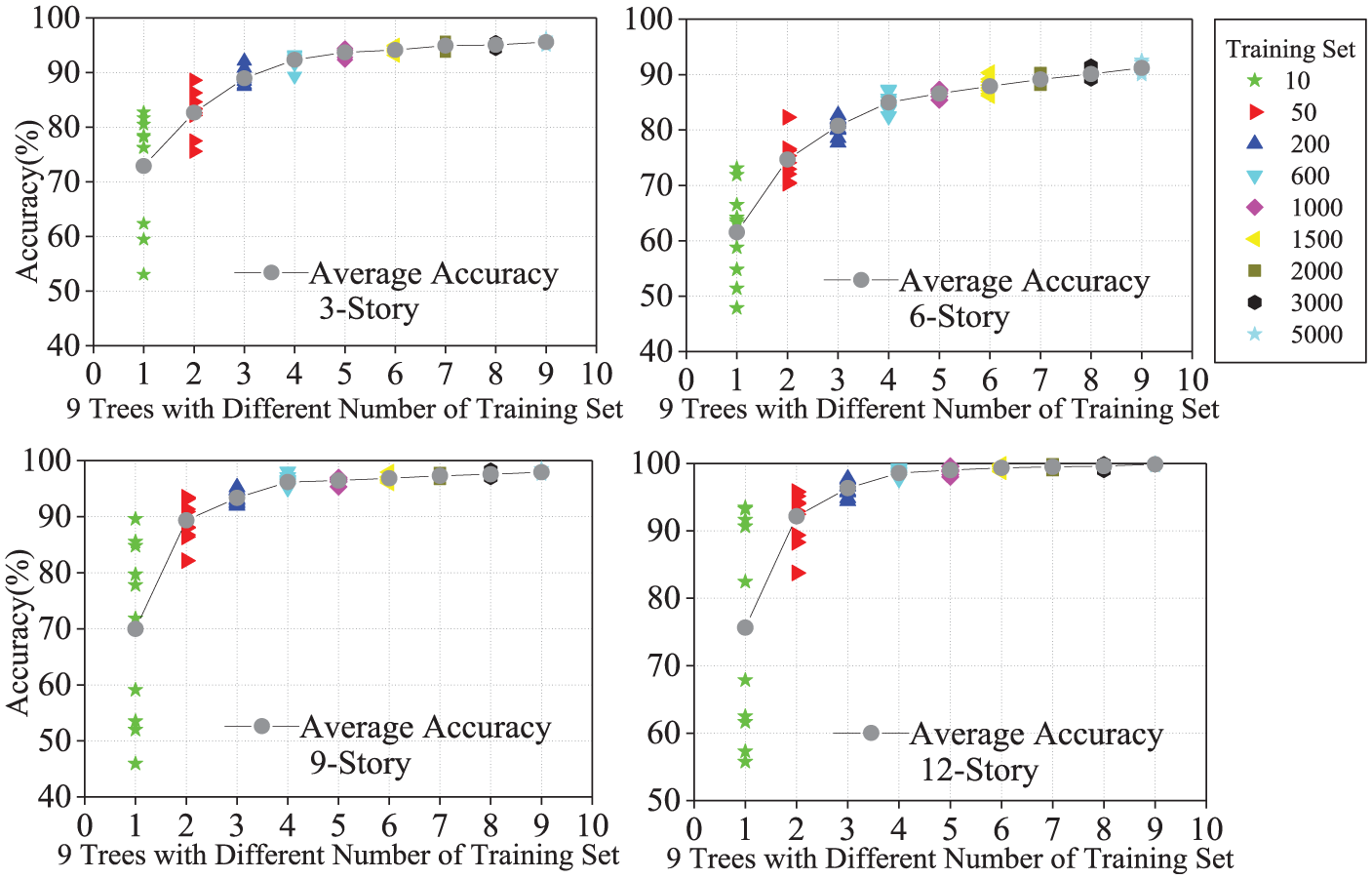
Comparison of trees of different number of training samples.

Figure 9 permits the observation that the prediction accuracy and stability are improved significantly with the increase in training samples. For example, the accuracy rate of nine-story decision tree increased from 69.22% to 97.93%. This is because the increase in the number of training samples makes the training set a better representative and thus the decision tree algorithm can learn a better overall prediction model.

At the same time, Figure 9 provides a further observation that the prediction performance is significantly improved when the number of training samples is small (10–1000), while the prediction performance is just slightly improved with a further increase in the number of the training samples (1000–5000). There are two main reasons that will account for this phenomenon: (1) 1000 samples are already enough for containing most of the characteristic values under the research environment of this article, such that the decision tree algorithm can learn a classification model with enough prediction performance and (2) there is some deviation in the numerical simulation process of the damage samples, which may bring the data a small amount of noise. In any cases, this noise will prevent the decision tree algorithm have a perfect prediction performance. And thus the prediction performance is improved slightly when the training sample number is greater than 1000.

In summary, the number of training samples has a significant impact on the prediction performance of the tree algorithm: the more the training samples, the better the prediction performance. Moreover, in the research environment of this article, 1000 training samples is enough for a precise decision tree model and is a great balance between predicting performance and calculating workload.

The influence of the validity of the training samples on prediction performance

The validity of the samples refers to whether the characteristic values of the selected training set are representative enough. Furthermore, a representative training set is uniformly distributed in characteristic values and sample categories, which means that it has great coverage of the overall database. In the previous study, 11,340 structures with characteristic values were regarded as an overall sample library for RC frames with four different numbers of stories. Generally, the smaller spacing and greater scope of the characteristic values means a better validity of the samples. To study the influence of the validity of the training samples on prediction performance, characteristic values with increased spacing as shown in Table 7 were used to reduce the data validity.

Table 7.

Characteristic values of increased spacing.

Features	Range	Spacing	Number
Column size (mm)	300–500 (3 story)	50	5
	350–550 (6 story)
	400–600 (9 story)
	500–700 (12 story)
Column reinforcement ratio	1.2%–2.8%	0.4	5
Story height (m)	2.8–4.0	0.4	4
Span (m)	4.5–6.5	1.0	3
Depth–span ratio of beam	1/8, 1/12		2
Total sample number of structures with the same story	600 $(5 \times 5 \times 4 \times 3 \times 2 = 600)$

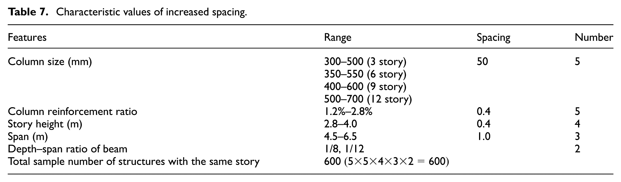
As shown in Table 7, the number of samples decreased sharply (from 11,340 to 600) due to the increase in the value interval. All these 600 samples (local data) were used as the training set to build a decision tree. Meanwhile, 600 samples were selected randomly from the original 11,340 samples as another training set to build a comparing decision tree. Ten testing experiments were carried out to check the performance of the above two decision trees; 2000 testing samples were included in each experiment, and they were all selected randomly from the original 11,340 samples.

Figure 10 shows the prediction accuracy results of 10 experiments for the aforementioned two decision trees and the following observation is permitted: the reduction in the representative of the training samples has a significant influence on the prediction accuracy, especially for the 9-story and 12-story structures (from 96.6% to 87.7% and 98.6% to 93.7%, respectively). This observation indicates that the prediction performance of the tree algorithm largely depends on the validity of the training samples. In other words, the more representative the training set, the better the prediction performance of the decision tree.

Figure 10.

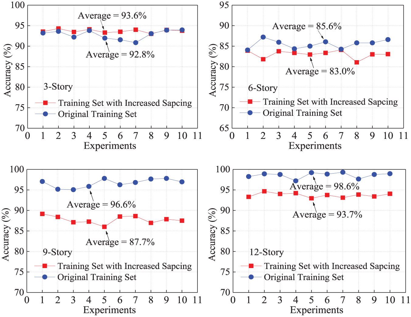
The prediction accuracy after reducing the validity of the training dataset.

The influence of the category proportion of the training samples on prediction performance

By definition, all the training samples are divided into two categories for each decision tree according to whether their damage levels reach the certain limit state LSi or not. Herein, the category proportion refers to the proportion of samples of each category to all the training samples. Since the decision tree is generated from the training samples, how the category proportion will influence the prediction performance is also an interesting question to be investigated. Following this, 12 cases of different category proportions are analyzed for comparison in this section. The seismic level is set to 0.45g and their prediction accuracy results are illustrated in Figure 11. Here, the horizontal coordinate means the category proportion of the samples that is below the limit state of LS2 and the vertical coordinate means the prediction accuracy. At the same time, Table 8 lists the data of their average prediction accuracy and standard deviation.

Figure 11.

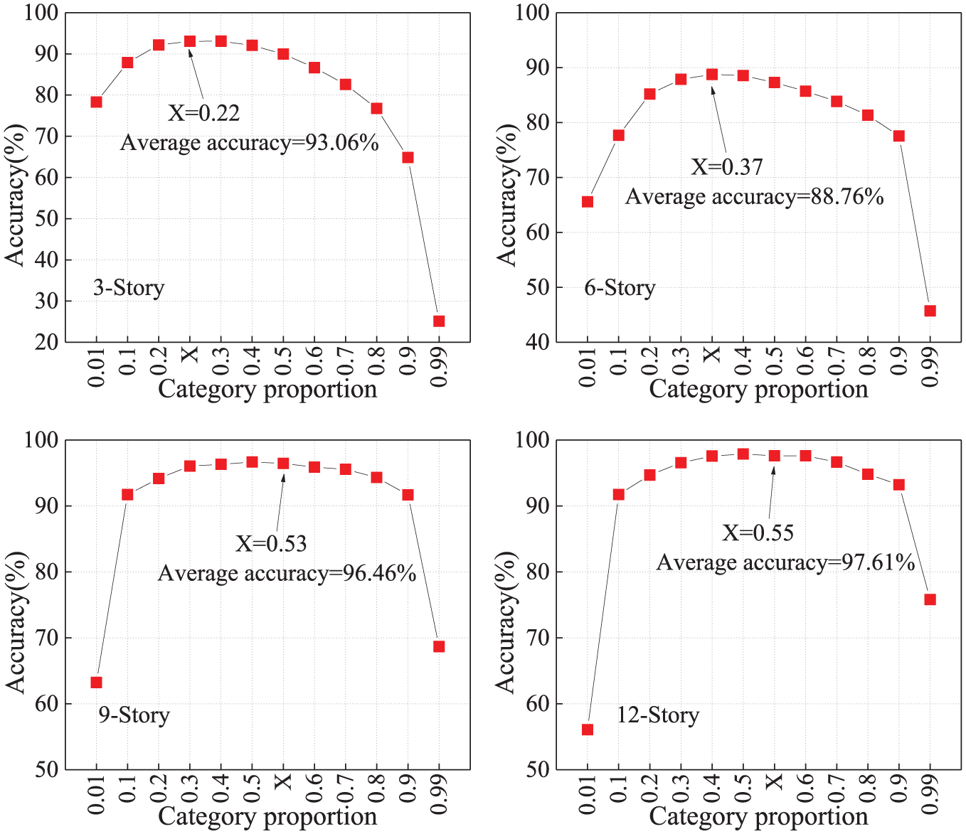
Accuracy changes of different category proportions.

Table 8.

Accuracy and standard deviation values of different category proportions.

Structures	Prediction performance	Different category predictions
Structures	Prediction performance	0.01	0.1	0.2	0.3	0.4	0.5	0.6	0.7	0.8	0.9	0.99	X
3 story	Accuracy (%)	78.31	87.87	92.17	93.07	92.05	89.95	86.65	82.57	76.76	64.85	25.12	93.06
3 story	Standarddeviation (%)	0.71	0.43	0.55	0.66	0.74	0.62	0.86	0.98	1.47	1.21	2.65	0.22
6 story	Accuracy (%)	65.56	77.66	85.18	87.87	88.55	87.28	85.69	83.84	81.34	77.54	45.72	88.76
6 story	Standard deviation (%)	1.90	1.49	0.86	0.44	0.87	0.57	0.80	0.83	0.88	0.78	4.81	0.37
9 story	Accuracy (%)	63.23	91.72	94.17	96.05	96.31	96.67	95.89	95.56	94.33	91.68	68.67	96.46
9 story	Standard deviation (%)	3.38	0.83	0.61	0.25	0.41	0.50	0.32	0.51	0.49	0.57	3.39	0.53
12 story	Accuracy (%)	56.06	91.74	94.69	96.56	97.57	97.89	97.61	96.66	94.81	93.23	75.8	97.61
12 story	Standarddeviation (%)	2.84	1.11	0.44	0.63	0.41	0.47	0.33	0.49	0.73	0.40	3.14	0.55

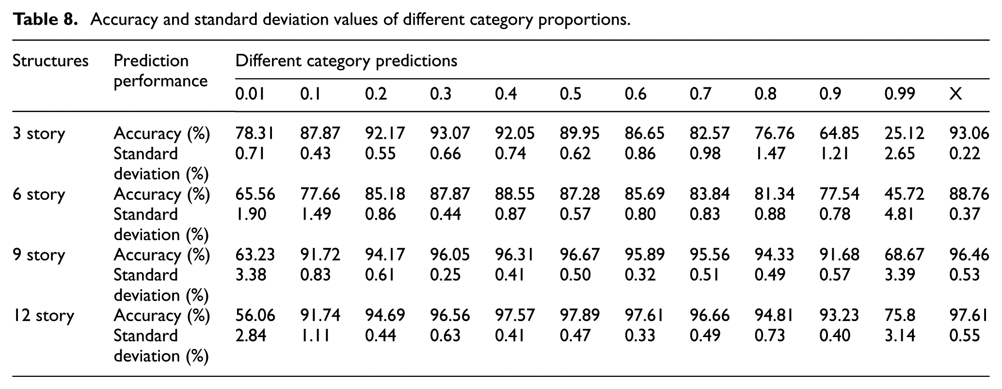
Figure 11 and Table 8 permit the following observations. (1) The prediction efficiency will not be so robust for the trained decision trees when the category proportion equals to an extreme value such as 0.01 or 0.99. For example, the prediction accuracy of six-story structures only equals to 45.72% on the proportion point of 0.99. (2) The decision trees have great prediction accuracy when the category proportions are between 0.2 and 0.8 for all structures with different stories, and 0.5 may be a good choice in the practical application. (3) As the particular case, the category proportion of the 11340 structures which is labeled as X in Figure 11 is also analyzed in this section. To be not surprised, the prediction accuracy reaches the highest point at X coordinate for all cases. That means the category proportion of training samples should be supposed to set as the same value as that of the unseen structures although it is hard to gain.

Conclusion

This article presented a quick damage prediction tool in the form of decision trees for RC frames. With the adoption of the OpenSees platform and CSM, 45360 RC frames with various structural characteristic values were simulated as the damage samples. To verify the damage prediction performance of the developed algorithm, 10 training and testing sets were selected randomly from the sample library, and the following conclusions were drawn:

The proposed decision tree method has great prediction accuracy and stability, and this provides a new feasible way for fast vulnerability assessment of RC frames.

The number of training set has great influence on the prediction performance of the trees: the more the training samples, the better the performance of the trees. The appropriate number of training samples should be the balance point between the computational workload and prediction performance.

The validity of the training samples has a significant influence on the prediction performance. In other words, a decision tree of better generalization performance will be gained based on a more effective training set.

The category proportion of the training samples is of great important. The best prediction performance will be obtained when the category proportion of the training samples is close to that of the unseen structures. The category proportion on 0.5 will be a good choice since the category proportion of unseen structures cannot be obtained in advance.

From an application point of view, there is a gap between the simulated damage samples and actual structures, and this gap will affect the prediction performance of the decision tree that is purely derived from the simulated samples. Fortunately, three structures can make the prediction model more closer to the practical application. Furthermore, refined models considering infill walls and model updating technique can be adopted to make the simulated damage samples more precise. Moreover, actual historical damage samples can be adopted as a supplementary data to modify the decision tree model. Consequently, a more robust damage prediction decision tree model can be configured and will have great application potential in the practical engineering.

Footnotes

Declaration of Conflicting Interest

The author(s) declared no potential conflicts of interest with respect to the research, authorship, and/or publication of this article.

Funding

The author(s) received no financial support for the research, authorship, and/or publication of this article.

ORCID iD

Liang Su

References

Barbat

Yepez Moya

Canas

(1996) Damage scenario simulation for seismic risk assessment in urban zones. Earthquake Spectra 12(3): 371–394.

Calvi

(1999) A displacement-based approach for vulnerability evaluation of classes of buildings. Journal of Earthquake Engineering 3(3): 411–438.

Cosenza

Manfredi

Polese

et al . (2005) A multi-level approach to the capacity assessment of existing RC buildings. Journal of Earthquake Engineering 9(1): 1–22.

Crowley

Bommer

(2006) Modelling seismic hazard in earthquake loss models with spatially distributed exposure. Bulletin of Earthquake Engineering 4(3): 249–273.

Crowley

Rui

Bommer

(2004) A probabilistic displacement-based vulnerability assessment procedure for earthquake loss estimation. Bulletin of Earthquake Engineering 2(2): 173–219.

Doherty

Griffith

Lam

et al . (2010) Displacement-based seismic analysis for out-of-plane bending of unreinforced masonry walls. Earthquake Engineering & Structural Dynamics 31(4): 833–850.

Dolce

Masi

Marino

et al . (2003) Earthquake damage scenarios of the building stock of Potenza (Southern Italy) including site effects. Bulletin of Earthquake Engineering 1(1): 115–140.

Elnashait

Borzi

Viachost

(2004) Deformation-based vulnerability functions for RC bridges. Structural Engineering & Mechanics 17(2): 215–244.

Fajfar

(1999) Capacity spectrum method based on inelastic demand spectra. Earthquake Engineering & Structural Dynamics 28(9): 979–993.

10.

Franch

KAG

Morbelli

GMG

Inostroza

MAA

et al . (2008) A seismic vulnerability index for confined masonry shear wall buildings and a relationship with the damage. Engineering Structures 30(10): 2605–2612.

11.

Kappos

Stylianidis

Pitilakis

(1998) Development of seismic risk scenarios based on a hybrid method of vulnerability assessment. Natural Hazard 17: 177–192.

12.

Xiao

Huo

(2008) Damage investigation and analysis of engineering structures in the Wenchuan earthquake. Journal of Building Structures 29(4): 10–19 (in Chinese).

13.

Liu

BGS

(2003) Performance levels and estimation indices of structures. World Earthquake Engineering 19(2): 132–137 (in Chinese).

14.

Mckenna

Fenves

(2013) Open system for earthquake engineering simulation (OpenSees). Pacific Earthquake Engineering Research Center, University of California. Available at: http://opensees.berkeley.edu/

15.

Mazzoni

Mckenna

Michael

et al . (2007) OpenSees command language manual. Available at: http://opensees.berkeley.edu/OpenSees/manuals/usermanual/OpenSeesCommandLanguageManualJune2006.pdf

16.

Molina

Lindholm

(2005) A logic tree extension of the capacity spectrum method developed to estimate seismic risk in Oslo, Norway. Journal of Earthquake Engineering 9(6): 877–897.

17.

Norio

Kajitani

et al . (2011) The 2011 eastern Japan great earthquake disaster: overview and comments. International Journal of Disaster Risk Science 2(1): 34–42.

18.

Pasquale

Orsini

Romeo

(2005) New developments in seismic risk assessment in Italy. Bulletin of Earthquake Engineering 3(1): 101–128.

19.

Pedregosa

Varoquaux

Gramfort

et al . (2012) Scikit-learn: machine learning in Python. Journal of Machine Learning Research 12(10): 2825–2830.

20.

Quinlan

(1986) Induction on decision tree. Machine Learning 1(1): 81–106.

21.

Rossetto

Elnashai

(2005) A new analytical procedure for the derivation of displacement-based vulnerability curves for populations of RC structures. Engineering Structures 27(3): 397–409.

22.

Rutkowski

Jaworski

Pietruczuk

et al . (2014) The CART decision tree for mining data streams. Information Sciences 266(5): 1–15.

23.

Strobl

Boulesteixb

Augustina

(2007) Unbiased split selection for classification trees based on the Gini Index. Computational Statistics & Data Analysis 52(1): 483–501.

24.

Whitman

Anagos

Kircher

et al . (1997) Development of national earthquake loss estimate methodology. Earthquake Spectra 13(4): 643–661.

25.

Yakut

(2006) Reinforced concrete frame construction (World Housing Encyclopedia–Summary publication). Available at: http://www.world-housing.net/wp-content/uploads/2011/06/RC-Frame_Yakut.pdf