Method to test the durability of fiber-reinforced polymers based on elastic modulus

Abstract

The performance degradation of fiber-reinforced polymer is often assessed based on the ultimate strength obtained during a destructive test. This method has the advantages of simple operation, clear internal mechanism, and noticeable data variation. However, because fiber-reinforced polymers are composed of high molecular compounds, their properties are influenced by several factors, such as the manufacturing process and composition ratio. Without a unified benchmark, it is difficult to unify destructive test data obtained by different researchers and organizations. In this study, a new test method named SNFT (Same Non-failure FRP Test) is proposed for assessing the durability of fiber-reinforced polymers. SNFT is a testing method in which the same specimen can be repeatedly tested at different aging periods. The rationality of the SNFT method is analyzed using the displacement compatibility between the degraded zone and the undegraded zone. The conversion principle based on the degraded degree between the destructive test and the SNFT method is deduced by calculation. An experimental test was designed to investigate the test conditions and control parameters of the SNFT method. SNFT and synchronous destructive tests on glass fiber–reinforced plastic were carried out under the conditions of wet heat and alkali solution, and the theoretical results were compared and verified with data in the literature. The results show that compared with the traditional durability destructive test method, the SNFT method shows more consistent data and less data fluctuation and incurs a lower test cost. The elastic modulus, adopted as the durability benchmark, can be similar to the test results of traditional destructive test methods and could be transformed based on the transformation relationship proposed in this article. The degradation of fiber-reinforced polymer in different environments is characterized by the variation in elastic modulus measured using the SNFT method. This study provides a theoretical basis for establishing a unified benchmark of durability tests and data and supports the quantitative design of durability.

Keywords

durability elastic modulus fiber-reinforced polymer SNFT (Same Non-failure FRP Test)

Introduction

Fiber-reinforced polymers (FRPs) have several advantages, such as high strength, lightweight, and good durability. They are widely used in several fields and applications, such as aerospace, building structures, marine engineering, nuclear power engineering, and water conservancy engineering (Pan and Xian, 2019). With the broader application of FRP, the environment is getting worse. Although FRPs exhibit good durability, they still experience different degrees of degradation under harsh environmental conditions, which affects the performance of FRP (Karbhari, 2009; Pan et al., 2019; Prabhakar et al., 2019; Yang, 2010).

In recent years, many scholars have carried out experimental studies on the durability of FRP (He et al., 2020; Al-Safy et al., 2014; Dong et al., 2018). The relationships between the ultimate strength, elastic modulus, elongation, and degradation time of FRPs under different environmental conditions have been studied (Liang et al., 2019; Yang et al., 2018; Yu, 2018). The durability of FRP has been measured by applying the reduction of ultimate strength, and the degradation model and degradation law of FRP sheets in different environments have been established (Hedayat and Baniasadizade, 2015; Xu, 2013). However, all these tests applied destructive test methods. Physical and mechanical parameters, such as the ultimate strength, elastic modulus, and elongation, were obtained from the stress–strain relationship through the ultimate tensile test before and after degraded aging (Frigione and Lettieri., 2018; Li et al., 2009; Ouyang and Wan., 2010). This method is useful in the study of materials with stable properties, such as steel, and can compensate for the lack of data by increasing the number of tests and taking the average of multiple test results. However, the application of destructive test methods significantly increases the number of test samples and the complexity of data processing (D’Antino and Pisani, 2018; Kim et al., 2008). Due to the robust design capability of FRPs, the ultimate strength, elastic modulus, and other material properties are influenced by human factors, such as specimen fabrication and processing. The degradation of material properties before and after degradation is influenced by the variations in the mechanical properties, which is unfavorable in the analysis of the degradation of FRP durability. Therefore, highly accurate degradation data cannot be obtained (Ceroni et al., 2006; Chen et al., 2007).

Elastic modulus is an essential property of engineering materials. Elastic modulus can measure the ability of materials to resist elastic deformation macroscopically, and it can indicate the bonding strength of micro-particles in the material microscopically. Therefore, the change in elastic modulus reflects the change in material interior, such as the change in chemical composition and the appearance of microcracks. The degradation of materials is an external manifestation caused by changes in the chemical composition and microstructure of materials; hence, the elastic modulus could be used as a mechanical index for measuring the degree of change. FRP is composed of a kind of high molecular compound, characterized by lightweight and high strength. During the design process of an FRP structure, the ultimate strength can easily achieve the standard. However, in reaching the ultimate strength, the sectional area of the member becomes small and the stiffness of the structure is often insufficient because of the FRP’s high ultimate strength. In most cases, therefore, the design of FRP structures is controlled by the stiffness. In most FRP structural design cases, the elastic modulus of FRP should be considered more. When the FRP structure is degraded by the environment, the change in elastic modulus will more likely affect the performance of the FRP structure. Thus, for an FRP structure, the elastic modulus is suitable for determining the durability index to indicate the durability level.

Principle of SNFT (a testing method in which the same specimen can be repeatedly tested at different aging periods)

After an FRP material becomes degraded in time t, its elastic modulus and ultimate strength will be damaged to some extent. Based on the change in the material section during the FRP degradation process, the degradation law of mechanical properties is deduced. In this study, the following rational assumptions are made to simplify the calculation and facilitate the derivation:

In the vertical direction of the fibers, the fibers are evenly distributed across the vertical section of the fibers.

The FRP degraded process takes place gradually from the surface to the interior.

The degraded part of the material has different properties from that of the FRP material. In the study area, the interfacial shedding of the fiber surface and structural micro-damage are reflected by the change in the mechanical properties of the studied area. Such changes in mechanical properties include the shedding of the fiber interface and the change in the properties of resin materials and fiber materials.

The FRP degradation model is a one-dimensional degradation model, which considers only degradation in the depth direction.

Stress concentration is ignored due to the degraded notch.

The elastic modulus and ultimate strength of materials in the degraded zone decrease to a certain extent, compared with those in the undegraded zone. The material properties are shown in Figure 1.

Figure 1.

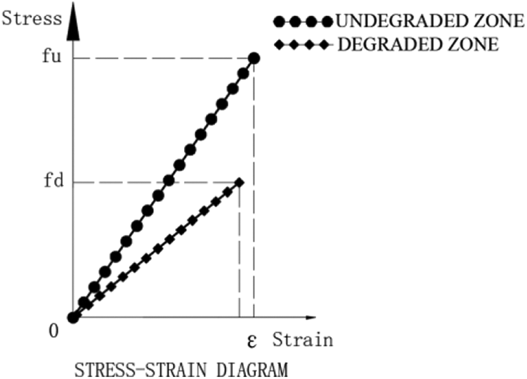
Stress–strain diagram.

Based on the degrading process of FRP, the change in cross-section during the degraded process is shown in Figure 2.

Figure 2.

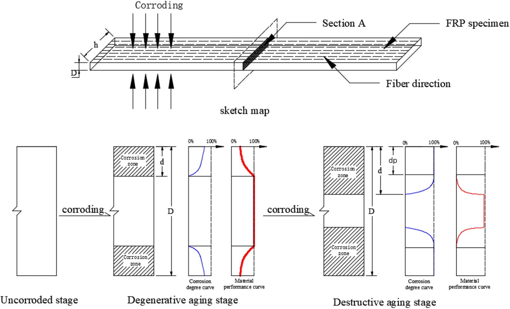
Section A change diagram during degradation.

As shown in Figure 2, the degradation of FRP can be categorized into two stages, namely the degenerative stage and destructive stage. The specimen thickness is D and the degraded depth is d during the degenerative stage. After time t, the material performance degrades, but the material can still bear part of the load. With the deepening of the depth, the degraded degree gradually weakens, and the material performance gradually degrades.

During the destructive stage, the material property degrades to zero, and the materials in the degraded areas can no longer resist the external load. Here, the material is completely degraded, and the depth in the area where the material property degrades to zero is called the destructive degraded depth dp. Due to the good durability of FRP, it takes a long time for the FRP to be completely degraded. The degradation during the laboratory rapid test generally occurs during the degenerative aging stage. In this study, the degradation during the degenerative aging stage is assessed and the principle of the SNFT (Same Non-failure FRP Test) method is analyzed to determine the relationship of the elastic modulus drop ratio and the ultimate strength drop ratio with the degraded depth.

The distribution of mechanical properties in the degraded zone is simplified to a rectangular distribution to facilitate the theoretical derivation and calculation, as shown in Figure 3. Figure 3 shows the simplified process of material property distribution of Section A of Figure 2.

Figure 3.

Material distribution model diagram of Section A.

After degradation occurs, FRP is divided into two parts: degraded zone and undegraded zone. The material in the undegraded zone is a uniform material, whose elastic modulus is E and ultimate strength is F. The material in the degraded zone is a material with uniform distribution of material properties. The average value is used to calculate the material properties, E ₁ and f ₁, as follows

f_{1} = α f; E_{1} = β E

The thickness of the specimen is D. After time t, the thickness of the undegraded zone of the specimen is d. The material properties before and after degradation are shown in Table 1.

Table 1.

Material attribute table before and after degradation.

Region	Elastic modulus	Ultimate strength
Undegraded zone	E	f
Degraded zone	E ₁	f ₁
Combination	$\bar{E}$	$\bar{f}$

In the case of tension at both ends, based on the displacement coordination condition, set the overall strain of the final sheet as $ε$ and the external force acting on F

ε E_{1} \times d + ε E \times (D - d) = F

\bar{E} = \frac{F}{ε D}

Combining equations (1) to (3), the following is obtained

\bar{E} = E (1 - (1 - β) \frac{d}{D})

The ultimate strain is assumed to be $ε_{u}$

f_{1} \times d + ε_{u} E \times (D - d) = F

The yield strength of the degraded area is lower than the ultimate strength of the undegraded area. Therefore, the ultimate strain during the failure stage is the strain in the undegraded area

ε_{u} = \frac{f}{E}

Substituting equation (6) into equation (5)

f_{1} \times d + f \times (D - d) = F

Substituting equation (7) into equation (1) gives the ultimate strength of the entire member

\bar{f} = \frac{F}{D} = (1 - (1 - α) \frac{d}{D}) f

Combining equations (4) and (8), the following is obtained

\frac{\bar{f}}{f} = 1 - (1 - α) \frac{1 - \bar{E} / E}{1 - β}

Here, $\bar{f} / f$ is the residual strength rate of the FRP sheet, $\bar{E} / E$ is the elastic modulus residual rate of the FRP sheet, α is the proportion of the ultimate strength of the degraded zone, and $β$ is the proportion of the elastic modulus of the degraded zone.

$γ$ , $f_{r}, and E_{r}$ are given as follows

γ = \frac{1 - α}{1 - β}

f_{r} = \frac{\bar{f}}{f}

E_{r} = \frac{\bar{E}}{E}

In the equation above, f_r is the residual strength rate, E_r is the elastic modulus residual rate, and $γ$ is the conversion coefficient of SNFT to failure test. The value of $γ$ is related to the type of FRP, environmental conditions, and manufacturing process and formula of FRP

f_{r} = γ E_{r} + 1 - γ

As shown in equation (13), the decrease in the ratio of elastic modulus before and after FRP degradation is proportional to the decrease in the ratio of ultimate strength. With the decrease in elastic modulus, the ultimate strength also decreases. Equation (13) can link the elastic modulus measured by the SNFT method with the ultimate strength measured by the destructive test and can transform each other. The conversion is related to the FRP and the external environment.

SNFT method

SNFT, based on the elastic modulus, can measure the deterioration of material performance with a slight effect on the material. SNFT has the advantages of low test cost and high data reliability and can be used in FRP durability tests. Regardless of the degradation degree, the stress and strain of the FRP are proportional to each other before failure occurs. This proportionality means that the elastic modulus remains unchanged before failure takes place. In theory, the elastic modulus can be measured without affecting the performance of specimens. In each test, ideal results can be obtained by stretching the specimens to a specific load. Therefore, the elastic modulus of the same specimen at different aging periods can be measured without destroying the specimen, and the curve of elastic modulus with respect to time can be obtained (Prabhakar et al., 2019).

According to the principle of SNFT, the relationship between elastic modulus and ultimate strength is linear. The coefficient of linear relationship is related to the degraded depth, and then, the degraded depth can be obtained from the elastic modulus and ultimate strength, which can guide the quantitative design of durable FRPs in the future.

Therefore, SNFT of FRP sheet can be applied using elastic modulus as the index. The test can be classified into two parts: test parameter determination experiment and SNFT durability.

Experiment 1

Experimental design

The purpose of Experiment 1 is to study the effects of different loading modes and levels on the SNFT results, determine the optimal loading mode and loading level, and ensure that loading has the least impact on the results.

The test procedures are given as follows:

The specimens are marked and numbered.

The loading control conditions and loading levels are determined.

The specimen is stretched to the preset loading level, and the stress and strain data are recorded.

From the stress–strain curve, the data are linearly fitted, and the slope of the fitting line is the elastic modulus.

The data fluctuation of different loading modes are compared and analyzed, and the loading conditions and loading point of the load are determined.

The tensile test is based on Chinese standards, Test Method for Tensile Properties of Orientation Fiber Reinforced Polymer Matrix Composite Material (GB/T 3354:2014, 2014), TM4504. A microcomputer-controlled electronic universal testing machine was used, and loading was applied at a loading rate of 2 mm/min. Strain was measured using an extensometer with a range of 10 mm.

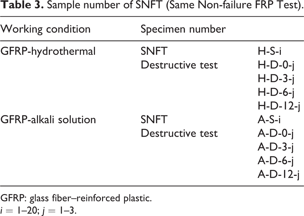
Two groups of tests were designed: force-controlled group and displacement-controlled group. Five loading levels were set for each group of specimens. There were eight specimens in each group, and each specimen was measured thrice. The number of specimens is given in Table 2.

Table 2.

Number of test specimens for parameter determination.

Loading mode	Loading level	Specimen number
Force controlled	10% f_u	F-10-i
	20% f_u	F-20-i
	30% f_u	F-30-i
	40% f_u	F-40-i
	50% f_u	F-50-i
Displacement loading controlled	10% $ε_{u}$	D-10-i
	20% $ε_{u}$	D-20-i
	30% $ε_{u}$	D-30-i
	40% $ε_{u}$	D-40-i
	50% $ε_{u}$	D-50-i

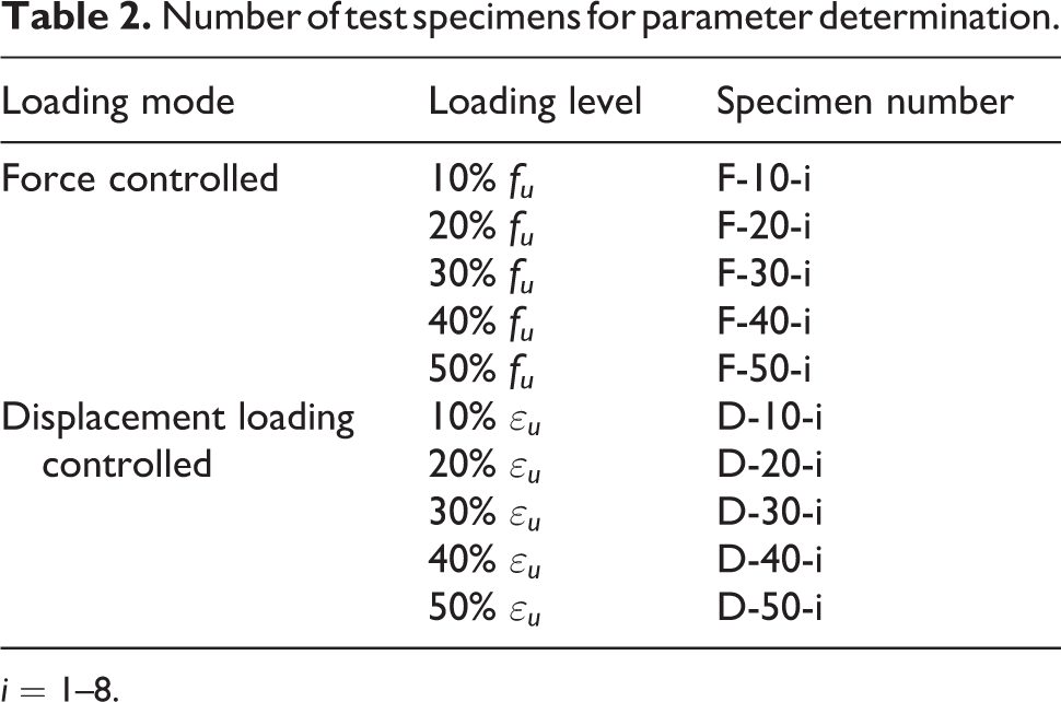
i = 1–8.

Test results

Tensile tests of different load/displacement grades were performed for each group of specimens, which were 10%, 20%, 30%, 40%, and 50%. The elastic modulus was measured, and its numerical fluctuations were compared and analyzed. The experimental results are presented in Appendix 1.

Data variance of different loading levels is shown in Figure 4. The force-control mode has a smaller data variance than the displacement-control mode. When the loading level is low, the data collection point is insufficient, and the data fluctuation is high. When the loading level is high, the internal damage of the specimen is caused by the large external load, and the measured elastic modulus fluctuation is high. By considering both factors, the force-control mode is adopted, and the loading point is at 30% ultimate load.

Figure 4.

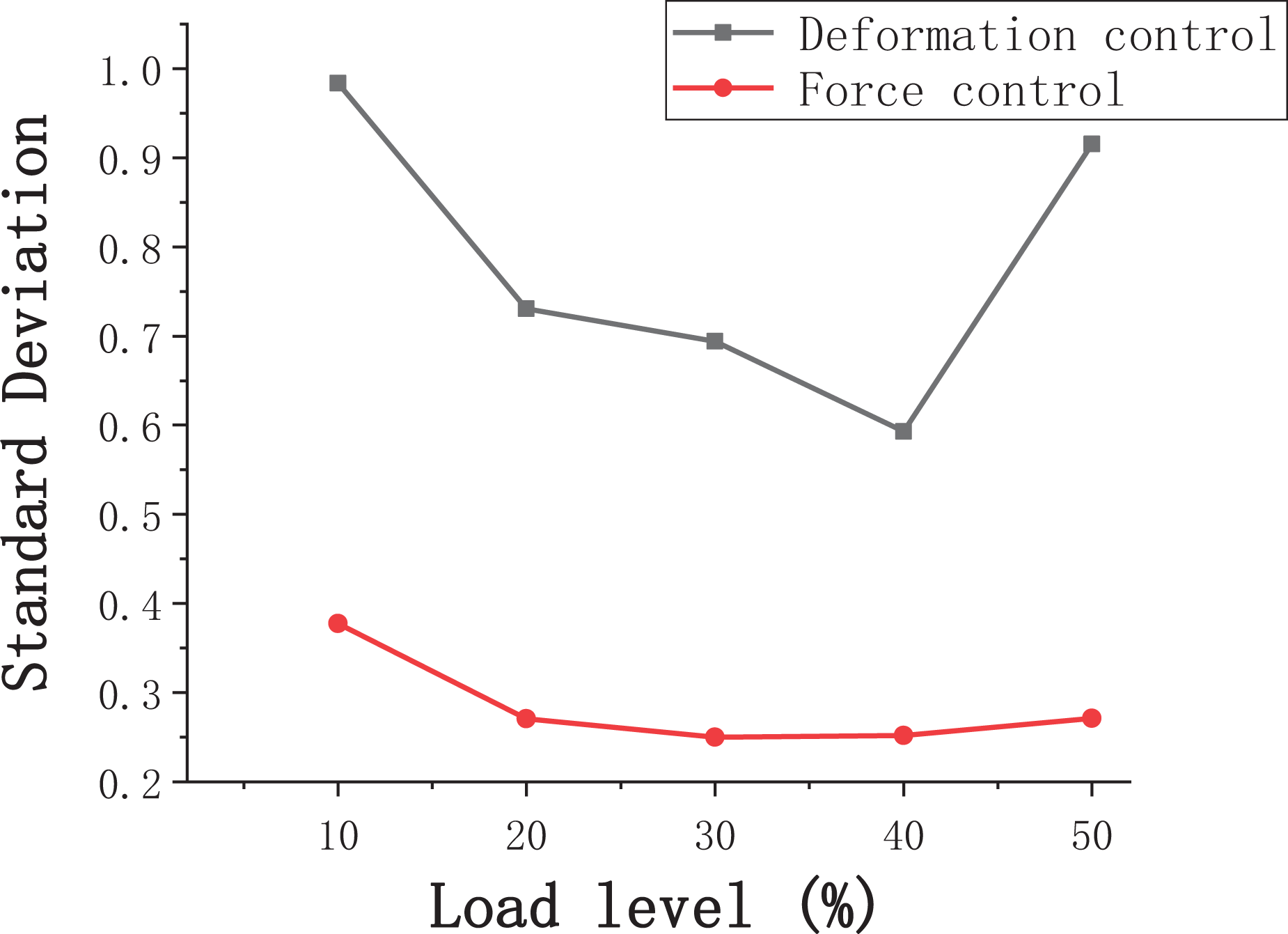
Variance diagram of data with different loading levels.

Experiment 2

Experimental design

In Experiment 2, two groups of experiments were set up: alkali solution degradation test and hydrothermal environment degradation test of glass fiber–reinforced plastic (GFRP). The destructive test and SNFT test were conducted for the two test groups. The purpose of the tests is to verify the feasibility of the SNFT test method and to determine the relationship between the results of the SNFT and destructive tests.

The test procedures are given as follows:

The specimens are marked and numbered.

Durability aging operation was performed on the specimens.

The specimens were stretched to the loading point, the stress–strain curve was plotted, the elastic modulus was calculated, and the above operations were repeated several times to obtain the respective average values.

The tensioned specimens were further degraded.

Operations 2 and 4 are repeated until the test is completed.

The tensile test of the specimen is consistent with the parameter determination test in section “Experimental design.” The load is slowly unloaded after the test is stretched to the loading point determined in Experiment 1.

In the experiment, the SNFT consisted of 20 specimens, each of which was tested thrice. The destructive test was categorized into four groups according to different degraded times, and there were three specimens in each group. The specimens were manufactured according to relevant specifications (ACI 440.3R:2004, 2004). The hydrothermal environment was simulated using an SH-221 hydrothermal environment test box. The specific environmental factors were as follows: Temperature was 60°C ± 2°C, and relative humidity was 93% ± 3%. NaOH solution with 3% mass fraction was used in the alkali solution. The sample number table is shown in Table 3.

Table 3.

Sample number of SNFT (Same Non-failure FRP Test).

Working condition	Specimen number
GFRP-hydrothermal	SNFT	H-S-i
	Destructive test	H-D-0-j
		H-D-3-j
		H-D-6-j
		H-D-12-j
GFRP-alkali solution	SNFT	A-S-i
	Destructive test	A-D-0-j
		A-D-3-j
		A-D-6-j
		A-D-12-j

GFRP: glass fiber–reinforced plastic.

i = 1–20; j = 1–3.

Test results

GFRP-hydrothermal

Appendix 2 presents the destructive test data of GFRP in the hydrothermal environment, and Appendix 3 shows the SNFT test data of GFRP in the hydrothermal environment. It can be seen that there are 28 specimens in the destructive test. Without considering the elongation data, 56 specimens were measured. The SNFT consisted of 20 specimens from 240 measured specimens. The SNFT test is six times more efficient than destructive tests.

Figure 5 shows the relationship between the elastic modulus drop ratio of GFRP-SNFT and time in the hydrothermal environment. Figure 5 includes the elastic modulus of each specimen at different aging times and the average value of all specimens. The curves of the different specimens form the blue part of the envelope, whereas the width of the envelope reflects the degree of data concentration. The width of the envelope diagram is smaller, and the data are more concentrated. The curves of different specimens exhibit the same trend. From the average elastic modulus of all the specimens, it can be seen that with the increase in degraded time, the elastic modulus decreases gradually. The decrease is faster during the early stage, and the degraded rate slows down in the later stage.

Figure 5.

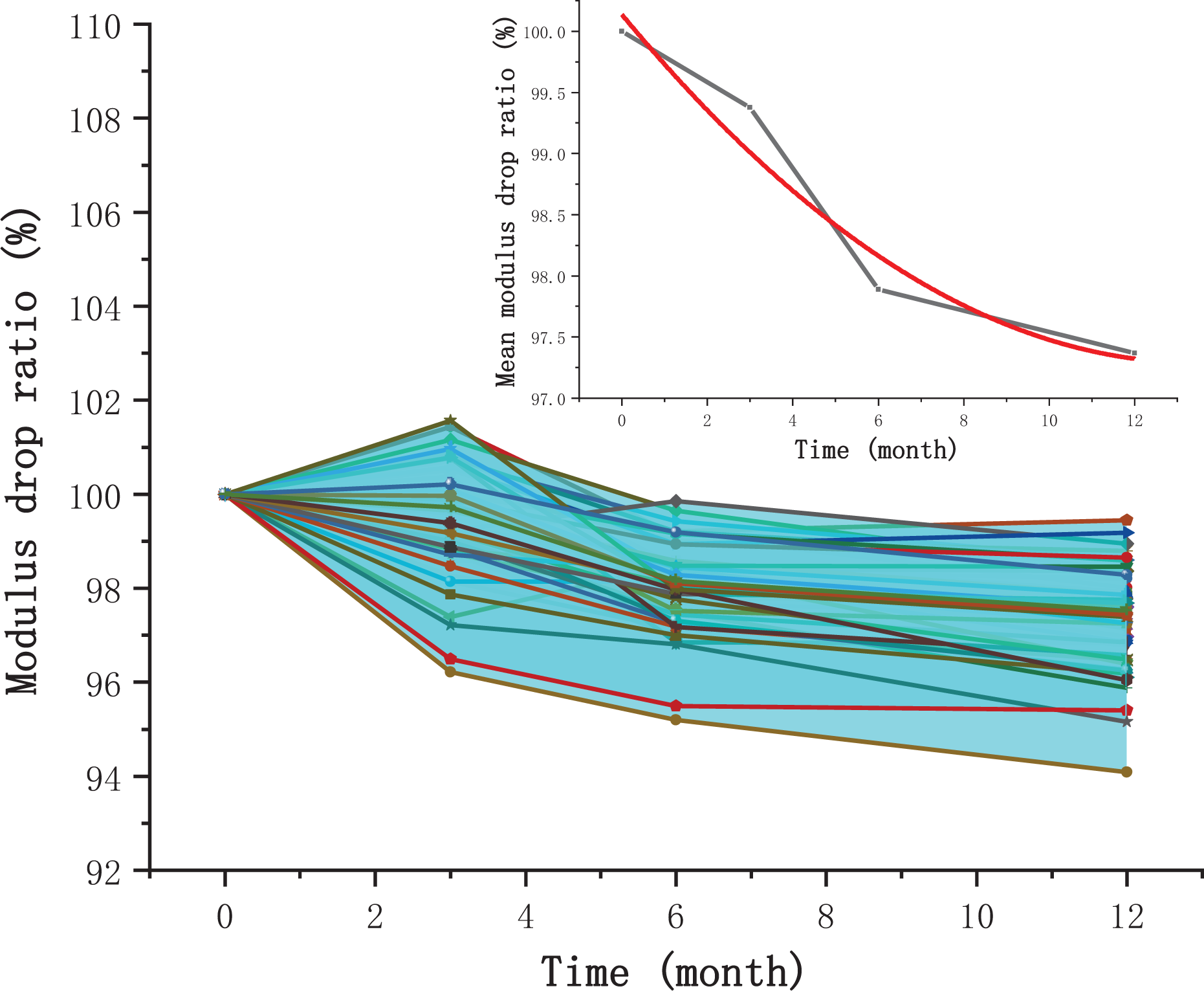
Elastic modulus-time in the hygrothermal environment (SNFT).

The average elastic modulus is fitted using a quadratic function. The results are given as follows

α = 1.57099 \times 10^{- 4} t^{2} - 0.00423 t + 1.00137

Figure 6 shows the ultimate strength–time relationship of destructive tests under the same conditions. The diagram includes the envelope diagram of the ultimate strength of all the specimens at different aging times and the average value of all the specimens. The width of the envelope diagram is smaller, and the data are more concentrated. The curves of the different specimens show a similar trend. The average ultimate strength of all the specimens indicates that the strength decreases significantly with an increase in the degraded time and then decreases slowly, which is similar to the trend of the elastic modulus. The polynomial fitting results are obtained as follows

α = 8.00109 \times 10^{- 4} t^{2} - 0.03482 t + 0.9908

Figure 6.

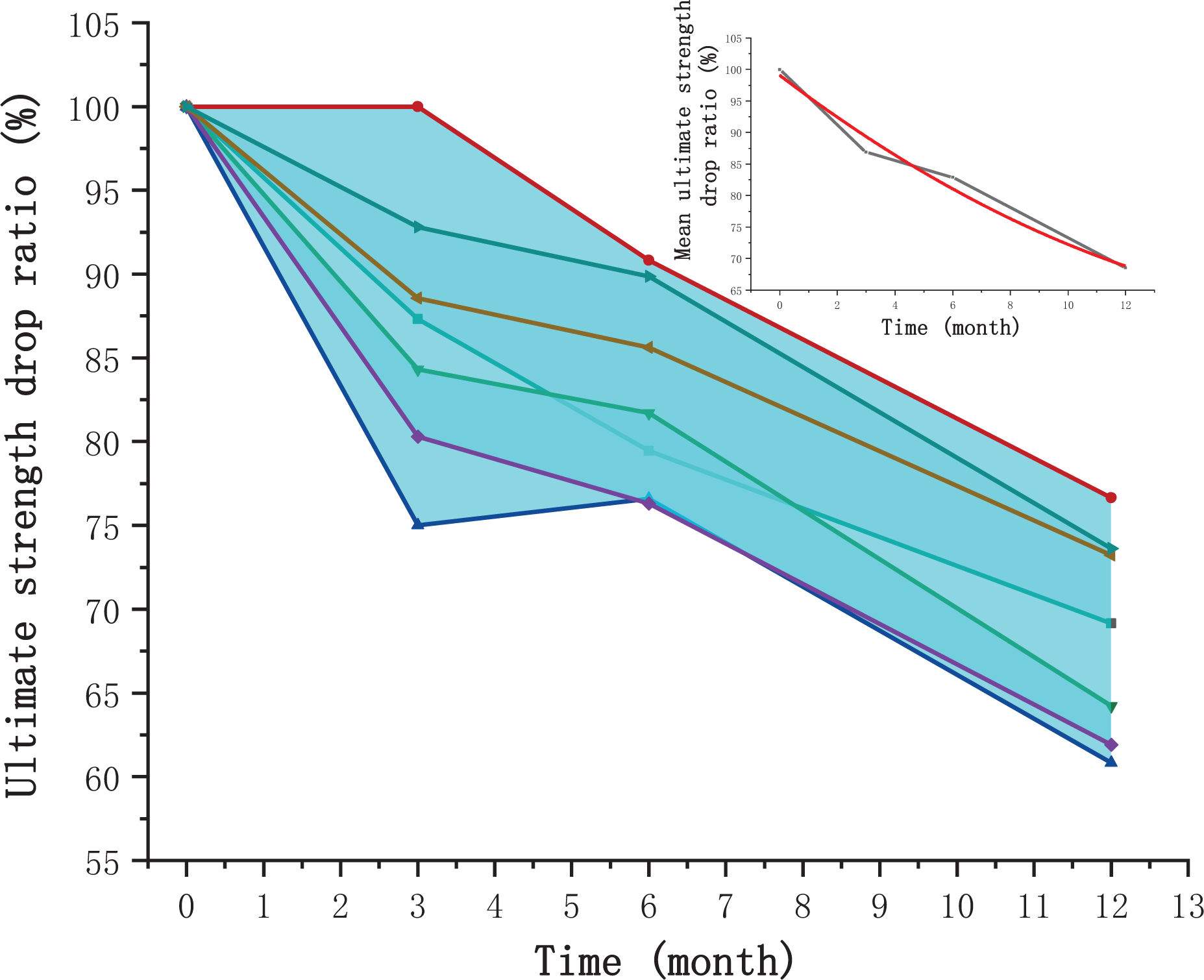
Ultimate strength-time in the hygrothermal environment (destructive test).

The average deviation of data from the SNFT and destructive tests according to equation (16) is calculated as follows

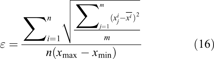
ε = \frac{\sum_{i = 1}^{n} \sqrt{\frac{\sum_{j = 1}^{m} {(x_{j}^{i} - \bar{x^{i}})}^{2}}{m}}}{n (x_{max} - x_{min})}

where i denotes the group i specimens, n is the total number of specimens, j represents the jth data point of the same specimen, and m is the total number of data points.

The calculation results are listed in Table 4.

Table 4.

Deviation table of humid and thermal environment data.

Test	SNFT	Destructive test
Test	SNFT	Ultimate strength	Elastic modulus
Deviation	0.0684	0.1455	0.2450

Based on the formula definition of data deviation, the proportion of average data deviation is within the data range. A smaller data deviation corresponds to a broader data range, a more significant effect of independent variables, smaller data variance, more stable results of different samples, and better test results. As shown in Table 4, SNFT yields higher data stability than the destructive test, and the calculated data from SNFT are comparatively more accurate.

GFRP-alkali

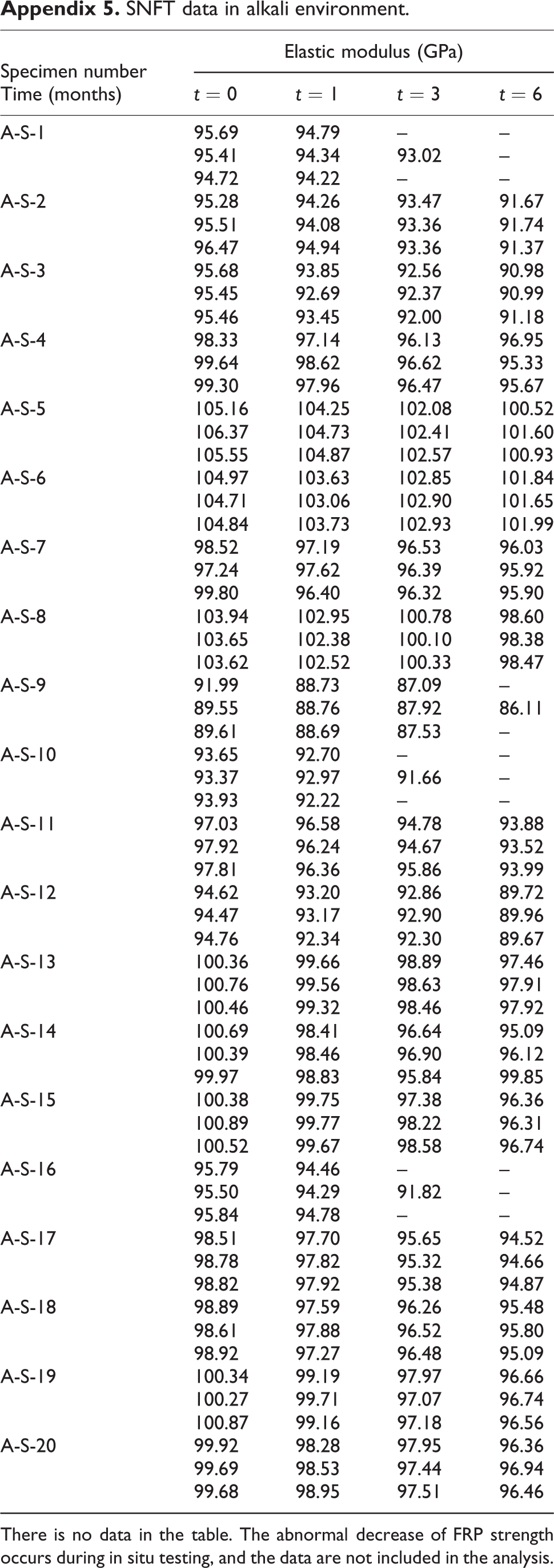
Appendix 4 shows the destructive test data of GFRP in the alkali environment, and Appendix 5 displays the SNFT test data of GFRP in alkali environment. Consistent with the test results of the hydrothermal environment, 28 specimens were used in the destructive test, of which 56 specimens were measured if the elongation data are neglected. The SNFT comprised 20 specimens from a total of 240 measured specimens. Similar to the case of the hydrothermal environment, SNFT is six times more efficient than destructive tests.

In Figure 7, the relationship between the decrease in elastic modulus of GFRP-SNFT and time in alkali solution is displayed, which includes each specimen’s elastic modulus at different degraded periods and the average value of all the specimens. Different specimens’ curves form the envelope diagram shown in the blue part. The envelope diagram width is small, the data are concentrated, and the curves of various specimens demonstrate a similar trend. The elastic modulus decreases gradually with the increase of degraded time based on the average elastic modulus. The decrease rate is faster during the early stage and the degraded rate reduces during the later stage.

Figure 7.

Elastic modulus-time in the alkali solution (SNFT).

A quadratic function can be used to fit the average elastic modulus, as follows

α = 9.062 \times 10^{- 4} t^{2} - 0.0116 t + 0.999

Figure 8 depicts the ultimate strength–time relationship of the destructive tests, including the ultimate strength envelope of all the specimens at different aging times and the average value of all the respective specimens. The width of the envelope is broader during the early stage than in the later stage, and the data of the early stage are more concentrated, whereas the discrete type in the later stage is comparatively higher. The curves of the various specimens demonstrate the same trend. The average ultimate strength of the specimens shows that with the increase of degraded time, the strength initially decreases rapidly, and later decreases slowly. The polynomial fitting results are expressed as follows

α = 0.01449 t^{2} - 0.18578 t + 1.03412

Figure 8.

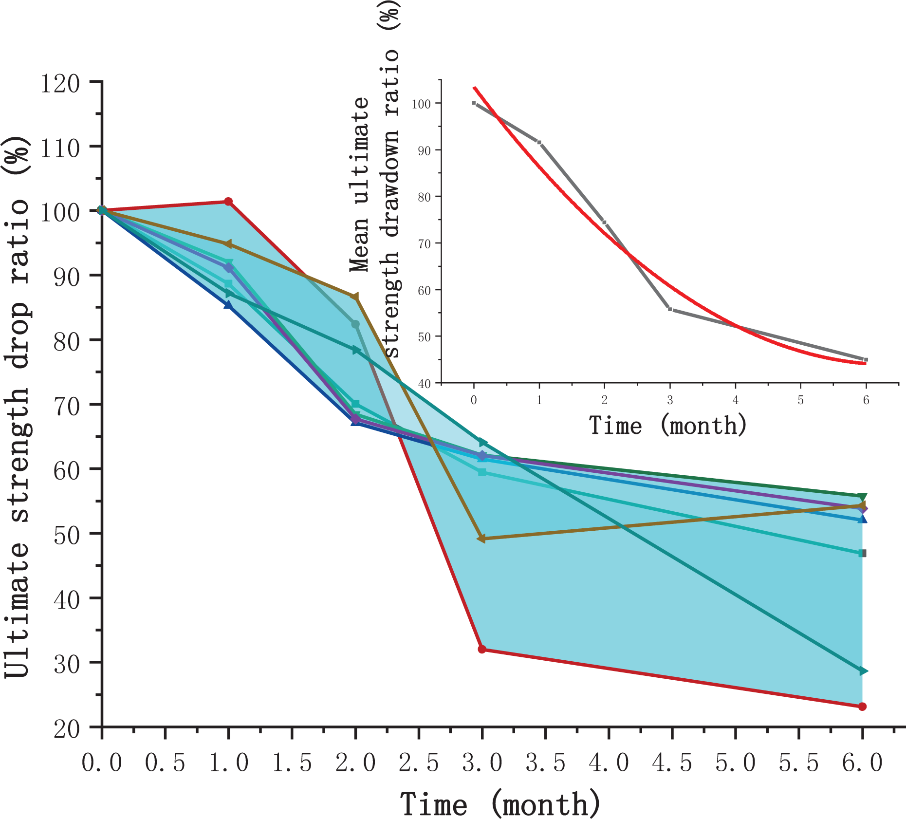
Ultimate strength-time in the alkali solution (destructive test).

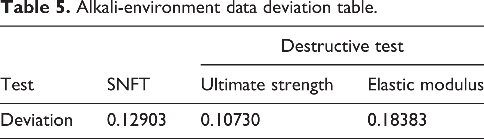
The average deviation between the SNFT and destructive test is calculated, and the results are obtained in the following.

From Table 5, the ultimate strength index data of the destructive test shows the smallest deviation. The data deviation of the SNFT is moderate, and the data regularity is significant. The elastic modulus index data of the destructive test exhibits the largest deviation.

Table 5.

Alkali-environment data deviation table.

Test	SNFT	Destructive test
Test	SNFT	Ultimate strength	Elastic modulus
Deviation	0.12903	0.10730	0.18383

Analysis and discussion

The curve is plotted by applying the ratio of elastic modulus drop as the horizontal axis and the ratio of ultimate strength drop as the vertical axis. The linear regression analysis is carried out, as presented in Figure 9.

Figure 9.

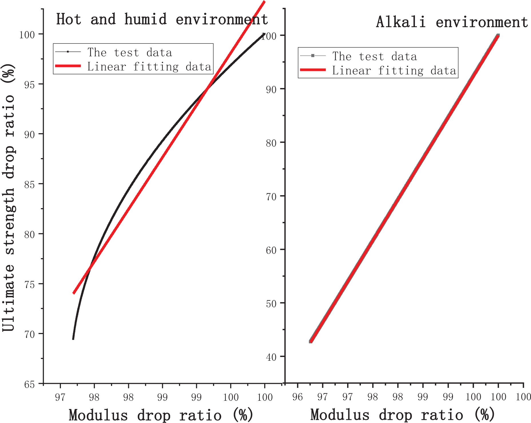
Elastic modulus–ultimate strength relationship.

Under the hydrothermal environmental condition, the fitting results of the linear regression analysis are obtained as follows

f_{r} = 10.42578 E_{r} - 9.39292

The relationship between the elastic modulus and ultimate strength is deduced from the model

f_{r} = γ E_{r} + 1 - γ

The slope and intercept can be solved as unknown variables: $γ = 0.09592$ . The fitting results for the alkali solution environment are given as follows

f_{r} = 15.32928 E_{r} - 14.32983

Similarly, the slope and intercept can be solved as unknown variables.

Result verification

SNFT data in the ultraviolet (UV) environment in reference are presented in Table 6 (Lan, 2018).

Table 6.

Test data in UV environment.

Aging time (h)	SNFT elastic modulus reduction ratio (%)	Ultimate strength reduction ratio of destructive test (%)
0	1	1
1080	1.02202	1.06821
2160	1.00172	1.02807
4320	0.98618	0.89300
6480	0.96977	0.78595
8640	0.9555	0.71993

UV: ultraviolet.

The relationship between the fitting elastic modulus and ultimate strength is given in Figure 10.

Figure 10.

Modulus–ultimate strength relationship (UV).

The fitting results are given as follows

f_{r} = 4.77067 E_{r} - 5.74859

The solution is $γ = 0.20961$ . Through theoretical and experimental fitting analyses, the relationship between the elastic modulus variation for SNFT and the variation in ultimate strength and degraded depth for the destructive test is obtained as follows

f_{r} = γ E_{r} + 1 - γ

E_{r} = 1 - (1 - β) \frac{d}{D}

f_{r} = 1 - (1 - α) \frac{d}{D}

The above equations are coupled with each other. Therefore, it is impossible to solve the degraded depth. It is necessary to know the proportion relationship between α and $β$ to obtain the degraded depth. α is the residual amount of ultimate strength in the degraded zone and ranges from 0 to 1; $β$ is the residual amount of elastic modulus in the degraded zone, also taken as 0–1. The relationship between the two can be obtained through experiments, and this is investigated in the next step. The correlation between the elastic modulus drop ratio and ultimate strength drop ratio can be obtained, which is related to the SNFT conversion coefficient. The value is related to the FRP type, environmental condition, FRP production process, and FRP formula. The working conditions measured in this study are described in Table 7.

Table 7.

Coefficient table under different working conditions.

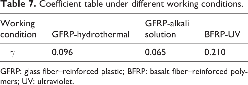
Working condition	GFRP-hydrothermal	GFRP-alkali solution	BFRP-UV
$γ$	0.096	0.065	0.210

GFRP: glass fiber–reinforced plastic; BFRP: basalt fiber–reinforced polymers; UV: ultraviolet.

Due to the lack of SNFT data, the destructive test data obtained by scholars are collected and counted. Using the elastic modulus and ultimate strength data obtained from the destructive test, the SNFT-failure conversion coefficients of different materials under different working conditions are calculated and listed in Table 8.

Table 8.

SNFT-failure conversion coefficient table.

	AFRP	BFRP	CFRP	GFRP
Water	–	–	0.63	0.92
Alkali	–	–	0.67	0.08
Acid	–	–	0.59	0.97
Hydrothermal	5.31	1.23	0.72	0.08

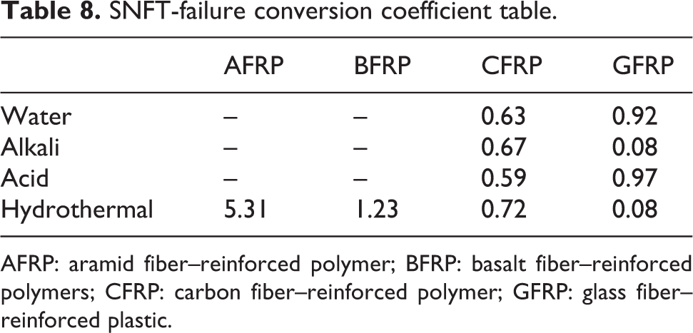
AFRP: aramid fiber–reinforced polymer; BFRP: basalt fiber–reinforced polymers; CFRP: carbon fiber–reinforced polymer; GFRP: glass fiber–reinforced plastic.

Conclusion

In this article, a mechanical model of FRP after degradation was presented, and the conversion relationship between the elastic modulus reduction ratio and ultimate strength reduction ratio was established. The SNFT method is proposed for assessing the durability of FRPs. The characteristics of the SNFT and traditional test methods are analyzed and compared. The following conclusions are drawn:

The SNFT method is feasible for measuring the elastic modulus, and the method can be used to characterize the degradation of FRPs under different environmental conditions.

The proposed conversion model conforms to the mechanical law and can express the change in material properties under different working conditions. The conversion coefficient can be generalized and has strong adaptability.

Compared with the destructive test, the elastic modulus data measured using the SNFT method is more centralized and regular.

SNFT can accurately express the degraded rule of FRP, transform with destructive testing, and obtain degraded depth data.

Footnotes

Acknowledgements

The authors sincerely appreciate the help and professional advice of Biao Li, Jie Lian, Jinjie Zhao, and Ao Guo.

Declaration of conflicting interests

The author(s) declared no potential conflicts of interest with respect to the research, authorship, and/or publication of this article.

Funding

The author(s) disclosed receipt of the following financial support for the research, authorship, and/or publication of this article: The authors would like to acknowledge the financial support provided by the National Natural Science Foundation of China (grant number 51678579).

ORCID iD

WenXiao Li

Appendix 5.

SNFT data in alkali environment.

Specimen number	Elastic modulus (GPa)
Time (months)	t = 0	t = 1	t = 3	t = 6
A-S-1	95.69	94.79	–	–
	95.41	94.34	93.02	–
	94.72	94.22	–	–
A-S-2	95.28	94.26	93.47	91.67
	95.51	94.08	93.36	91.74
	96.47	94.94	93.36	91.37
A-S-3	95.68	93.85	92.56	90.98
	95.45	92.69	92.37	90.99
	95.46	93.45	92.00	91.18
A-S-4	98.33	97.14	96.13	96.95
	99.64	98.62	96.62	95.33
	99.30	97.96	96.47	95.67
A-S-5	105.16	104.25	102.08	100.52
	106.37	104.73	102.41	101.60
	105.55	104.87	102.57	100.93
A-S-6	104.97	103.63	102.85	101.84
	104.71	103.06	102.90	101.65
	104.84	103.73	102.93	101.99
A-S-7	98.52	97.19	96.53	96.03
	97.24	97.62	96.39	95.92
	99.80	96.40	96.32	95.90
A-S-8	103.94	102.95	100.78	98.60
	103.65	102.38	100.10	98.38
	103.62	102.52	100.33	98.47
A-S-9	91.99	88.73	87.09	–
	89.55	88.76	87.92	86.11
	89.61	88.69	87.53	–
A-S-10	93.65	92.70	–	–
	93.37	92.97	91.66	–
	93.93	92.22	–	–
A-S-11	97.03	96.58	94.78	93.88
	97.92	96.24	94.67	93.52
	97.81	96.36	95.86	93.99
A-S-12	94.62	93.20	92.86	89.72
	94.47	93.17	92.90	89.96
	94.76	92.34	92.30	89.67
A-S-13	100.36	99.66	98.89	97.46
	100.76	99.56	98.63	97.91
	100.46	99.32	98.46	97.92
A-S-14	100.69	98.41	96.64	95.09
	100.39	98.46	96.90	96.12
	99.97	98.83	95.84	99.85
A-S-15	100.38	99.75	97.38	96.36
	100.89	99.77	98.22	96.31
	100.52	99.67	98.58	96.74
A-S-16	95.79	94.46	–	–
	95.50	94.29	91.82	–
	95.84	94.78	–	–
A-S-17	98.51	97.70	95.65	94.52
	98.78	97.82	95.32	94.66
	98.82	97.92	95.38	94.87
A-S-18	98.89	97.59	96.26	95.48
	98.61	97.88	96.52	95.80
	98.92	97.27	96.48	95.09
A-S-19	100.34	99.19	97.97	96.66
	100.27	99.71	97.07	96.74
	100.87	99.16	97.18	96.56
A-S-20	99.92	98.28	97.95	96.36
	99.69	98.53	97.44	96.94
	99.68	98.95	97.51	96.46

There is no data in the table. The abnormal decrease of FRP strength occurs during in situ testing, and the data are not included in the analysis.

References

ACI 440.3R:2004 (2004) Guide test methods for fiber-reinforced polymers (FRPs) for reinforcing or strengthening concrete structures.

Al-Safy

Al-Mahaidi

Simon

, et al. (2014) Thermo-mechanical characterization of VGCF-modified adhesive for bond between CFRP and concrete subjected to combined effect of temperature and humidity. Advances in Structural Engineering 17(12): 1718–1823.

Ceroni

Cosenza

Gaetano

, et al. (2006) Durability issues of FRP rebars in reinforced concrete members. Cement and Concrete Composites 28(10): 857–868.

Chen

Davalos

Ray

, et al. (2007) Accelerated aging tests for evaluations of durability performance of FRP reinforcing bars for concrete structures. Composite Structures 78(1): 101–111.

D’Antino

Pisani

(2018) Influence of sustained stress on the durability of glass FRP reinforcing bars. Construction and Building Materials 187: 574–486.

Dong

Zhao

, et al. (2018) Durability test on the flexural performance of seawater sea-sand concrete beams completely reinforced with FRP bars. Construction and Building Materials 192: 671–682.

Frigione

Lettieri

(2018) Durability issues and challenges for material advancements in FRP employed in the construction industry. Polymers 10(3): 247.

GB/T 3354:2014 (2014) Test method for tensile properties of oriented fiber reinforced polymer matrix composites.

Xian

Zhang

(2020) Effect of moderately elevated temperatures on bond behaviour of CFRP-to-steel bonded joints using different adhesives. Construction and Building Materials 241: 118057.

10.

Hedayat

Baniasadizade

(2015) Evaluation of the different test methods of the concrete durability for the Persian Gulf environment. Advances in Structural Engineering 18(10): 1575–1586.

11.

Karbhari

(2009) Durability of FRP composites for civil infrastructure myth, mystery or reality. Advances in Structural Engineering 6(3): 243–255.

12.

Kim

Park

You

, et al. (2008) Short-term durability test for GFRP rods under various environmental conditions. Composite Structures 83(1): 37–47.

13.

Lan

(2018) Study on Ultraviolet Durability of Basalt Fiber Sheets. Mianyang, China: Southwest University of Science and Technology.

14.

Gao

Huang

(2009) Durability of carbon fiber and glass fiber reinforced polymer composites. Journal of Harbin University of Technology 64(2): 150–154.

15.

Liang

, et al. (2019) The combined effects of wet–dry cycles and sustained load on the bond behavior of FRP–concrete interface. China Polymer Composites 40(3): 50–52.

16.

Ouyang

Wan

(2010) An analytical model of FRP-concrete bond deterioration in moist environment. Advances in Structural Engineering 12: 761–769.

17.

Pan

Xian

(2019) Influence of long-term outdoor exposure in a frigid zone on the CFRP-to-concrete bond behavior. Construction and Building Materials 215: 462–474.

18.

Pan

Shi

Xian

(2019) Experimental and numerical study of the CFRP-to-concrete bonded joints after water immersion. Composite Structures 218: 95–106.

19.

Prabhakar

Rajini

Ayrilmis

, et al. (2019) An overview of burst, buckling, durability and corrosion analysis of lightweight FRP composite pipes and their applicability. Composite Structures 230: 111419.

20.

(2013) Effects of UVA ultraviolet radiation on properties of indoor carbon fiber reinforced epoxy resin matrix composites. China Composites 30(2): 45–65.

21.

Yang

(2010) Durability of fiber reinforced polymer (FRP). China Building Materials Science and Technology 2010: 73–77.

22.

Yang

Jia

(2018) Control methods for non-destructive test of fiberglass sheets. China Industrial Buildings 48(3): 41–45.

23.

(2018) Experimental Study on Durability of Glass Fibre Sheets in Hot and Humid Environment. Mianyang, China: Southwest University of Science and Technology.