Experimental and numerical study on vortex-induced vibration of a truss girder with two decks

Abstract

Vortex-induced vibration (VIV) depends on aerodynamic shapes of bridge girders, which should be treated carefully in the design of long-span bridges. This paper studies the VIV performance of a suspension bridge with the truss girder which contains two separated decks. Although truss girders generally show better VIV performance than box girders, significant vibrations of this type of girders occurred in the wind tunnel tests based on a large-scale sectional model. Several lock-in regions with the same vibration frequency were observed, corresponding to different shedding vortices. Computational fluid dynamics (CFD) simulations were carried out, and monitoring points were set behind different components to study the characteristics of the shed vortices. As the truss girder consists of many members, the results show that various vortices with different dominant frequencies are formed in the wake flow. The vertical VIV of the bridge is probably driven by the vortices behind or above the upper deck, which is related to the guardrails. The torsional VIV of the bridge is probably driven by the vortices behind or below the lower deck, which is related to the service road at lower wind speeds while may be related the vertical stabilizers at higher wind speeds.

Keywords

CFD simulations suspension bridge truss girder with two decks vortex-induced vibration vortex shedding characteristics wind tunnel tests

Introduction

Long-span bridges are more sensitive to wind loads due to their flexible structural characteristics, and the wind-induced vibration has become an important issue. Vortex-induced vibration (VIV) is one of the typical wind-induced vibrations of bridges. It is a fluid-solid coupling phenomenon caused by alternate vortices shed from the girder or other components like tower columns and cables. The frequency of the alternate vortices, which increases with the increase in wind speed, may be locked when approaching the structural natural frequencies, that is, the lock-in phenomenon. Unlike the flutter instability which may drive a bridge to divergent vibration, the VIV leads to limited amplitudes in general but is closely related to the safety of structures as well as running vehicles.

There have been several incidents corresponding to the vortex-induced vibration of bridges, such as the Kessock Bridge (Owen et al., 1996), the Wye Bridge (Smith, 1980), the Rio-Niteroi Bridge with a continuous steel twin-box girder (Battista and Pfeil, 2020), the Great Belt Bridge with a streamlined box girder (Larsen et al., 2000), the Trans-Tokyo Bay Crossing Bridge with a straight ten-span continuous steel box-girder (Fujino and Yoshida, 2002), the Second Severn Crossing Bridge with a steel-concrete composite girder (Macdonald et al., 2002), the Volgograd Bridge with a continuous steel box girder (Corriols and Morgenthal, 2012), and the Xihoumen Bridge with a separated twin-box girder (Li et al., 2011). With the further increase in bridge span, it is more necessary to understand the VIV performance of bridges and how to ensure their safety.

The studies on the VIV performance of bridges mainly focus on box girders (e.g. Chen et al., 2017; Larsen, 1995; Li et al., 2018b; Ma et al., 2018; Mashnad and Jones, 2014; Nagao et al., 1997; Wang et al., 2019). With the extending of bluff bodies, a noteworthy phenomenon is the presence of more than one vortex migrating across the width direction, leading to the occurrence of more than one VIV peak (Deniz and Staubli, 1997; Nakamura and Nakashima, 1986). Naudascher and Wang (1993) pointed out that rectangular prisms are susceptible to three types of vortex-induced vibrations caused by leading-edge vortex shedding, impinging leading-edge vortices, and trailing-edge vortex shedding. Hourigan et al. (2001) indicated that the natural flow around rectangular plates is of greater complexity due to the interaction between the leading- and trailing-edge shedding.

Truss girders of bridges consist of many discrete components. For bridge decks with larger widths, more than one vortex may migrate across the width direction, as discussed above for extended bluff bodies. Meanwhile, different components of truss girders show different bluff-body aerodynamic characteristics, causing various vortices with different sizes and shedding frequencies which complicate the VIV performance of truss girders. Furthermore, the distances among some components of truss girders change continuously along the bridge axis, leading to complex aerodynamic interference. Oh et al. (2018) proposed a method for predicting wind velocity at which VIV occurs on a road-rail bridge with truss girder. Tang et al. (2019) found that the wake of the upstream components is more related to the VIV of the truss girder as it may inhibit the vortices shed from the downstream components. Compared with box girders, the VIV performance of truss girders is harder to evaluate and has not yet been fully explored, calling for further investigations.

A long-span suspension bridge with a truss girder with two decks is taken as the example. The girder has a relatively uniform aerodynamic shape as the cross-section has small changes along the bridge axis. The aim of this paper is to study the VIV performance of this type of girders, and understand the probable reason driving the girder to the VIV, and the main content is organized as follows. In section 2, the structural dynamic characteristics of the bridge are introduced. In section 3, the lock-in phenomenon and the VIV amplitude of the girder are studied by wind tunnel tests with a sectional model. In section 4, the shedding characteristics of various vortices in the wake are investigated by computational fluid dynamics (CFD) simulations. Finally in section 5, some conclusions are drawn.

Structural dynamic characteristics

The target bridge is a suspension bridge supported by three towers. The total length is about 2178 m and two main spans have the length of 800 m, as shown in Figure 1. The bridge is situated at the mouth of the Oujiang River flowing into the East China Sea. Compared with mountainous areas where wind parameters varies along the bridge axis (Tang et al., 2020), the uniform approaching flow may be more unfavorable to the VIV performance of the bridge. The finite element software ANSYS was adopted to compute the structural dynamic characteristics of the suspension bridge. A three-dimensional (3D) finite element model was established, as shown in Figure 2.

Figure 1.

Schematic layout of a (230 + 800 + 800 + 348) m suspension bridge (unit: m).

Figure 2.

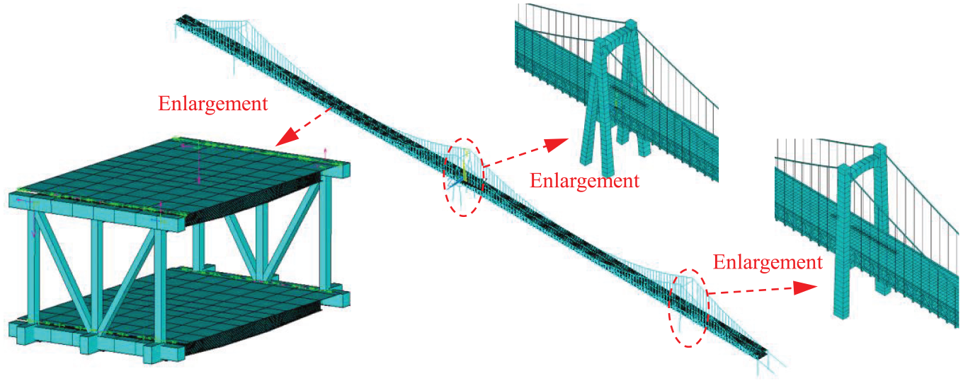
Three-dimensional finite element model and local enlargements.

The stiffening girder was simulated by the combination of beam and plate-shell elements. Specially, the chord members and the diagonal bracing members of the truss were simulated by Beam4 elements. The cross girders were simulated by Beam188 elements. The bridge deck was simulated by Shell63 elements. Other affiliated members were simulated by Mass21 elements, including the guardrails for vehicles, the service roads for maintenance workers, and the maintenance tracks for the inspection vehicle. The towers and the piers were simulated by Beam4 elements and fixed at their bottoms. The cables and the suspenders were simulated by LINK8 elements. A total of 390 cables were established, and the initial stress and the sag effect were considered. The dynamic characteristics of the bridge are solved by the modal analysis of ANSYS, which takes into account the large deformation and stress stiffening effect. The natural frequencies of some typical modes are listed in Table 1.

Table 1.

Main modal frequencies and the corresponding modal shapes of the bridge.

Order number	Vibration mode	Frequency (Hz)
3	AS-V-1	0.168
5	S-V-1	0.210
6	AS-V-2	0.227
7	S-V-2	0.261
30	AS-T-1	0.608
33	S-T-1	0.632

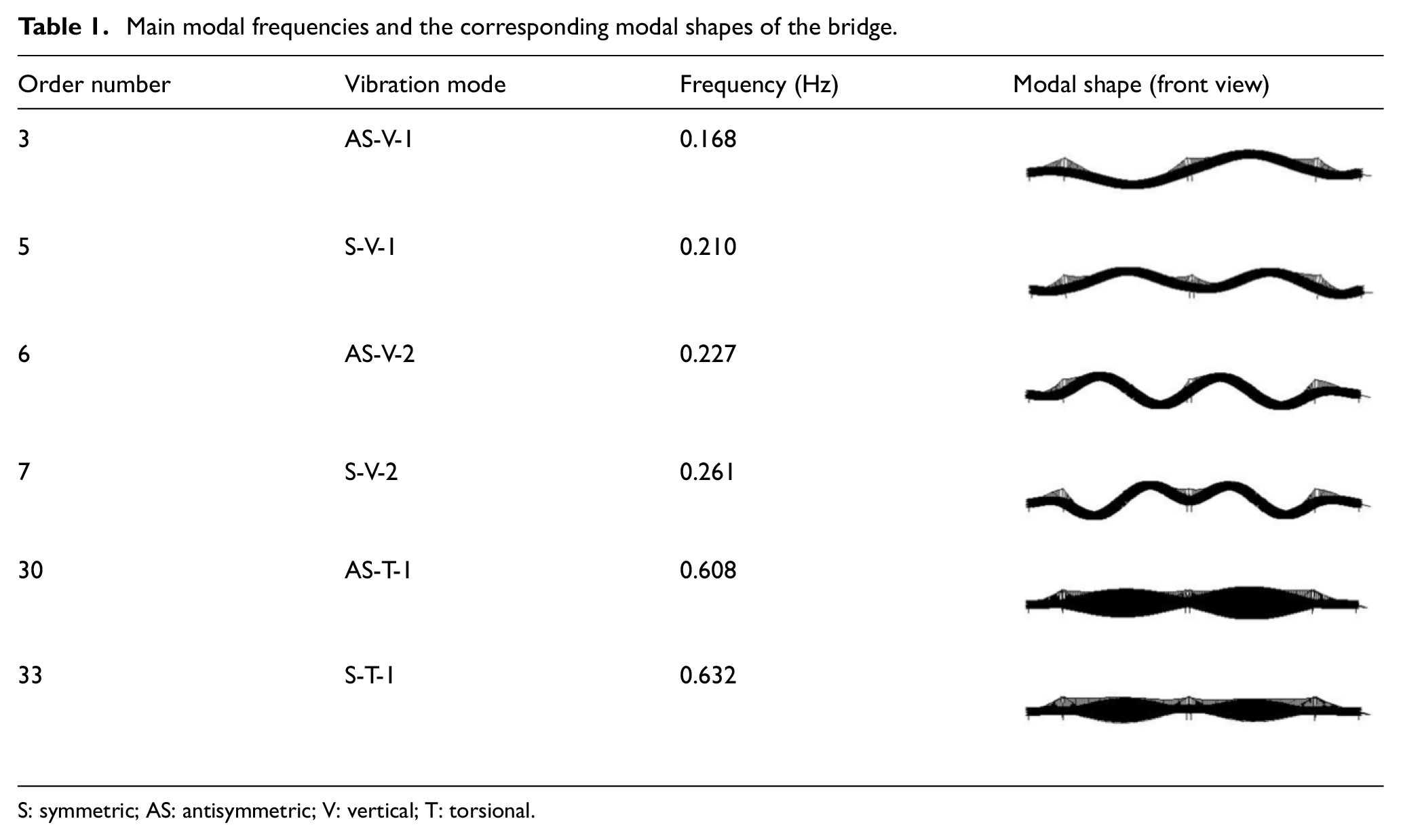
S: symmetric; AS: antisymmetric; V: vertical; T: torsional.

Vortex-induced vibration phenomenon by wind tunnel tests

A wind tunnel test program was implemented to study the vortex-induced vibration performance of the suspension bridge. The tests were conducted in XNJD-3 wind tunnel with a dimension of 22.5 m (width) × 4.5 m (height) × 36 m (length). The turbulence intensity in the empty tunnel was less than 1.0%. Uniform approaching conditions were simulated in the tests. In the middle of the tunnel, two internal guide wall with streamlined shapes, between which was suspended the sectional model, were set.

Sectional model in the wind tunnel tests

The aerodynamic shape of the experimental model referred to that of the girder of the target bridge strictly. The truss girder supported two orthotropic bridge decks on the upper and lower sides. Two main chords were embedded in each bridge deck on the left and the right sides, which increases the integrity of the main girder. The standard cross-section of the steel truss stiffening girder is shown in Figure 3. In order to improve the flutter stability of the bridge, several vertical stabilizers were designed below the lower deck (Li et al., 2018a). The stabilizers are longitudinal plates and 1.75 m deep running the length of the girder to disrupt the circulation of vortices. Except for the diagonal bracing members, the model had a relatively uniform aerodynamic shape as the cross-section has small changes along the bridge axis.

Figure 3.

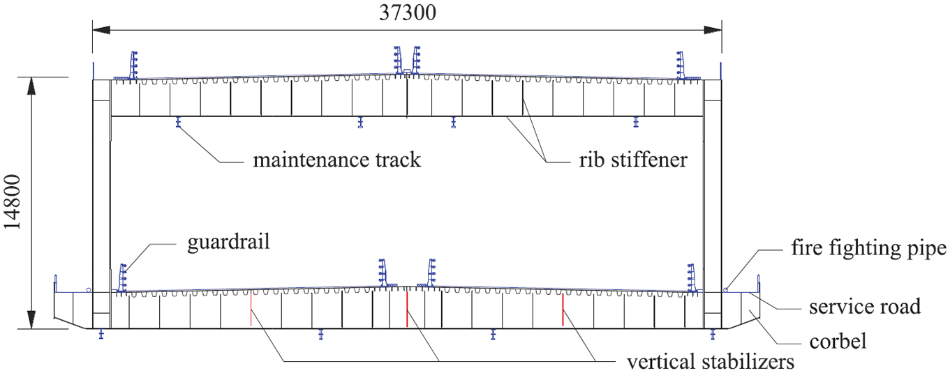
Standard cross-section of the steel truss stiffening girder (unit: mm, red lines: vertical stabilizers, blue lines: secondary elements).

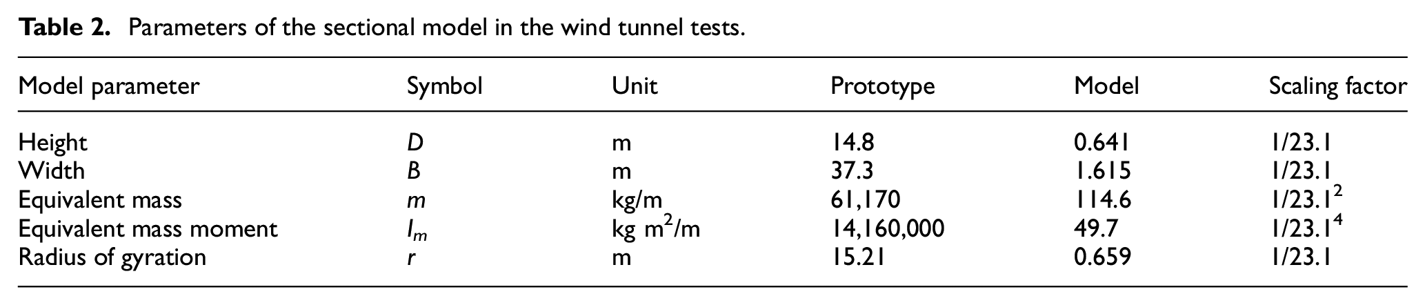
The geometric scale ratio of the experimental model to the real bridge was 1/23.1. The width of the model B was 1.615 m and the height D was 0.641 m. The length of the model was 3.46 m, as shown in Figure 4. The scaling factors for the section model is shown in Table 2. The use of the large scale ratio not only increased the accuracy of the model itself, but also reduced the effect of the change in Reynolds number, which is favorable to evaluate the VIV performance of the bridge.

Table 2.

Parameters of the sectional model in the wind tunnel tests.

Model parameter	Symbol	Unit	Prototype	Model	Scaling factor
Height	D	m	14.8	0.641	1/23.1
Width	B	m	37.3	1.615	1/23.1
Equivalent mass	m	kg/m	61,170	114.6	1/23.1²
Equivalent mass moment	I_m	kg m²/m	14,160,000	49.7	1/23.1⁴
Radius of gyration	r	m	15.21	0.659	1/23.1

Figure 4.

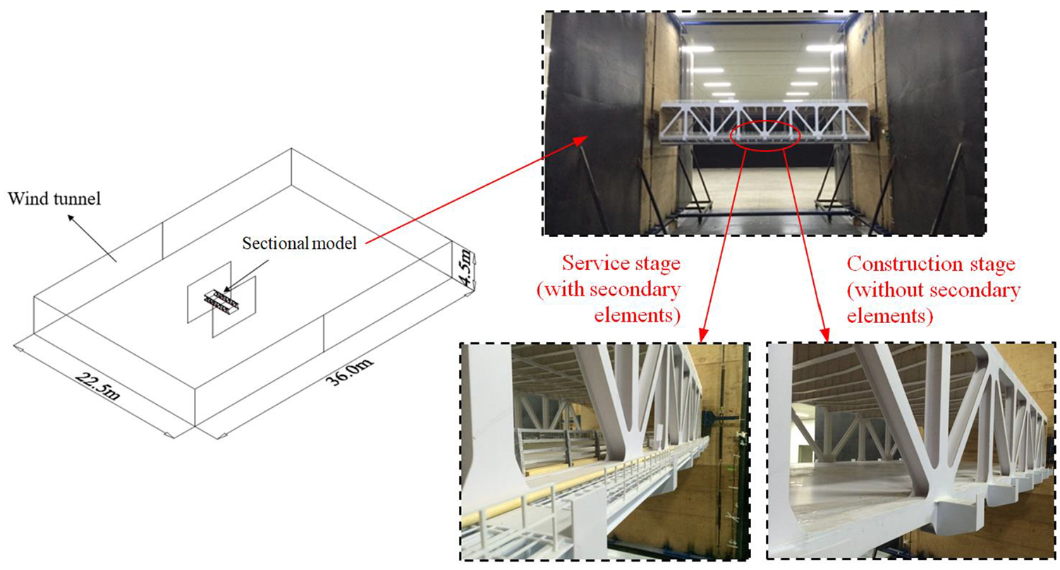
Large-scale sectional model in the wind tunnel and local enlargements.

Experimental set-up

The sectional model was fixed to two steel brackets which are hanged by eight springs installed at the end plate. Generally, VIV of bridges occurs at lower wind speeds. In order to reduce the wind speed ratio of the real value to the experimental value, relatively rigid springs were used to increase the vibration frequency of the model, and the wind speed ratio of the real value to the experimental value decreased. Figure 5 shows the suspension system. Specifically, the equivalent mass and the equivalent mass moment of inertia of the model were 103.5 kg/m and 41.3 kg m² per meter, and the corresponding radius of gyration was 0.632. These values were slightly smaller than the requirements, as shown in Table 2. The vertical and torsional frequencies of the model were 2.58and 4.18 Hz, respectively, so the wind speed ratios of the real value to the experimental value were 1.51 and 3.36 in the two directions. The damping ratios of the model in vertical and torsional directions were 0.15% and 0.31%, respectively. 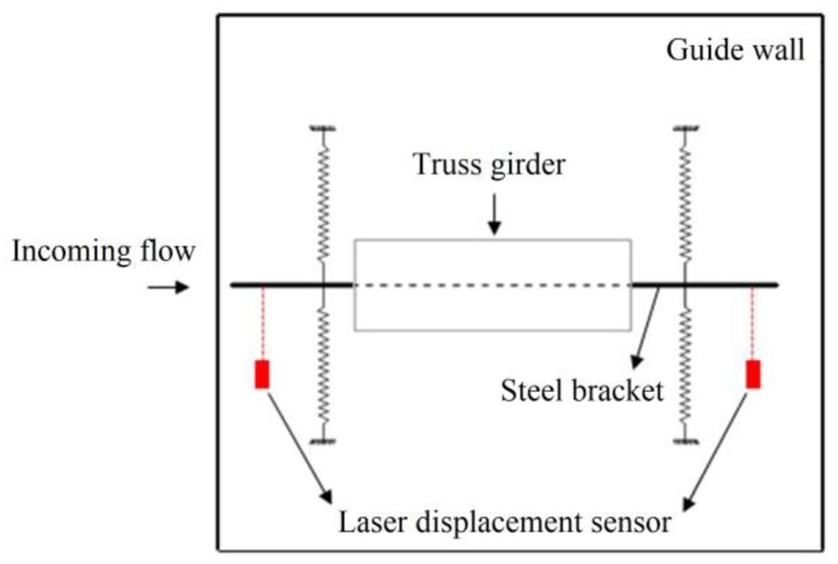The Scruton number defined as $Sc = 4 π m ξ / (ρ D^{2})$ was 5.9, where $ξ$ is set to the mean damping ratio in the two directions, $ρ$ is the air density, and other parameters are shown in Table 2. The target value was 14.3, and the difference was caused by the small damping ratio. It should be noted that the reference cross-wind width D is obviously larger than the actual cross-wind widths of the truss members.

Figure 5.

Suspension system of the experimental model in the wind tunnel tests.

Results and discussion

Tests were carried out under the attack angles of 0°, +3°, and −3°, respectively. The wind velocity of the incoming flow in the tunnel was increased gradually, and the wind-induced vibration of the model was recorded by a pair of laser displacement sensors. For the bridge in the service stage, the root mean square (RMS) displacements in the vertical and the torsional directions versus the wind speed U are shown in Figure 6(a) and (b) where the values correspond to the real bridge.

Figure 6.

RMS displacements of the bridge versus wind speeds corresponding to the real situation: (a) in vertical direction and (b) in torsional direction.

A lock-in range with significant larger amplitudes and another lock-in range with smaller amplitudes can be seen for both the vertical VIV and the torsional VIV, and they are called the major and the minor lock-in ranges in the following. At the three tested angles of attack, the major lock-in ranges for the vertical VIV or the torsional VIV are almost the same, while the minor lock-in ranges are different. The vertical and the torsional RMS displacements of the bridge within the major lock-in ranges are significant. For the bridge in the construction stage, the RMS displacements in the two directions are shown in Figure 6(c) and (d). The possible lock-in wind speeds of the bridge in the construction stage are computed according to the Strouhal numbers corresponding to the major lock-in ranges in the service stage. Without the secondary elements, no lock-in range is observed in the construction stage, which indicates that the VIV phenomenon in the service stage probably depends on the secondary elements. It is worth noting that the torsional displacement increases again when the wind speed approaches to 30 m/s. The wind speed, which is generally larger than the allowable wind speed for vehicle driving, was not further increased due to the smaller wind speed ratio.

Taking 0° attack angle as an example, Figure 7 shows the time series of the displacements at the two measurement points and the corresponding amplitude spectra. As the vertical VIV occurs at the wind speeds of 3.64 and 6.18 m/s, the two time series tested by the two sensors have the same phase. The lock-in wind speeds are different but the dominant frequencies of the vibration are the same, that is, 2.625 Hz, which is close to the vertical frequency of the experimental model. Similarly, with the wind speeds of 11.26 and 16.26 m/s, the torsional VIV occurs with the same frequency, that is, 4.250 Hz, which is close to the torsional frequency of the model. Furthermore, the torsional vibration occurs again when the wind speed increases to 29.13 m/s. The vibration is also caused by shedding vortices because it has the same dominant frequency of 4.250 Hz. The above phenomenon indicates that a vertical mode or a torsional mode of the bridge may be driven to VIV by different vortices with different shedding frequencies.

Figure 7.

Time series and amplitude spectrums of the displacements at different wind speeds corresponding to the real situation: (a) U = 3.64 m/s, (b) U = 6.18 m/s, (c) U = 11.26 m/s, (d) U = 16.26 m/s, and (e) U = 29.13 m/s.

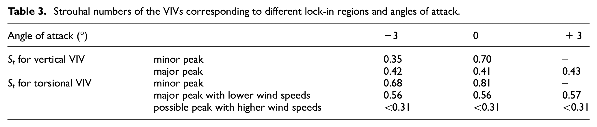
Considering different angles of attack, the lock-in wind speeds corresponding to different VIV peaks are listed in Table 3. For each case, the dominant frequency f is used for computing the Strouhal number S_t which is defined as S_t = fD/U. The results are shown in Table 3. The values of S_t corresponding to the major peaks are almost the same, while those corresponding to the minor peaks are different, which indicates that the main vortices driving the bridge to the significant VIV are little affected by the change in angle of attack. In addition, S_t is equal to 0.31 when the wind speed approaches to 29.13 m/s. As the RMS displacement of the bridge is still increasing, the lock-in wind speed is larger than 29.13 m/s and the correct value of S_t should be less than 0.31.

Table 3.

Strouhal numbers of the VIVs corresponding to different lock-in regions and angles of attack.

Angle of attack (°)		−3	0	+3
S_t for vertical VIV	minor peak	0.35	0.70	–
S_t for vertical VIV	major peak	0.42	0.41	0.43
S_t for torsional VIV	minor peak	0.68	0.81	–
	major peak with lower wind speeds	0.56	0.56	0.57
	possible peak with higher wind speeds	<0.31	<0.31	<0.31

Vortex shedding characteristics by static numerical simulations

In order to determine the reason driving the bridge to VIV and explain the phenomenon that several lock-in regions correspond to the same vibration frequency, the wake characteristics of the truss girder are further investigated. As the truss girder consists of many components, it is very complicated to establish a three-dimensional (3D) model accurately, so two-dimensional (2D) CFD simulations were carried out. For the target truss girder, the variation of the cross-section along the span direction is mainly caused by the diagonal bracing members, as shown in Figure 8. In order to fully describe the wake characteristics, three cross sections were selected according to the arrangement of the diagonal bracing members, that is, 1-1, 2-2, and 3-3 for which the distances of the diagonal bracing members to the upper chord member are 0.25h, 0.5h, and 0.75h, respectively, where h is the distance between the centers of the upper chord and the lower chord members.

Figure 8.

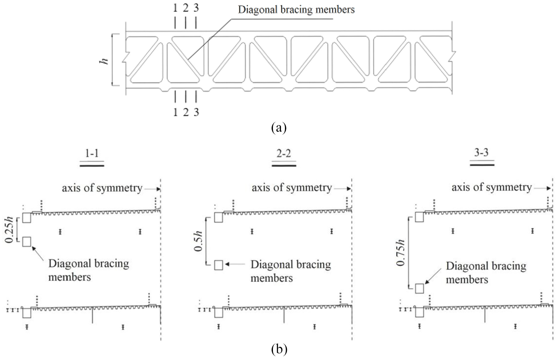
Three cases computed by CFD simulations: (a) front view of the truss girder and (b) side view of the truss girder (half the cross-section).

The two-dimensional (2D) models were established because of the efficiency and simplicity. 2D CFD simulations were widely used for evaluating the aerodynamic performance of bridges. Some components of the truss girder were not considered as they are discontinuous along the bridge span, such as the corbel, the rib stiffener, as shown in Figure 3. The CFD models had the same scale ratio as the experimental model, that is, 1/23.1. To simulate the aerodynamic characteristics of the truss girder accurately, the models were established according to the following principles, that is, the same aerodynamic shape for all members, the equivalent total area acted by wind for vertical members, and the similar aerodynamic interference for horizontal members. Although some simplifications are made, it is an efficient method to study the aerodynamic mechanism of wind-induced vibrations of truss girders (Tang et al., 2017, 2019).

Static CFD models

The computational domain and the boundary conditions used in this study are shown in Figure 9. The length and the height of the computational domain are 31D in the mean flow direction and 19D in the cross-flow direction, respectively. The blocking ratio of the model is 5.25% which is larger than its actual value due to the selection of D. The windward and the leeward sides were set as the velocity-inlet and the pressure-outlet boundaries, respectively, and the girder was set as the smooth wall. A boundary layer with three rows clinging to the girder was set to improve the mesh quality. The mesh size progressively increased from the internal boundary to the external boundaries, and the total cell number was 431,352.

Figure 9.

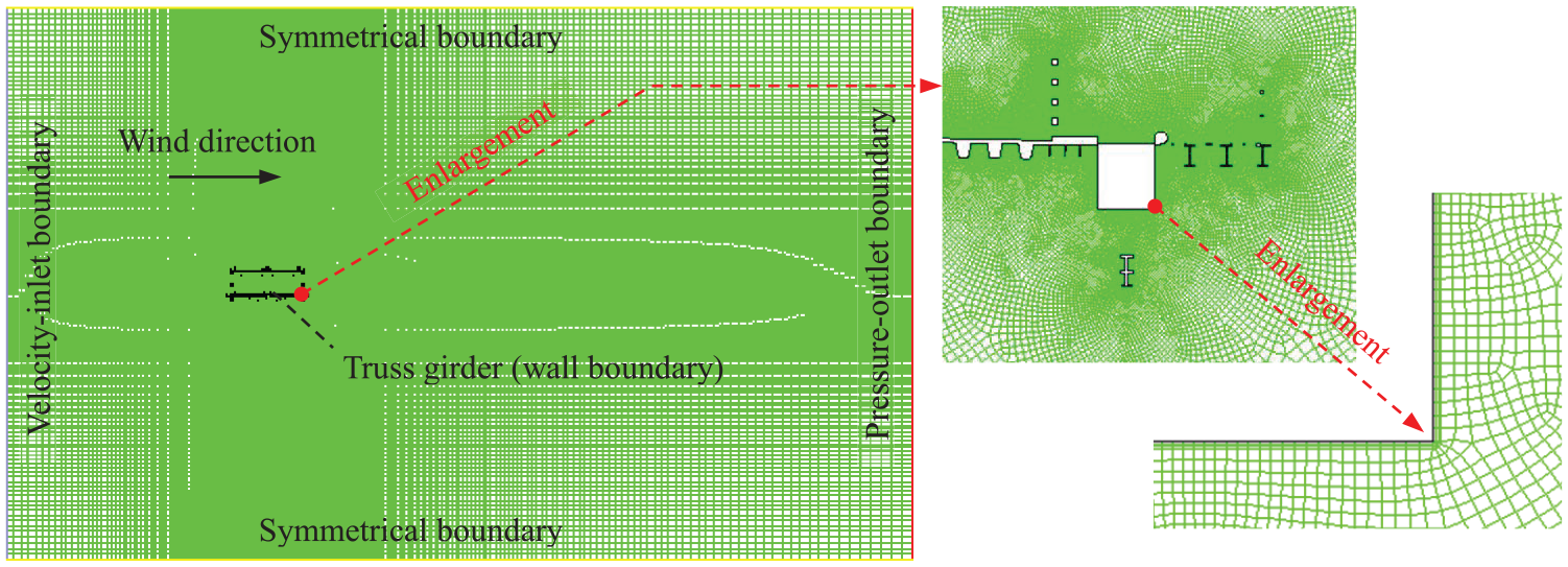
Computational domain and mesh employed in the CFD simulations.

Simulations were achieved by using the CFD software FLUENT. The k–ω shear stress transport (SST) model was adopted with unsteady Reynolds-averaged Navier–Stokes (URANS) simulations. The model could provide more accurate results, if compared to standard k–ω and k–ε models, in external aerodynamic cases which involve boundary layer separation (De Miranda et al., 2015). The SIMPLE pressure–velocity coupling algorithm was adopted to solve the discretized problem. The second-order upwind scheme was selected for momentum, turbulent kinetic energy, and specific dissipation rate.

The truss girder consists of many members with bluff aerodynamic shapes, producing large and small vortices with different frequencies. As discussed in the previous section, some vortices have strong influence on the girder, driving the bridge to the VIV with significant displacements. Other vortices have less influence on the girder which may drive the bridge to the VIV with small displacements. The SST k–ω model is one of the RANS models that the time-average process is used for the Navier–Stokes equation. Smaller unsteady flow characteristics will be offset if the time step is too large (Zhu, 2015). In order to capture these vortices accurately, it is very important to determine a suitable time step and a sufficient cell number. First, the time steps of 1 × 10⁻³, 5 × 10⁻⁴, 1 × 10⁻⁴, 5 × 10⁻⁵, and 1 × 10⁻⁵ were considered, and the wind speed of the incoming flow was set to 14 m/s with null attack angle. The drag, the lift, and the moment coefficients of the girder were computed, which are defined as C_D = F_D/(0.5ρU²D), C_L = F_L/(0.5ρU²B), and C_M = F_M/(0.5ρU²B²) where F_D, F_L, and F_M are the drag, the lift, and the pitching moment, respectively; ρ is the air density; U is the wind velocity; D and B are the height and the width with the reduced scale. The positive directions of the aerodynamic forces are shown in Figure 10.

Figure 10.

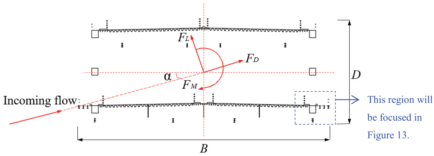
Definitions of the aerodynamic coefficients.

The data within ten vortex shedding cycles when the computation has converged are selected to compute the mean aerodynamic coefficients and their standard deviation values. The results are shown in Table 4. According to the results, the mean values and the standard deviation values of the cases with the time steps of 1 × 10⁻³ and 5 × 10⁻⁴ are smaller significantly than those of the other three cases. When the time step is 1 × 10⁻⁴, further decrease in time step has little effect on the results. Considering the accuracy and the efficiency, the time step of 1 × 10⁻⁴ will be adopted in the subsequent computation.

Table 4.

Comparisons of the aerodynamic coefficients with different time steps.

Time step (s)		1 × 10⁻³	5 × 10⁻⁴	1 × 10⁻⁴	5 × 10⁻⁵	1 × 10⁻⁵
Mean values	${\bar{C}}_{L}$	0.3297	0.3161	0.3840	0.3842	0.3844
	${\bar{C}}_{M}$	0.0040	0.0037	0.0301	0.0302	0.0303
	${\bar{C}}_{D}$	0.6999	0.7019	0.7975	0.7980	0.7985
Standard deviation values	$C_{L}^{'}$	0.0394	0.0254	0.0671	0.0670	0.0677
	$C_{M}^{'}$	0.0122	0.0198	0.0235	0.0230	0.0241
	$C_{D}^{'}$	0.0140	0.0222	0.0462	0.0466	0.0459

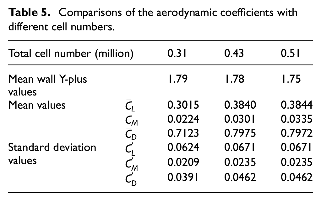
Subsequently, the effect of the total cell number on the aerodynamic coefficients of the cross-section is studied. The total cell number of 0.43 million was decreased to 0.31 million and increased to 0.51 million, respectively. The corresponding models were established. The mean values and the standard deviation values of the aerodynamic coefficients are shown in Table 5. Meanwhile, the mean wall Y-plus values around the truss girder are also shown to evaluate the spatial discretization. For the three cases, the Y-plus values are close to one another, while the aerodynamic coefficients show different. The cases with the cell numbers of 0.43 million and 0.51 million lead to similar results which are different from the results of the case with cell number of 0.31 million. Considering the accuracy and efficiency, the total cell number of 0.43 million will be adopted in the subsequent computations.

Table 5.

Comparisons of the aerodynamic coefficients with different cell numbers.

Total cell number (million)		0.31	0.43	0.51
Mean wall Y-plus values		1.79	1.78	1.75
Mean values	${\bar{C}}_{L}$	0.3015	0.3840	0.3844
	${\bar{C}}_{M}$	0.0224	0.0301	0.0335
	${\bar{C}}_{D}$	0.7123	0.7975	0.7972
Standard deviation values	$C_{L}^{'}$	0.0624	0.0671	0.0671
	$C_{M}^{'}$	0.0209	0.0235	0.0235
	$C_{D}^{'}$	0.0391	0.0462	0.0462

Vortex shedding characteristics

Taking 2-2 cross-section as the example, the wind velocity for the numerical computation was set to 5 m/s which is close to the lock-in wind speed of the major torsional VIV in the wind tunnel tests. To capture the vortex shedding characteristics more accurately, the computing time was extended and much more vortex shedding cycles could be considered. The mean wall Y-plus value around the truss girder further decreases to 0.76 when the computation has converged. For the whole girder, the time series of the lift and the moment coefficients are shown in Figure 11. Through the spectra analysis, several peak components can be observed. Their frequencies and the corresponding S_t are listed in Table 6. The shapes and the positions of the truss members are different, so various vortices with different sizes and shedding frequencies are easy to induce. The dominant frequency with the highest amplitude is 22.47 Hz corresponding to the peak number 9 for the lift coefficient and 8.94 Hz corresponding to the peak number 5 for the moment coefficient. With the dominant components, the predicted lock-in wind speeds in the wind tunnel tests should be 0.57 m/s for the vertical VIV and 2.33 m/s for the torsional VIV. Actually, no significant vibration was observed at the two predicted wind speeds, and the probable reason is that the wind speeds are relatively low and the input energy is small. With the increase in wind speed, however, the peak components with lower frequencies and amplitudes may drive the bridge to the VIVs.

Figure 11.

Time series and amplitude spectrums of the aerodynamic coefficients: (a) $C_{L}$ and (b) $C_{M}$ .

Table 6.

Characteristics of the peak components of the aerodynamic coefficients.

Peak number		1	2	3	4	5	6	7	8	9
Frequency (Hz)	${\bar{C}}_{L}$	1.86	3.60	5.46	8.82	–	9.93	12.79	17.76	22.47
Frequency (Hz)	${\bar{C}}_{M}$	1.86	3.60	5.46	–	8.94	–	12.79	–	22.47
Corresponding S_t		0.24	0.46	0.70	1.13	1.15	1.27	1.64	2.28	2.88

In order to find out the vortices driving the bridge to the VIVs, a total of 33 monitoring points were set up at different positions to record the wind velocities, as shown in Figure 12. The monitoring points P1 to P8 were set above the upper deck; P9 behind the upper deck; P11 and P14 below the upper deck; P10, P12, P13, and P15 behind the upper maintenance tracks; P16 behind the upper chord; P17 and P21 behind the diagonal bracing members; P18, P19, P20, and P22 above the lower deck; P23 behind the lower deck; P25 and P31 below the lower deck; P26, P28, and P30 behind the vertical stabilizers; P32 behind the lower chord; P24, P27, P29, and P33 behind the lower maintenance tracks.

Figure 12.

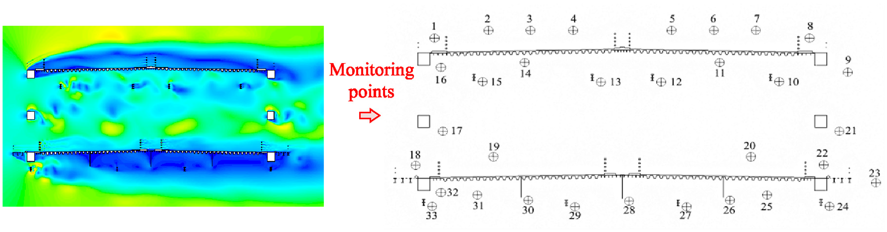
The contour of instantaneous velocities and the arrangement of monitoring points.

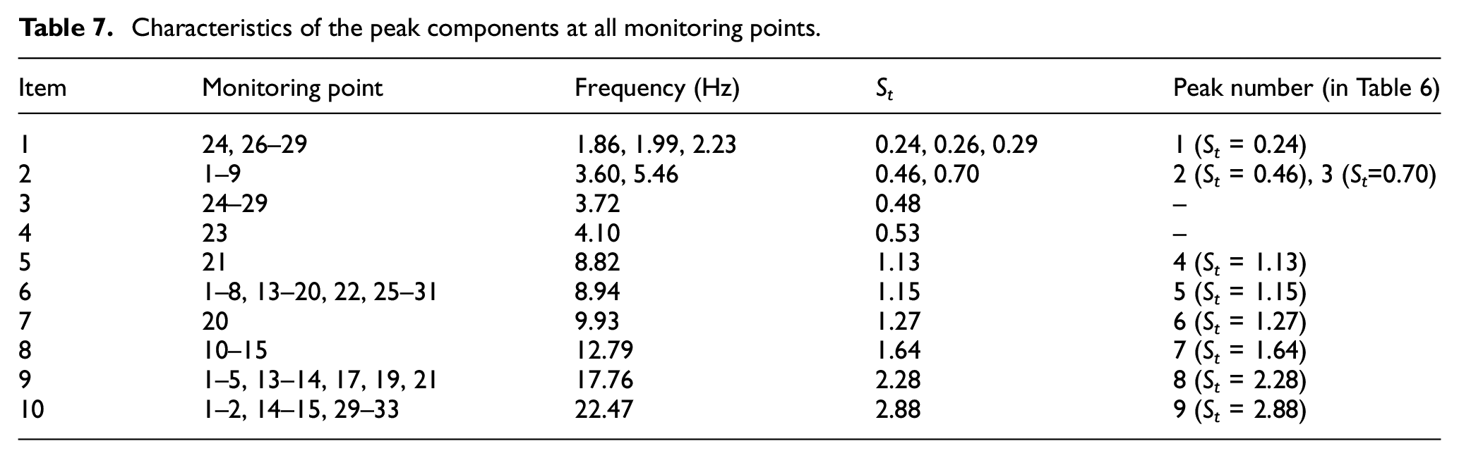
The time series of the wind velocities at the monitoring points were recorded and analyzed in the frequency domain. Their frequencies and the corresponding S_t numbers are shown in Table 7. It can be seen that the frequencies corresponding to the nine peaks in Table 6 could be recorded at different monitoring points. Moreover, several frequencies not obtained previously are recorded here. Then, the vortices driving the bridge to different VIVs are analyzed by comparing Tables 3 and 7. For the vertical VIVs of the bridge (S_t=0.41 and 0.7 in the wind tunnel tests), the similar results of 0.46 and 0.70 are recorded at P1-P9, that is, item 2 in Table 7, which indicates that the vibrations are probably driven by the shedding vortices above or behind the upper deck. For the major torsional VIV of the bridge at lower wind speeds (S_t=0.56 in the wind tunnel tests), the similar result of 0.53 is recorded at P23, that is, item 4 in Table 7, which indicates that the vibration is probably driven by the shedding vortices behind the service road. As P23 is located at the side of the truss girder, the shedding vortices are easier to drive the bridge to the torsional vibration. For the possible torsional VIV at higher wind speeds (S_t<0.31 in the wind tunnel tests), the possible results from 0.24 to 0.29 are recorded at P24 and P26-P29, that is, item 1 in Table 7, which indicates the vibration may be driven by the shedding vortices behind the vertical stabilizers.

Table 7.

Characteristics of the peak components at all monitoring points.

Item	Monitoring point	Frequency (Hz)	S_t	Peak number (in Table 6)
1	24, 26–29	1.86, 1.99, 2.23	0.24, 0.26, 0.29	1 (S_t = 0.24)
2	1–9	3.60, 5.46	0.46, 0.70	2 (S_t = 0.46), 3 (S_t=0.70)
3	24–29	3.72	0.48	–
4	23	4.10	0.53	–
5	21	8.82	1.13	4 (S_t = 1.13)
6	1–8, 13–20, 22, 25–31	8.94	1.15	5 (S_t = 1.15)
7	20	9.93	1.27	6 (S_t = 1.27)
8	10–15	12.79	1.64	7 (S_t = 1.64)
9	1–5, 13–14, 17, 19, 21	17.76	2.28	8 (S_t = 2.28)
10	1–2, 14–15, 29–33	22.47	2.88	9 (S_t = 2.88)

It should be noted that these peak components may be caused by the presence of more than one vortex migrating across the width direction of the decks. The following analysis will focus on the major torsional VIV which is significant in the wind tunnel tests at lower wind speeds. As the similar dominant frequency is only recorded at P23, the local region (see Figure 10) was focused to better understand the generation of the vortices. The vorticity contours at six different times within a vortex shedding period T are shown in Figure 13. When passing through the leeside service road, a part of winds above the lower deck flow into the gaps between the longitudinal beams and forms several vortices, while the rest forms another vortex at the tail of the service road. As the vortices fill up the gaps, the wind pressure below the service road increases gradually. When the wind pressure at the lower side of the service road is larger than the upper side, the winds flow out from the gaps and converge into the tail vortex. Meanwhile, the tail vortex becomes stronger and stronger, and it eventually separates from the girder and moves toward P23. This single vortex is formed alternately at the tail of the service road, which may produce fluctuated aerodynamic forces on the girder and drive the bridge to vibrate when the fluctuated frequency is close to the structural torsional frequencies.

Figure 13.

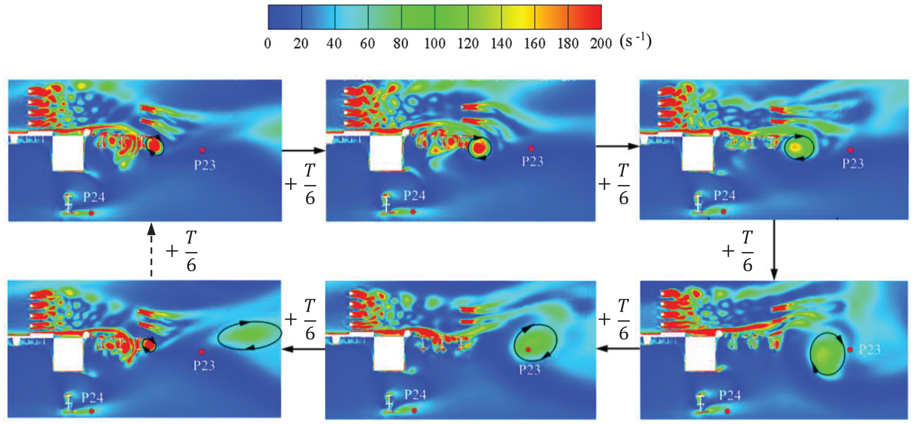
Vorticity contours at the tail of the service road within a vortex shedding period.

Further discussions on the single alternate vortex

In this section, the effects of different wind velocities and different positions of the diagonal bracing members on the single alternate vortex at the tail of the service road which may drive the bridge to the significant torsional VIV are investigated.

First, the computed wind velocity of the incoming flow was increased to 8 and 14 m/s, respectively, to study the effect on the single alternate vortex at the tail of the service road. For different cases, the wind velocity at P23 was recorded. The time series of the wind velocity are analyzed in the frequency domain, and the amplitude spectrums are shown in Figure 14. It can be seen that the dominant component becomes more prominent as its amplitude increases. The dominant frequency increases with the increase in wind velocity of the incoming flow, but S_t keeps unchanged, that is, 0.53, 0.53, and 0.52 corresponding to the computed wind velocities of 5, 8, and 14 m/s, respectively.

Figure 14.

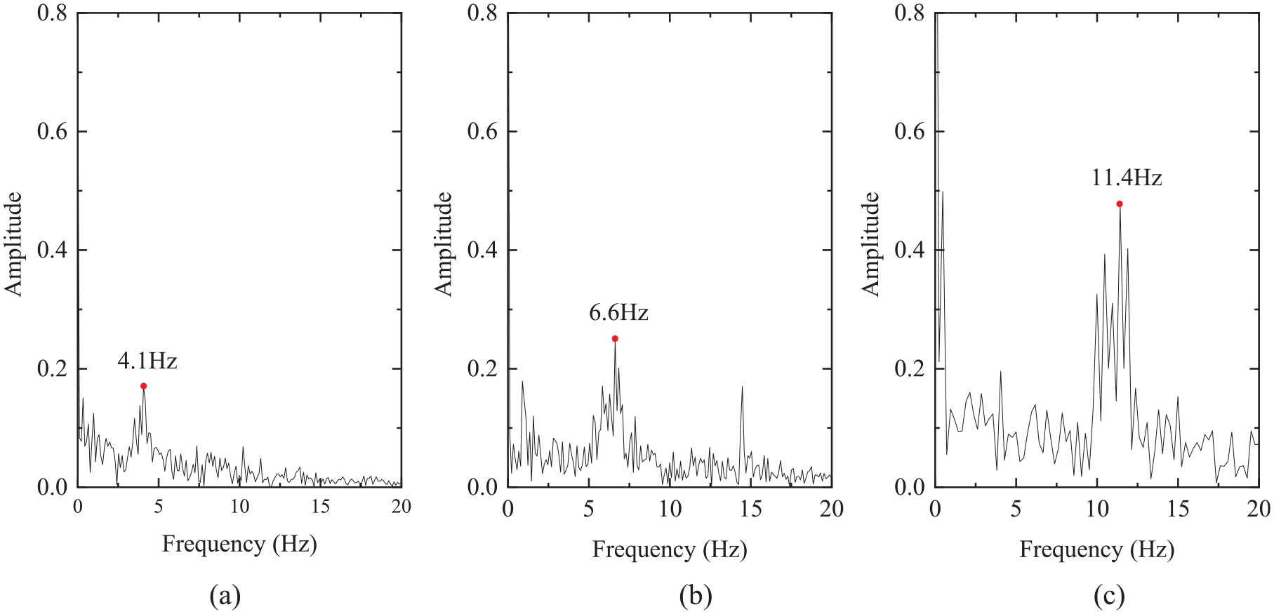
Amplitude spectrums of the wind velocity at P23 with different computed wind velocities: (a) 5 m/s, (b) 8 m/s, and (c) 14 m/s.

Subsequently, cross sections 1-1 and 3-3 were taken into account to fully describe the vortex shedding characteristics of the girder. The computational domains and parameters were the same as those for the previous case, and the computed wind velocity was set to 5 m/s. The time series of the wind velocity at P23 are analyzed in the frequency domain, and the amplitude spectrums are shown in Figure 15. It can be seen that the changes in the diagonal bracing members have certain effects on the vortex at the tail of the service road. Compared with the peak component for cross section 2-2, more peak components with similar frequencies could be observed in the amplitude spectrums for cross sections 1-1 and 3-3.

Figure 15.

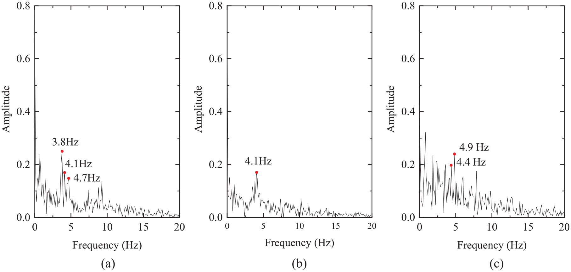
Amplitude spectrums of the wind velocity at P23 with different cross sections: (a) cross section 1-1, (b) cross section 2-2, and (c) cross section 3-3.

Conclusion

This paper studies the vortex-induced vibration performance of a truss girder with two decks based on the wind tunnel tests and the numerical simulations. Main conclusions can be drawn as follows.

(1) Vortex-induced vibrations of this type of truss girders are likely to occur. Several lock-in regions with the same frequency were observed in the wind tunnel tests. At three tested angles of attack, the major lock-in ranges with larger amplitudes are almost the same, while the minor lock-in ranges with smaller amplitudes are different. The existence of the secondary elements plays an important role in the VIVs.

(2) CFD simulations are then carried out to understand the reason driving the bridge to the VIVs. As the truss girder consists of many members, various vortices with different dominant frequencies are formed in the wake flow. The vertical VIV of the bridge is probably driven by the vortices behind or above the upper deck, which is related to the guardrails. The torsional VIV of the bridge is probably driven by the vortices behind or below the lower deck, which is related to the service road at lower wind speeds while may be related the vertical stabilizers at higher wind speeds.

(3) The vortex at the tail of the service road is one of the probable reasons driving the truss girder to the torsional VIV when the shedding frequency of the vortex is close to the natural torsional frequencies of the bridge. Based on the understanding of the flow field, the vortex could be weakened by optimizing the service road and the firefighting pipe, while the effectiveness should be validated.

(4) This paper focuses the VIV performance of the truss girder and the probable aerodynamic mechanism, while the optimization measures on the VIV need to be further investigated. To fully consider the aerodynamic interference among the truss members, 3D CFD simulations should be performed, considering the effects of angles of attack with various wind speeds systematically.

Footnotes

Declaration of conflicting interests

The author(s) declared no potential conflicts of interest with respect to the research, authorship, and/or publication of this article.

Funding

The author(s) disclosed receipt of the following financial support for the research, authorship, and/or publication of this article: The authors are grateful for the financial supports from the National Natural Science Foundation of China (Grants 51708463, 51525804) and the Fundamental Research Funds for the Central Universities (2682019CX04).

ORCID iDs

Ruijie Hu

Haojun Tang

References

Battista

Pfeil

(2020) Reduction of vortex-induced oscillations of Rio–Niterói bridge by dynamic control devices. Journal of Wind Engineering and Industrial Aerodynamics 84(3): 273–288.

Chen

Liu

, et al. (2017) Experimental investigations on VIV of bridge deck sections: A case study. KSCE Journal of Civil Engineering 21(7): 2821–2827.

Corriols

Morgenthal

(2012) Computational analysis of VIV observed on existing bridges. In: The seventh international colloquium on bluff body aerodynamics and applications (BBAA7), Shanghai, China, 2–6 September 2012.

De Miranda

Patruno

Ricci

, et al. (2015) Numerical study of a twin box bridge deck with increasing gap ratio by using rans and les approaches. Engineering Structures 99: 546–558.

Deniz

Staubli

(1997) Oscillating rectangular and octagonal profiles: Interaction of leading-and trailing-edge vortex formation. Journal of Fluids and Structures 11(1): 3–31.

Fujino

Yoshida

(2002) Wind-induced vibration and control of trans-Tokyo bay crossing bridge. Journal of Structural Engineering 128(8): 1012–1025.

Hourigan

Thompson

Tan

(2001) Self-sustained oscillations in flows around long blunt plates. Journal of Fluids and Structures 15: 387–398.

Larsen

(1995) A generalized model for assessment of vortex-induced vibrations of flexible structures. Journal of Wind Engineering and Industrial Aerodynamics 57(2): 281–294.

Larsen

Esdahl

Andersen

, et al. (2000) Storebælt suspension bridge – Vortex shedding excitation and mitigation by guide vanes. Journal of Wind Engineering and Industrial Aerodynamics 88(2): 283–296.

10.

Laima

, et al. (2011) Investigation of vortex-induced vibration of a suspension bridge with two separated steel box girders based on field measurements. Engineering Structures 33(6): 1894–1907.

11.

Tang

, et al. (2018a) Flutter performance optimization of steel truss girder with double-decks by wind tunnel tests. Advances in Structural Engineering 21(6): 906–917.

12.

Zhou

Liao

, et al. (2018b) Numerical studies of the suppression of vortex-induced vibrations of twin box girders by central grids. Wind and Structures 26(5): 305–315.

13.

Wang

, et al. (2018) Vortex-induced vibration performance and suppression mechanism for a long suspension bridge with wide twin-box girder. Journal of Structural Engineering 144(11): 04018202.

14.

Macdonald

JHG

Irwin

Fletcher

(2002) Vortex-induced vibrations of the Second Severn Crossing cable-stayed bridge: Full-scale and wind tunnel measurements. Structures and Buildings 152(2): 123–134.

15.

Mashnad

Jones

(2014) A model for vortex-induced vibration analysis of long-span bridges. Journal of Wind Engineering and Industrial Aerodynamics 134: 96–108.

16.

Nagao

Utsunomiya

Yoshioka

, et al. (1997) Effects of handrails on separated shear flow and vortex-induced oscillation. Journal of Wind Engineering and Industrial Aerodynamics 69–71: 819–827.

17.

Nakamura

Nakashima

(1986) Vortex excitation of prisms with elongated rectangular H and T cross-sections. Journal of Fluid Mechanics 163: 149–169.

18.

Naudascher

Wang

(1993) Flow-induced vibrations of prismatic bodies and grids of prisms. Journal of Fluids and Structures 7(4): 341–373.

19.

Seo

Lee

, et al. (2018) Prediction of wind velocity to raise vortex-induced vibration through a road-rail bridge with truss-shaped girder. Shock and Vibration 2018: 2829640.

20.

Owen

Vann

Davies

, et al. (1996) The prototype testing of Kessock Bridge: Response to vortex shedding. Journal of Wind Engineering and Industrial Aerodynamics 60: 91–108.

21.

Smith

(1980) Wind induced dynamic response of the Wye bridge. Engineering Structures 2(4): 202–208.

22.

Tang

Shum

, et al. (2020) Non-uniform wind characteristics in mountainous areas and effects on flutter performance of a long-span suspension bridge. Journal of Wind Engineering and Industrial Aerodynamics 201: 104177.

23.

Tang

Wang

, et al. (2017) Aerodynamic optimization for flutter performance of steel truss stiffening girder at large angles of attack. Journal of Wind Engineering and Industrial Aerodynamics 168: 260–270.

24.

Tang

Shum

Tao

, et al. (2019) Vortex-induced vibration of a truss girder with high vertical stabilizers. Advances in Structural Engineering 22(4): 948–959.

25.

Wang

, et al. (2019) Experimental and numerical studies of the vortex-induced vibration behavior of an asymmetrical composite beam bridge. Advances in Structural Engineering 22(10): 2236–2249.

26.

Zhu

(2015) Feasibility investigation on prediction of vortex shedding of flat box girder based on 2D RANS model. China Journal of Highway and Transport 28(6): 24–33 (in Chinese).