System fragility evaluation of a curved highway bridge structure considering multi-direction seismic excitations

Abstract

This paper presents the impact of varying the input seismic excitation directions on the system fragility of a geometrically complex highway bridge structure. The traditional approach of fragility derivation in the principal loading directions (longitudinal and transverse) results in an under/overestimation of the system fragility. To reduce such errors, the contribution of all major vulnerable components to the system fragility in the critical loading direction must be considered. For this purpose, a series of nonlinear time-history analyses were conducted for a testbed configured geometrically curved highway bridge structure in Japan. Shear strain, ductility, and distortion strain were considered as engineering demand parameters for bearings, concrete pier, and steel piers, respectively. The demand dependency among the components was considered using the correlation coefficient matrix for fragility estimation. Subsequently, fragility functions with respect to the input loading directions were generated for the bridge components and system to quantify their sensitivity to seismic input excitation directions. The results show that the component fragility is significantly influenced by the input excitation direction. A relative comparison of the system fragility for different loading directions indicated that a 150° loading direction yielded a higher fragility demand. The findings suggest that the critical fragility assessment should not always be decided only along the principal loading directions.

Keywords

seismic excitation directions system fragility curved bridge seismic isolation bearing probabilistic seismic demand models seismic input uncertainty

Introduction

Bridges are crucial links in road transportation networks and must remain serviceable during high-intensity seismic events. Previous seismic events have exposed the susceptibility of highway bridge structures to damages, which often result in high economic losses (e.g., Kobe earthquake in 1995, Chi-Chi earthquake in 1999, Wenchuan earthquake in 2008, Great East Japan earthquake in 2011, Guanshan and Chihshang earthquakes in Taiwan in 2022). Such events demonstrate the need for a seismic performance assessment (Basöz et al., 1999; Yamazaki et al., 2000). Horizontally curved bridges are usually installed at critical locations to cope with traffic congestion, topographical or structural limitations, and for aesthetic purposes. Owing to the horizontal curvature, the bending-torsion coupling interaction in the components that are subjected to asymmetrical loading results in a higher stress and deformation demand when compared to that of geometrically straight bridges (AmiriHormozaki et al., 2015; Falamarz-Sheikhabadi and Zerva, 2017). During the Petrolia seismic event of 1992, the South Fork Eel River Bridge experienced severe buckling resulting in fractures in its supporting frame and in-hinge connections (Itani et al., 2012). Similarly, during the Wenchuan earthquake of 2008, several curved spans of the Baihua Bridge collapsed (Yashinsky, 2009). Because of the curvature, the columns underwent larger displacements, which resulted in the unseating of girders. The dynamic performance of bridges under deterministic seismic excitations was studied using shaking table tests and parametric analysis to better understand the mechanical characteristics of horizontally curved bridges, which provide guidelines for seismic design (Li et al., 2015; Linzell and Nadakuditi, 2011; Williams and Godden, 1979; Wu and Najjar, 2007). However, seismic events are associated with high levels of uncertainties; therefore, structural responses may vary when subjected to varying ground motions. In this regard, a probabilistic seismic performance evaluation framework is a useful method to account for different uncertainties and involves the development of fragility functions (Nielson, 2005).

Probabilistic seismic performance assessments of curved bridges have recently gained popularity owing to their widespread use in California (Abbasi et al., 2016; Jeon et al., 2016; Movaghati and Abdelnaby, 2016; Pahlavan et al., 2016; Rogers and Seo, 2017; Shirazi et al., 2018). These studies have predominantly evaluated the effects of different structural and geometrical parameters on the seismic fragility of curved bridges, where the curvature is a significant influencing factor. Abbasi et al. (2016) evaluated the sensitivity of the component and system fragility functions for different limit states due to the changes in the structural layout in the horizontal and vertical planes. Another study reported pier height to be the most significant factor affecting component and system fragility (Jeon et al., 2016). Rogero and Seo (2017) ranked the span length, span width, and stiffness of supporting piers, which cause substantial variations in the seismic fragility of curved bridges. Kaleybar and Tehrani (2021) investigated the effect of different types of irregularities on the seismic behavior of curved reinforced concrete (RC) bridges in comparison to that of straight bridges. They reported significant differences in elastic and inelastic responses, particularly in the transverse direction, for varying combinations of pier height and abutment conditions. Apart from these findings, further studies have investigated the sensitivity of the seismic fragility of curved bridges to other factors such as nonlinear simulation and seismic characteristics using analytical models. Movaghati and Abdelnaby (2016) demonstrated that a calibrated fiber-based numerical model enables a more accurate fragility assessment by predicting the nonlinearity intrinsic to horizontally curved bridges under significant levels of multi-force interactions. According to Shirazi et al. (2018), the fragility curves of horizontally curved bridges are significantly influenced by the spectral characteristics of seismic waveforms and ground conditions. Therefore, seismic records with similar characteristics should be employed to avoid substantial underestimation of seismic fragility.

While previous research has primarily focused on the implications of structural geometrical factors, seismic characteristics, and numerical modeling techniques for the seismic fragility evaluation of geometrically curved bridges, the influence of the seismic excitation direction has rarely been considered. Previous studies have reported that the critical seismic behavior of buildings is strongly influenced by the orientation of the seismic excitation (Skoulidou and Romão, 2016). Several studies have investigated the effect of the loading direction on the dynamic characteristics of geometrically straight bridge structures. Torbol et al. (2012) and Basu and Shinozuka (2011) highlighted the importance of considering the effect of the incidence angle in the seismic fragility assessment of bridge structures and concluded that neglecting this parameter may lead to an underestimation of the resultant fragility functions. Similarly, Taskari et al. (2015) evaluated the multi-angle fragility of straight bridges and concluded that the fragility of individual components is highly sensitive to the input loading orientation. The seismic response of geometrically curved bridges is more complex because of the irregular distribution of mechanical characteristics, such as damping, stiffness, and strength, making them highly sensitive to the impact of the seismic-incidence orientation. However, there has been limited discussion on the development of the system fragility of geometrically irregular bridges with a specific focus on the effect of the seismic loading direction.

The objective of this study was to thoroughly investigate the system fragility of a geometrically curved bridge structure using a multicomponent approach, with a focus on comprehending the effects of ground motion directionality on the fragility profile. Initially, a finite element model was developed for a geometrically curved testbed bridge in Japan. Next, eigenvalue analysis was conducted to characterize the structural dynamics in terms of the resonant frequencies, dominant mode, and superstructure response. Subsequently, the global system fragility was evaluated in multiple loading directions based on the component fragility, while considering the correlation dependency between various components. Finally, variations in the components and system fragility profile were evaluated in terms of the median peak ground acceleration (PGA) values for varying input incidence directions. The findings of this study are expected to be of great significance to bridge systems with irregular geometries and complex dynamic characteristics.

Characteristics of the target bridge structure

Geometrical and structural properties

The target bridge in this study is a highway bridge in Japan. The total span of the bridge is 327.9 m and the width is 13–16.95 m for the mainline and 5.2–5.4 m for the ramps. It is a composite system consisting of steel and RC piers. The geometric complexities are due to the presence of on-off ramps and a horizontal curvature in the mainline. The total length is divided into six unequal spans that are supported by five steel and one RC pier, with abutment at the ends. Gate-shaped piers consisting of twin piers are provided in the wider zones, where the ramps join the main structure. The bridge stands on soil type II, which is a hard soil with a predominant period of 0.2 < Tg < 0.4 s.

The characteristic strengths of the concrete used in the superstructure and substructure are 30 and 24 N/mm², respectively. Throughout the structure, SM 490 (yield stress,

σ_{y} = 355 M P a

, Young’s modulus,

E = 206 G P a

, and Poisson’s ratio,

υ = 0.3

) and SS 400 (

σ_{y} = 235 M P a, E = 200 G P a, υ = 0.3

) steel framing sections are employed, which are super-heavy steel plates that are used for welded structures of bridges in highway construction. Lead rubber bearings (LRBs) are provided at the top of piers for seismic isolation. The geometric and structural details are listed in Table 1.

Table 1.

Geometrical and structural characteristics of the target bridge.

Properties	Pier 6	Pier 7	Pier 8	Pier 9	Pier 10	Pier 11
Height ( $m m$ )	9600	7850	10,850	11547L^, 12050R^*	9774L, 10300R	6150
Pier cross section ( $m m^{2}$ )	$\begin{array}{c} 4500 \\ \times \\ 3600 \end{array}$	$\begin{array}{c} 2000 \\ \times \\ 2000 \end{array}$	$\begin{array}{c} 2000 \\ \times \\ 2000 \end{array}$	$\begin{array}{c} 2000 \\ \times \\ 1500 \end{array}$	$\begin{array}{c} 2000 \\ \times \\ 1200 \end{array}$	$\begin{array}{c} 2000 \\ \times \\ 2000 \end{array}$
Pier cap dimension ( $m m^{2}$ )	$\begin{array}{c} 11800 \\ \times \\ 3600 \end{array}$	$\begin{array}{c} 13400 \\ \times \\ 2000 \end{array}$	$\begin{array}{c} 15800 \\ \times \\ 2000 \end{array}$	$\begin{array}{c} 22500 \\ \times \\ 2000 \end{array}$	$\begin{array}{c} 13350 \\ \times \\ 2000 \end{array}$	$\begin{array}{c} 11200 \\ \times \\ 2000 \end{array}$
Concrete infilled height ( $m m$ )	--	3850	5310	6050L, 5550R	5200L, 5500R	4450
Concrete/Steel E ( $k N / m m^{2}$ )	25	2 x 10⁵
Bearing cross section ( $m m^{2}$ )	$\begin{array}{c} 850 \\ \times \\ 850 \end{array}$	$\begin{array}{c} 1100 \\ \times \\ 1100 \end{array}$	$\begin{array}{c} 1100 \\ \times \\ 1100 \end{array}$	$\begin{array}{c} 950 \\ \times \\ 950 \end{array}$	$\begin{array}{c} 950 \\ \times \\ 950 \end{array}$	$\begin{array}{c} 950 \\ \times \\ 950 \end{array}$
Bearing thickness ( $m m$ )	217	186	186	216	220	192
Diameter of a lead plug ( $m m$ )	130	165	165	145	145	145
Number of lead plugs	4
Shear modulus G ( $N / m m^{2}$ )	1

*Left pier, ** right pier.

Finite element modeling

Because the bridge structure is curved with an on-off ramp, 3D analytical modeling was considered in this study, which was performed using the nonlinear analysis program Engineer’s Studio. The finite element model of the bridge and material constitutive models are shown in Figure 1. The bridge system was approximated using the frame and spring elements with discrete degrees of freedom. The lumped mass of the system was divided into several point masses at each discrete node throughout the sub- and superstructures. A bilinear stress–strain relationship with a strain-hardening slope of E/100 and kinematic hardening behavior was assumed for the steel sections, while a parabolic model was assumed for the concrete modeling, with a compressive strength equivalent to 0.85 times the design strength.

Figure 1.

Numerical model of the target bridge structure.

Superstructure, pier cap, abutments, and footing

The superstructure was modeled as a linear beam element that remains elastic under dynamic loading. Because the response is predominantly governed by isolation devices, the stiffness of the superstructure has no significant effect on the overall seismicity of the structure (Ghobarah, 1988). From a structural design perspective, piers can enter the inelastic range within allowable limits. Therefore, in active seismic regions, the inelastic behavior of piers must be considered in the analysis. Steel piers are partially filled with concrete and modeled as fiber elements, such that each fiber exhibits a stress–strain material model. The fiber elements were defined to confine the steel and concrete. The concrete pier was appropriately detailed according to the design requirements of the Japan Road Association (JRA) (JRA, 2002). Plasticization is expected to occur in the plastic hinge zone near the base of the concrete pier; therefore, nonlinearity was considered in the modeling using the nonlinear Takeda model. The bent-top beams were modeled as linear elastic beam elements. The material constitutive models were defined and section discretization was performed. For soil-structure interaction, six linear springs (three translational and three rotational springs) were defined to represent the foundations based on the mechanical characteristics of the soil types (JRA, 2002).

Isolation bearings and multi-shear spring model

Bridges are isolated by LRBs, which are widely employed worldwide owing to their high damping characteristics. The mechanical characteristics of these devices are influenced by their elastoplastic behaviors, compounding effect, and viscous properties due to temperature and strain rate (Abe et al., 2004; Bhuiyan et al., 2009). The mechanical response of the bearings can be characterized by the stiffness in relation to the strain rate, such that the initial stiffness is significantly high at a low strain rate. With an increase in the strain rate, the stiffness becomes constant and finally increases again in the strain-hardening stage. The mechanical response is represented using a bilinear model, where the relative drop in the post-yield stiffness (K₂) can be calculated using equation (1). The characteristic parameters of the bearings at different locations are listed in Table 2.

K_{1} = 6.5 K_{2}

(1)

Table 2.

Characteristics of the isolation bearings.

Properties	Pier 6	Pier 7	Pier 8	Pier 9	Pier 10	Pier 11
Pre-yield stiffness K1 (kN/m)	24,233	49,269	54,778	36,858	36,683	30,775
Characteristic strength Qd (kN)	442,636	713,062	713,062	455,400	550,675	550,675
Yield displacement (m)	0.0216	0.0171	0.0154	0.0146	0.0193	0.0211
Damping ratio h_b (%)	27.7	27.6	27.8	27.5	27.8	27.6

Additionally, because the direction of the bridge continuously changes in the horizontal plane, the bearings are represented by multi-shear spring (MSS) elements such that they show the same nonlinear characteristics throughout the horizontal plane (Wada and Hirose, 1989). The MSS model comprises a set of similar unidirectional spring elements, each with a bilinear constitutive model, whose parameters are calculated using the following equations.

k_{s} = \frac{k_{s}}{\sum_{i = 0}^{m - 1} \cos^{2} (\frac{i π}{m})}

(2)

q_{y} = \frac{Q_{y}}{\sum_{i = 0}^{m - 1} \cos^{2} (\frac{i π}{m})}

(3)

Here, k_s and K_s represent the stiffness values of a single spring and the overall MSS system, respectively, and q_y and Q_y are the yield strengths of an individual spring and the entire MSS system, respectively. An increase in the number of individual springs results in a smooth hysteresis response, but with a high computational cost. In this study, 12 springs were combined to simulate the MSS model, as shown in the figure.

The ground motions that were considered for the dynamic characterization were obtained from the accelerograms recorded at the Japan Railway Takatori (JRT) station, that is, JRT-NS and JRT-EW components, as shown in Figure 2, which correspond to the longitudinal and transverse inputs, respectively, with PGAs of 0.70 and 0.68 g, respectively, as suggested by the JRA (JRA, 2002). These waveforms are the modified seismic records obtained from the 1995 Kobe earthquake, which are Level-II-type ground motions corresponding to Ground-type II, and are recommended in the design code (JRA, 2002). A two-step loading was adopted for the dynamic analysis, where the dead load was followed by a seismic motion input with an incremental time step of 0.01 s.

Figure 2.

Accelerograms for dynamic characterization (a) JRT-NS component (b) JRT-EW component.

An eigenvalue analysis was conducted to obtain basic insights into the dynamic properties of the bridge. The first few modal frequencies and corresponding effective mass ratios are listed in Table 3. The fundamental resonant mode was excited in the lateral direction with a frequency of 0.63 Hz, which falls within the generally accepted range of fundamental periods for multi-span bridges as described in the literature (Zelaschi et al., 2016). As shown in Figure 3, the first and second modes are radial and tangential, respectively. Most of the higher modes are dominated by the torsional response. Mode seven is a complex vertical-torsional vibration mode, where the deformation and twisting motions are amplified at the side abutments and mid-span of the structure, respectively.

Table 3.

Resonant frequencies and the associated modes.

Mode #	f (Hz)	T (s)	Effective mass ratio (%)			Type of mode
Mode #	f (Hz)	T (s)	Longitudinal	Vertical	Transverse	Type of mode
1	0.630	1.587	0.016	0.000	37.534	Radial
2	0.664	1.506	42.629	0.000	0.000	Tangential
3	0.694	1.441	0.478	0.000	1.062	Torsional
4	0.833	1.200	0.006	0.000	1.390	Torsional
5	1.158	0.864	0.013	0.000	0.813	Torsional
6	1.209	0.827	0.065	0.000	0.762	Torsional
7	1.450	0.690	0.046	0.043	0.117	Vertical +Torsion

Figure 3.

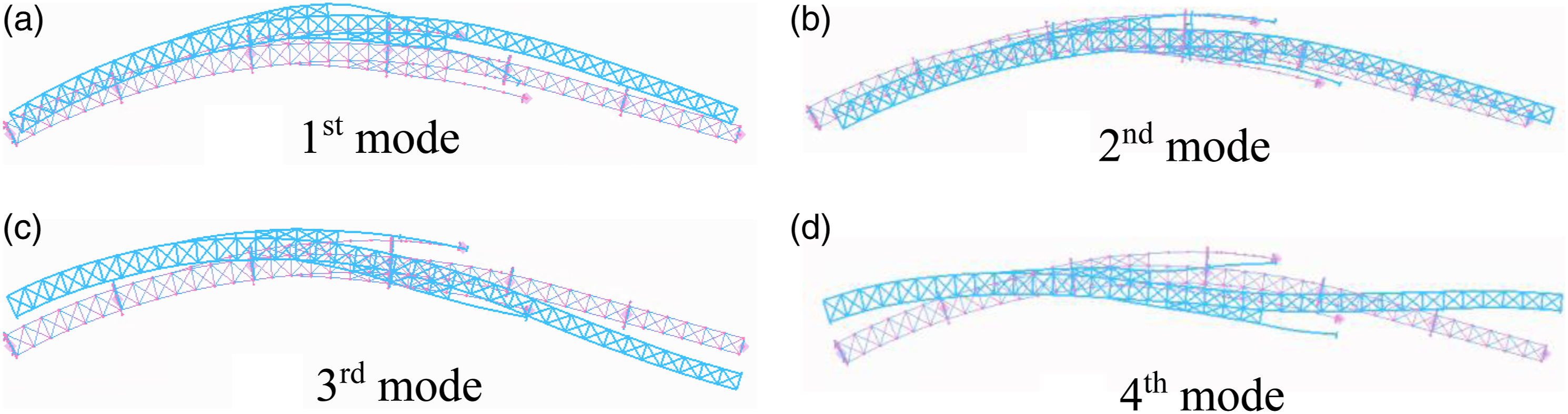
Predominant modal shapes: (a) Radial (b) Tangential (c) Torsional (d) Torsional.

Responses of the components

This section describes the inelastic behavior of steel piers and isolation bearings using a nonlinear time-history response analysis, considering the modified JRT waveforms in the orthogonal directions. The vertical excitation component is not considered here because of its insignificant effect on the seismic behavior of the bridge structure (Usami et al., 2004). Dussea et al. (1989) revealed that unequal dynamic excitation at the base of the structure significantly affects the dynamic characteristics of long-span bridges. However, because the target bridge has a comparatively shorter span, equal dynamic excitation was considered for all supports when performing the time-history analysis.

Figure 4 shows the displacement time history of the middle pier (Pier 8) and the associated bearing in the local (longitudinal and transverse) directions. A general comparison shows that the bearings are highly effective in reducing the displacement demand on the pier. The maximum longitudinal displacement of the bearing is 463.2 mm, which is more than three times the displacement of the pier. A similar response is observed in the transverse direction. The residual displacements in both cases are in the order of a few millimeters. The axial force time histories for the same pier are shown in Figure 5 in both directions in the local coordinate system, where the force is nondimensionalized by the squash load N_y of the section, which is 77,631 kN at the base of the pier. In the longitudinal and transverse directions, the compressive axial force under dead load is approximately 0.12N_y, which upon seismic excitation increases to a maximum of 0.137N_y and 0.143N_y, respectively. Thus, in conclusion, the earthquake excitation does not cause a significant increase in the axial force response. Steel members are typically susceptible to axial strain during compression, which ultimately contributes to buckling. The axial force demand was larger in the transverse loading direction; therefore, only the strain time history at the base of the pier is shown in Figure 6(a). The section deformations are of moderate magnitude, resulting in a peak strain of approximately 9.28 $ε_{y}$ . The hysteresis response of a typical bearing in the transverse direction is shown in Figure 6(b), where the bearing undergoes a maximum displacement of approximately 325 mm. The resulting shear strain was approximately 174.7%, which is lower than the strain corresponding to the ultimate failure as per the design recommendations (JRA, 2002).

Figure 4.

Displacement response history of the pier and bearing at P8 (a) Longitudinal direction (b) Transverse direction.

Figure 5.

Axial compressive force response at the base of P8 (a) Longitudinal excitation (b) Transverse excitation.

Figure 6.

Inelastic response of the steel pier and bearing at P8 (a) Strain response of steel pier (b) Hysteresis response of the bearing.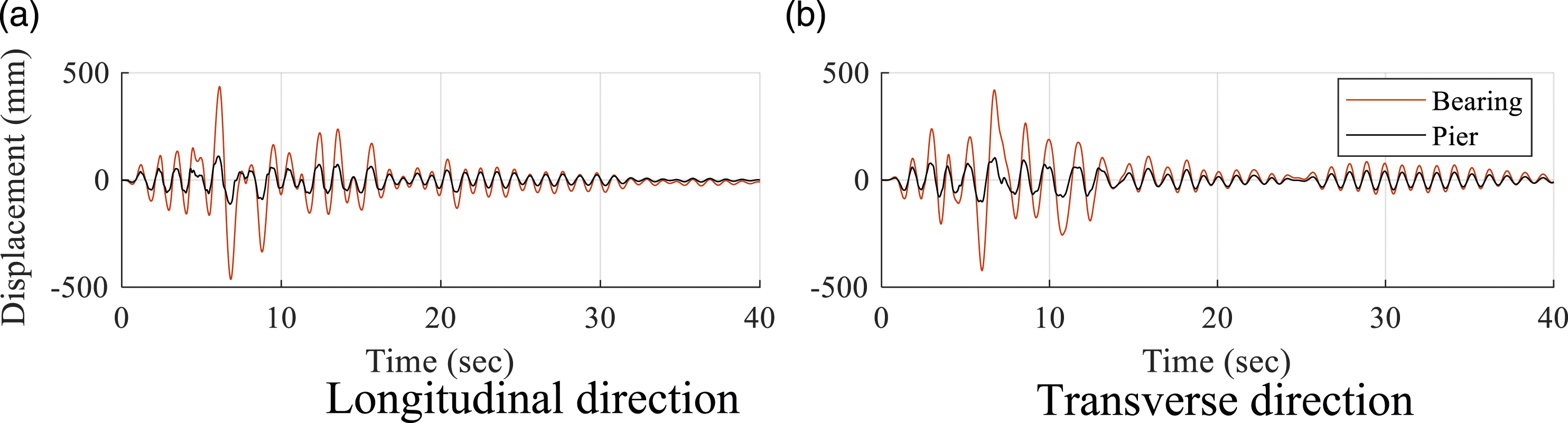

Analytical fragility functions

The fragility functions were derived using a probabilistic seismic demand model (PSDM), which was developed from the nonlinear time-history-based simulations. The PSDM relates the engineering demand parameter (EDP) with the demand intensity measure (IM). The derivation of a PSDM requires the selection of an appropriate IM, which results in a lower variation in the structural response. Different studies have employed different IMs for fragility derivation, such as the PGA, peak ground velocity (PGV), and spectral acceleration in the fundamental mode, as proposed in the literature. However, the PGA is acknowledged to be the most effective and optimal IM. Studies have suggested that the optimality of an IM is based on its efficiency (lower variation in the estimated demand), practicality (high correlation between the component response and ground motion), proficiency (composite measure of efficiency and practicality), sufficiency (measure of independence of other ground motion parameters for the given ground motion), and hazard computability (minimal effort to compute probabilistic seismic hazard) (Padgett et al., 2008). By using these parameters, Padgett et al. (2008) evaluated the seismic fragility of multi-span steel girder bridges considering 10 IMs and suggested PGA as the most appropriate IM for PSDM derivation. Another study evaluated the optimality of seven IMs for different structural components of cable-stayed bridges by considering synthetic and recorded ground motions (Zhong et al., 2019). The results revealed that PGA and PGV were the most optimal IMs for the short- and long-period structural components, respectively. Furthermore, several studies have considered the PGA in fragility estimation because of its overall efficiency, proficiency, practicality, sufficiency, and hazard computability (Billah et al., 2013; Billah and Alam, 2015).

A PSDM can be developed using a cloud (Choi et al., 2004; Nielson and DesRoches, 2007b; Padgett and DesRoches, 2008) or scaling approach (Zhang and Huo, 2009). In the cloud approach, the original unscaled ground motions are used in the simulations, and for each ground motion, the response is plotted against the IM after a time-history analysis. Conversely, in the scaling approach, each ground motion is scaled to a selected maximum value, and the analysis is performed using an incremental dynamic analysis (IDA) method. The IDA is helpful when the number of available ground motions is limited, thereby creating a reasonable set of data points for PSDM development. Each increment in the IDA involves a complete time-history analysis to capture the structural response at a particular IM value. The current study considers the scaling approach, where each accelerogram is scaled from 0.2 to 2g, thus creating an ensemble of 200 input records. Using the IDA, sufficient response data that correspond to various input IMs can be generated. Regression analysis was performed to estimate the PSDM for each component.

To formulate the fragility functions, a basic reliability-theory-based definition was considered. Accordingly, the fragility can be expressed by as follows:

P_{f} = P [\frac{S_{d}}{S_{c}} \geq 1]

(4)

where P_f is the component or system failure probability and S_d and S_c represent the seismic demand and structural capacity, respectively. The seismic demand and capacity were assumed to follow lognormal distributions. In lognormal space, equation (4) can be transformed as follows:

P_{f} = P [\ln \frac{S_{d}}{S_{c}} \geq \ln (1)] = P [\ln S_{d} - \ln S_{c} \geq 0]

(5)

As a lognormal distribution is assumed, the demand and capacity distributions can be represented as follows:

\begin{array}{l} \ln S_{d} : N (λ_{d}, β_{d}^{2}) \\ \ln S_{c} : N (λ_{c}, β_{c}^{2}) \end{array},

(6)

where λ is the mean and β is the standard deviation of the normal distribution. Using probability principles, the demand and capacity can be combined as shown below.

\ln S_{d} - \ln S_{c} : N (λ_{d} - λ_{c}, β_{d}^{2} + β_{c}^{2})

(7)

The seismic demand can be measured using an appropriate parameter known as the EDP, which can be related to the IM using the following power law.

E D P = S_{d} = a {(I M)}^{b}

(8)

Here, a and b are regression coefficients that can be estimated from the response data collected from the nonlinear time-history analysis. The demand dispersion conditioned on the IM can be computed as follows (Baker and Cornell, 2006):

β_{d} = \sqrt{\frac{\sum_{i = 1}^{N} {(\ln (D_{i}) - \ln (a {(I M)}^{b}))}^{2}}{N - 2}}

(9)

where Di is the achievement of component demand and N denotes the total number of analysis cases. To account for the uncertainty in the component capacity, each limit state can be associated with a coefficient of variation (COV), which can be calculated using equation (10) (Nielson, 2005). Then, the failure probability can be calculated using the relation in equation (11), which can be transformed into a generalized fragility expression as shown in equation (12).

β_{c} = \sqrt{\ln (1 + C O V^{2})}

(10)

P [L S | I M] = Φ (\frac{\ln (a I M^{b}) - \ln (S_{c})}{\sqrt{β_{d}^{2} + β_{c}^{2}}}) = Φ (\frac{\ln (I M) - (\frac{\ln (S c) - \ln (a)}{b})}{\frac{\sqrt{β_{d}^{2} + β_{c}^{2}}}{b}})

(11)

P [L S | I M] = Φ (\frac{\ln (I M) - \ln (λ)}{ξ})

(12)

Here, Φ [*] is the standard normal cumulative distribution function, λ and ξ are the mean and dispersion of the lognormal distribution describing the fragility functions.

Component fragility curves are useful for identifying the most vulnerable components and making retrofitting decisions. However, system (bridge) fragility curves are more convincing and essential for use in transportation-network seismic risk assessment platforms. Moreover, during seismic excitation, structural components experience different damage states, leading to a complex damage state of the bridge. Thus, the damage state of the bridge system cannot be expressed by any single-component damage state; therefore, the global system fragility must be evaluated to approximate the structural behavior (Choi et al., 2004; Mackie and Stojadinović, 2007; Nielson and DesRoches, 2007a; Zhang and Huo, 2009).

If component fragility curves are already available, system-wide fragility curves can be developed directly using these curves. Traditionally, a bridge system is considered a series system, for which system fragility can be expressed in terms of lower and upper bounds using reliability theory. Based on this theory, a single-component failure leads to the failure of the entire system. In this case, the global damage state of the system is considered based on the governing component response. Mathematically the fragility bounds of the system can be expressed as follows:

\max_{i = 1}^{m} [P (F_{i})] \leq P (F_{s y s}) \leq 1 - Π_{i = 1}^{m} [1 - P (F_{i})]

(13)

where P [Fi] and P [Fsys] denote the failure probabilities of component i and the system, respectively. Equation (13) suggests that the lower bound yields non-conservative estimates of system fragility, whereas the upper bound is more conservative.

In a real-world system, the actual fragility lies between these two extremes. To calculate the exact fragility curve, another alternative is using the joint PSDM (JPSDM) method combined with a Monte Carlo simulation (MCS), which considers the correlation dependency between different components (Nielson, 2005). First, using the MCS, N random demand samples are generated and compared with the capacity limit states. For a given IM, the failure probability of the system is calculated using equation (14), for which the failure samples are tracked using the indicator function I_F, as defined in equation (15).

P [F_{s y s} | I M] = \frac{\sum_{i = 1}^{N} {I_{F}}_{i}}{N}

(14)

I_{F} = {\begin{cases} 1 if (x_{1}, x_{2} . . . x_{n}) \in F_{1,2, . . ., n} \\ 0 if (x_{1}, x_{2} . . . x_{n}) \notin F_{1,2, . . ., n} \end{cases}

(15)

Here,

(x_{1}, x_{2} . . . x_{n})

represents the random demand sample and

F_{1,2, . . ., n}

is the failure domain defined by the capacity limit states of n components. In the current study, both methods were analyzed and compared in terms of median PGA values.

Ground motions selection and excitation direction

Fragility functions require the development of a relationship between the structural demand resulting from ground motion and the corresponding damage matrix. This can be performed either by collecting the actual seismic data and analyzing the damage statistics or by utilizing the representative physical model subjected to a set of ground motions. The former option is more reliable and realistic but is not useful when the data are deficient. In such cases, the latter method is considered, which results in well-distributed input-output pair of data from the analysis. However, the selection of ground motion for time-history analysis requires a great deal of care.

The structural response is highly dependent on the characteristics of the input waveform, which increases the uncertainty in the numerical analysis. For seismically active regions, the usual practice is to select recorded ground motions in the study area. Similarly, this study considers a suite of 20 representative ground motions, which were retrieved from strong ground motion databases such as the Japan Meteorological Agency (JMA), Kyoshin Network, and Kiban Kyoshin Network, having PGA values ranging from 0.18 to 2.49 g. These records correspond to level-II earthquakes, which have a low frequency of occurrence and are highly destructive. Vertical components were not considered because of their less significant impact on the structural performance (Abbasi et al., 2016; Mosqueda et al., 2004; Usami et al., 2004). However, for near-field ground motions, the impact of the vertical component may be statistically significant and should not be neglected, which is not the case in this study (Zhong et al., 2023). The characteristics of the selected waveforms are listed in Table 4. Figure 7(a) shows the acceleration response spectra of the recorded ground motions along with the different percentiles of the acceleration response spectra, which represent medium-to high-intensity accelerograms following the design guidelines (JRA, 2002). The statistical mean and 25th and 75th percentiles of acceleration response spectra with 5% damping ratio were calculated using the magnitude values of the response spectrum of all the selected waveforms at each incremental time period.

Table 4.

Characteristics of the selected ground motion records.

S. No	Earthquake name	Recording region	Year	Richter magnitude	PGA (g)
1	Iwate	Higashinaruse	2008	7.2	0.26
2	Iwate	Higashinaruse	2008	7.2	2.49
3	Tottori seibu	Hino	2000	6.7	0.59
4	Tottori seibu	Hino	2000	6.7	0.77
5	Iwate	Ichinoseki nishi	2008	7.2	0.76
6	Iwate	Ichinoseki nishi	2008	7.2	1.46
7	Kobe	JMA kobe	1995	7.2	0.63
8	Kobe	JMA kobe	1995	7.2	1.34
9	Niigata chuetsu	Kawaguchi	2004	6.8	1.71
10	Kumamoto	Mashiki	2016	7.0	0.25
11	Kumamoto	Mashiki	2016	7.0	0.94
12	Niigata chuetsu	Nagaoka	2004	6.8	0.32
13	Niigata chuetsu	Nagaoka	2004	6.8	0.67
14	Niigata chuetsu	Ojiya	2004	6.8	1.33
15	Kumamoto	Otsu	2016	7.0	0.49
16	Kumamoto	Shougoku	2016	7.0	0.18
17	Kumamoto	Shougoku	2016	7.0	0.67
18	Niigata chuetsu	Tokamachi	2004	6.8	0.86
19	Hokkaido tokachi	Taiki	2003	8.3	0.35
20	Hokkaido tokachi	Tsurui higashi	2003	8.3	0.32

Figure 7.

Selected accelerograms and applied loading directions (a) Acceleration response spectra of the selected waveforms with different percentiles (b) Waveform loading direction (in degrees) w.r.t Pier 9.

Typically, for geometrically straight bridges, seismic loads are applied in the longitudinal and transverse directions. In such cases, the transverse direction is considered to be more vulnerable, and the fragility of the system is determined based on this direction. To understand how the direction of ground motion affects the vulnerability of a curved bridge, horizontal components were applied along the X-axis and then gradually rotated around the Z-axis by a certain angle. In this study, rotation was conducted for the interval $0^{\circ} \leq θ \leq 150^{\circ}$ at incremental angles of 30°, as shown in Figure 7(b).

Limit states

Usually, for seismically isolated continuous composite bridge systems, isolation bearings and piers are the most critical components, which are often forced to enter a nonlinear range during seismic events. The damage behaviors of these components are measured using the appropriate EDPs. Post-earthquake reports have predominantly indicated that column damage and bearing failures are the most common types of failures for typical bridges (Zhong et al., 2015). In the current study, LRBs, concrete piers, and steel piers were considered as critical components. Accordingly, shear strain, displacement ductility, and distortion strain were used as the EDPs for LRBs, concrete piers, and steel piers, respectively. For the component damage assessment, the capacity models must be defined in terms of the same unit as the EDP (Nielson, 2005). Based on the qualitative damage criteria of the HAZUS Earthquake Model, four damage states were considered in the performance assessment (HAZUS-MH, 2012). The details of the various damage states are summarized in Table 5. The limit states of the bearings were based on experimental observations and considerations of the secondary effects of unseating and pounding at the abutments. Typically, the EDPs considered for isolation bearings are shear strain and displacement. The dimensionless shear strain parameter is more convenient in cases where a variation exists in the dimensions of the bearings. LRBs undergo different mechanical behaviors with an increase in demand (Abe et al., 2004). The bearings exhibit stiffness variation, which is significantly high at very-low strain demands, becoming constant at low to medium strain levels, and finally becoming significantly high, corresponding to the strain-hardening stage at high strain demands. Modern isolation devices are capable of enduring a shear strain of up to 400% before an ultimate capacity loss. Such large straining may result in the undesirable effects of pounding at the abutment and a larger lateral displacement of the superstructure. Therefore, complete damage is defined as the verge of reaching a strain of 250% (JRA, 2002). For the steel piers, the damage states were based on the design documentation. The EDP collectively considers the effects of axial and bending deformations. A slight damage state corresponds to the yielding strain, whereas a collapsed damage state is defined at the ultimate strain level.

Table 5.

Definition of the limit states of components.

Component	Damage state	Slight	Moderate	Extensive	Collapse	Source
	Failure mode	Spalling	Moderate cracking	Moderate crushing	Severe crushing	(HAZUS-MH, 2012)
Concrete pier	Displacement ductility	$μ_{d} > 1$	$μ_{d} > 1.2$	$μ_{d} > 1.76$	$μ_{d} > 4.76$	(Hwang et al., 2001)
LRB	Shear strain (%)	$γ > 100$	$γ > 150$	$γ > 200$	$γ > 250$	(Zhang and Huo, 2009)
Steel pier	Distortion (%)	$ε_{y}$	--	--	$7 \times ε_{y}$	*

*Bridge design document.

Resultant fragility curves and discussion

The selected waveforms were applied in multiple directions, and for each direction, the fragility functions were derived using equation (12). Initially, the PSDMs were developed for each component using the IDA results by correlating the IM demand with the corresponding component EDPs. Each accelerogram was scaled with an equal increment of 0.2 g to a maximum of 2.0 g. This way a total of 200 nonlinear time-history analyses were conducted for each loading direction.

Probabilistic seismic demand models (PSDMs) for bridge components

The PSDMs were generated for the selected components in different excitation directions using equation (8). Notably, the seismic demand for structural components varies as a function of the input loading direction. The differences in the structural response revealed the differences in the structural resistance for various loading incidence directions. The structural resistance is primarily related to the stiffness of the components, which, in turn, is based on the geometric configuration of a particular component. Therefore, the governing component for the fragility estimation varies. Unlike the steel piers, the bearings showed higher sensitivity to the input loading direction, as shown in Table 6. For example, in the 0° loading direction, in addition to the concrete (Pier 6) and steel pier (Pier 8), the most fragile bearing was the bearing at the top of Pier 6. Similarly, in the 30° and 60° loading cases, the bearings at Piers 11 and nine were to be the most fragile, respectively. Because system fragility is defined based on the most fragile components in each loading direction, the PSDMs are considered for the governing components in each loading direction. Table 7 presents the median expression for the PSDMs and the dispersion for the selected components that are transformed into logarithmic space. Notably, the PSDM for each component varies with the changes in the input loading direction. The dispersion estimates did not vary significantly and were less sensitive to the loading direction for the curved bridge examples.

Table 6.

Location of most critical bearings with respect to loading direction.

Loading direction	0°	30°	60°	90°	120°	150°
Critical bearing location (top of pier)	Pier 6	Pier 11	Pier 9	Pier 9	Pier 9	Pier 6

Table 7.

Probabilistic seismic demand models for different components in different loading directions.

Loading direction	Response	Ln (γ)	Ln (μd)	Ln (ϵ)
0°	PSDM	1.02×ln (PGA)+2.07	1.01×ln (PGA)+0.96	0.87×ln (PGA)-0.06
0°	βd	0.67	0.60	0.87
30°	PSDM	1.13×ln (PGA)+1.95	0.97×ln (PGA)+0.63	0.88×ln (PGA)+0.02
30°	βd	0.70	0.57	0.87
60°	PSDM	1.04×ln (PGA)+1.82	1.16×ln (PGA)+0.83	0.85×ln (PGA)+0.21
60°	βd	0.63	0.65	0.84
90°	PSDM	1.06×ln (PGA)+1.92	1.15×ln (PGA)+0.81	0.83×ln (PGA)+0.13
90°	βd	0.64	0.63	0.84
120°	PSDM	1.09×ln (PGA)+2.09	0.98×ln (PGA)+0.59	0.89×ln (PGA)+0.21
120°	βd	0.68	0.57	0.87
150°	PSDM	1.03×ln (PGA)+2.14	1.02×ln (PGA)+0.90	0.89×ln (PGA)+0.08
150°	βd	0.66	0.59	0.87

The variation in the median estimates of the PSDMs considering the loading direction can be reflected more directly using the polar diagrams, as shown in Figure 8. The radial coordinates represent the responses of the components in terms of their respective EDPs (ln (γ), ln (μd), and ln (ϵ)). Different components have different levels of dependence on the load-incidence direction. The sensitivity of the EDPs of the components to the excitation direction depends on the magnitude of the PGA value; that is, the demand with a lower PGA tends to be more dependent on the excitation directions. For example, in Figure 8(a), the maximum shear strain at PGA=0.1 and 0.5 g shows high fluctuation. For the bearings, the maximum shear strain appears at θ =150°. Concrete piers exhibit a comparatively high sensitivity to the load-incidence direction. This can be attributed to the anisotropic mechanical properties of the rectangular section in all directions. The maximum curvature ductility ratio attains the maximum value of 6.62 at θ =90° (e^1.89=6.62 from Figure 8(b)). Although steel piers yield lower EDP results even at higher demand values, the effect of load-incidence angle is noticeable from Figure 8(c), where the minimum and maximum distortion strains appear at θ =0° and θ =120°, respectively.

Figure 8.

PSDMs for components in the 0^o loading direction (a) Rubber Bearing (b) Concrete Pier (c) Steel Pier.

Component fragility

The fragility curves were calculated from the respective PSDMs and limit state models using equation (12) for the bearing, concrete pier, and steel pier, as shown in Figure 9(a)–(c) for the 0° loading case. Component fragility is sensitive to the loading direction because the governing fragile components vary with changes in the loading direction. Therefore, for each component class, fragility curves were calculated based on the most vulnerable components for the respective limit states. From the results, it is obvious that the isolation bearings are the most vulnerable among the bridge components owing to the design requirements of the isolation bridge structure. The median probability of yielding state for the LRB, concrete pier, and steel pier were attained at 0.13, 0.39, and 1.06 g, respectively. This illustrates the likelihood that the components are vulnerable to a given input demand. Owing to the highly sophisticated seismic design of the steel piers, the failure probability was considerably lower in the respective damage states. For the concrete pier, the fragility in the slight, moderate, and extensive damage states was considerably higher than that in the collapsed state, showing higher susceptibility to cracking and spalling even in the lower demand range.

Figure 9.

Fragility curves in 0^o loading direction for bridge components (a) Isolation bearing (b) Concrete Pier (c) Steel Pier.

To illustrate the impact of the loading orientation on the component fragility, Figure 10(a)–(b) show the variations in the median PGA values with respect to the loading direction for the bearing and concrete pier. Attaining a particular limit state at lower values indicates higher fragility of the component in that particular direction. In the case of the bearings, the 150° loading was observed to be the most vulnerable direction with 39.03 and 38.65% differences from the least vulnerable direction (60°) for the extensive and collapsed damage states, respectively. Conversely, the concrete pier showed higher vulnerability in the 0° excitation direction, which differed by 43.75 and 48.47% from the least vulnerable direction (120°) for the extensive and collapsed damage states, respectively. Although steel piers exhibit a lower risk of bending and axial deformation, the distortion strain strongly depends on the excitation orientation. Owing to the lower risk that the steel pier will reach the failure limit, as shown in Figure 9(c), the estimated median PGA values are significantly larger than can be appropriately extrapolated from the regression analysis. Therefore, to approximate the sensitivity of distortion strain to the seismic-incidence direction, PGA values corresponding to 40 and 5% failure probabilities were considered for the moderate and collapsed damage states, respectively. As shown in Figure 10(c), the 60° loading direction tends to be the most vulnerable to strain distortion. The component fragility shows different sensitivities to the incident loading direction. However, seismic design codes including Eurocode-8 and Caltrans, recommend load application in the principal directions (i.e., 0° and 90°). Conversely, the aforementioned analysis results show that, for curved structures, the loading directions must be considered in addition to the principal directions to avoid underestimating the resultant fragility functions.

Figure 10.

Variation in median PGA for LRB and concrete pier with input loading direction. Variation in PGA corresponding to 40% (Moderate) and 5% (Collapse) failure probabilities for steel pier. (a) Isolation bearing (b) Concrete pier (c) Steel pier.

In conclusion, the component fragility shows a strong dependence on the input loading orientation. Therefore, the effect of the directionality of seismic loading cannot be overlooked in the system fragility estimation for curved bridges. Moreover, the fragility in the principal loading direction may only underestimate the system fragility, which is consistent with previous studies on straight bridges (Torbol and Shinozuka, 2012).

System fragility using joint PSDM (JPSDM)

For the total fragility estimation of the bridge, the component PSDM and limit states were utilized to develop the JPSDM. The correlation dependency between different components was considered in the system fragility estimation by incorporating the correlation coefficient using the following equation:

ρ_{i j} = \frac{C o v [Y_{i}, Y_{j}]}{\sqrt{D [Y_{i}] D [Y_{j}]}}

(16)

where ρ_ij is the element in the ith row and jth column of the correlation coefficient matrix, Cov [Yi, Yj] is the sample covariance of vectors Yi and Yj, and D [Yi] represents the sample variance of vector Yi. Vectors Yi and Yj are the peak responses of the actual component obtained from a series of nonlinear time-history analyses.

The correlation coefficients for a few loading cases are graphically shown in Figure 11(a)–(c). For the same components, the correlation coefficient is always unity. However, for different components, the correlation index varies in the range of 0-1. Figure 11 shows that a strong correlation (0.88-0.91) exists between the bearing and the concrete and steel piers. Similarly, the steel pier response also shows significant correlation with the concrete pier (0.72-0.75). The relative variation in the correlation coefficients does not show a strong dependence on the loading direction. However, this factor was considered in the system fragility estimation.

Figure 11.

Correlation coefficients for component responses (a) 0^o loading (b) 60^o loading (c) 150^o loading.

Owing to the strong correlation between the component responses, the system can be considered close to a series system with perfect correlation. However, with the proposed formulation, this assumption can be avoided, and the result is close to a realistic system response. The marginals and correlation coefficients can completely define the joint normal distribution in the transformed state. The JPSDM is defined by the n^th-order joint probability distribution function, which is integrated over all possible failure domains and represents the designated limit states. This integration resulted in system failure probability for the selected PGA value. The MCS was performed to integrate the JPSDM over all possible failure domains. In this process, N random samples were generated from the joint probability distribution, and the failure fraction was evaluated using equation (14) based on the indicator function in equation (15). It considers failure probability estimation at the selected IM value for a random demand value exceeding the limit state. This is repeated to increase the IM values to define the complete fragility curve for a particular limit state. Figure 12(a) shows that the fragility of the bridge system is marginally higher than the component fragility for all damage states. This is in line with the nature of the problem because, for simplicity, the importance levels of all components are assumed to be equal. Furthermore, the fragility of the system is largely dictated by the fragility of the bearings rather than the bridge piers. This provides sufficient evidence for considering the vulnerability of multiple components in the system fragility estimation.

Figure 12.

System fragility for 0^o loading case (a) JPSDM (b) Reliability bounds (c) Comparison with the JPSDM.

comparison of system fragility (reliability bounds and JPSDM)

Theoretically, the bounds consider a correlation index of 0 or one for the level of dependency between different components. The bound-based fragility curves for the 0° loading case are shown in Figure 12(b). The relative differences in bounds corresponding to the median demand were 18.18, 18.75, 18.18, and 10.34% for the slight, moderate, extensive, and collapsed states, respectively. The bounds were wider for the slight, moderate, and extensive damage states than for the collapsed state. This can be attributed to the relative contributions of the components in the particular limit states.

To overcome the error in the system fragility estimation, the exact correlation dependency between the components must be considered. Because the JPSDM considers the exact correlation between the components, the JPSDM results lie within these extreme bounds and represent a more realistic approach. Figure 12(c) illustrates a general comparison of the JPSDM and bounds-based system fragility for the 0° loading direction in terms of the median PGA. The JPSDM results closely match the lower bounds because of the strong correlation between the bridge components.

Variation in system fragility with change in input loading direction

The bridge system fragility was derived in different loading directions for different limit states following the JPSDM approach, as shown in Figure 13. Lesser variations in the system fragility between the various seismic loading directions were observed for all limit states. The results clearly indicate that the non-orthogonal loading direction causes a higher fragility demand on the system for all the considered damage states, which is more succinctly shown in Figure 14 in terms of the median PGA values with respect to the incidence angle. Accordingly, the 60° and 150° loading directions were the least and most vulnerable directions, respectively, for all limit states. The relative differences between these two extreme loading directions for all the limit states were 45.45, 37.5, 40.9, and 36.67%, respectively. If the fragility was to be decided based on the traditional approach (only for the orthogonal directions), then the system fragility would be underestimated by 26.67, 23.81, 24.13, and 21.05% for the slight, moderate, extensive, and collapsed damage states, respectively. These values reflect the strong dependence of system fragility on the loading direction. Two points are noteworthy when comparing the components and system fragility. First, the components (concrete and steel piers) exhibited a strong dependence on the loading direction, which was not clearly reflected at the bridge system level. Second, the system fragility exhibits an almost similar profile and sensitivity to the input loading direction as the isolation bearings, which arises from the assumption made for the system fragility, where all the components were assigned equal weightage toward system fragility. This is illustrated using equations (13) and (14), where the failure probability is defined based on the most critical component. Moreover, a strong correlation was observed between the individual components; therefore, the system fragility was significantly close to the maximum component fragility (isolation bearing). This also proves the occurrence of the same level of sensitivity of the bridge system toward the input load direction, which is dependent on the correlation level between the individual component responses. In conclusion, the effect of the input loading direction cannot be overlooked, and the component sensitivity to the input seismic excitation and correlation level must be known before the system fragility calculation; otherwise, a high error margin can be expected in the final fragility estimation.

Figure 13.

Variation in system fragility with change in the loading direction (a) Slight (b) Moderate (c) Extensive (d) Collapse.

Figure 14.

Median PGA estimates for system fragility in multiple loading directions.

Comparison of the component and system fragility functions

To emphasize the importance of system fragility estimation, the components and system fragility results were compared. Figure 15 shows a comparison of the most fragile component and system fragility using the JPSDM and reliability bound results for each limit state and loading direction. Across all damage states, the bridge system corresponded to a lower median PGA, making it more vulnerable than the components. The relative difference in component and system fragility in the slight damage state varied from 9.09 to 20% corresponding to the 150° and 60° loading cases, respectively. For the same loading cases, the error margins ranged from 12.5 to 23.81% in the moderate damage state. For the extensive damage state, the fragility difference ranged from 7.69% at 120° loading to 18.18% at the 0° loading case. A comparatively smaller difference, ranging from 2.44 to 10.34%, corresponding to the 90° and 0° loading cases was observed at the collapsed state. The significant difference between the component and system fragility reveals the importance of fragility estimation based on a multicomponent approach.

Figure 15.

Variation in median PGA values with change in input loading direction for components and bridge system fragility functions (a) Slight (b) Moderate (c) Extensive(d) Collapse.

Another important point is to consider the effect of dynamic correlations among the components on the fragility of the system. The relative differences in median demand values for system fragility using the bounds and JPSDM approach were plotted for all damage and loading scenarios. The upper limb (shown in red) corresponds to no correlation among the components, whereas the lower limb yields fragility by considering a perfect correlation. The upper limb coincides with component fragility, which represents the single-component response as a representative of the system fragility, whereas the lower limb considers the failure probability of all perfectly correlated components. However, to avoid errors in fragility estimation, the exact correlation must be considered in the fragility derivation, which lies between the two extremes defined by the reliability bounds. A variation can be observed from case to case another along different loading directions, owing to the contribution of the change in the relative damage probabilities of the considered components. The reliability bounds become narrow for the collapsed damage state, suggesting that all components strongly contribute to system fragility. Furthermore, with an increase in the damage level, the JPSDM results become closer to the lower-bound results, owing to the strong correlation among the components.

Conclusions

The dynamic characteristics and multidirectional seismic vulnerabilities of an existing geometrically complex composite bridge structure were investigated. The key objectives of this study include the following: (1) an assessment of the impact of seismic excitation direction on component and system fragility and (2) derivation of system fragility using the exact correlation dependency between different component responses using PSDMs. The key conclusions of this study are as follows:

• From the dynamic analysis, several closely spaced resonant frequencies were observed in the range of 0–1.7 Hz, in both the longitudinal and transverse directions. Such a match in response results in bidirectional motion coupling. The vertical response of the steel pier was analyzed, and we concluded that the seismic forces did not significantly affect the axial response of the piers.

• For horizontally curved bridges, the PSDMs of different components exhibited different levels of sensitivity to varying input seismic excitation orientations. General observations revealed that the concrete and steel piers were more strongly dependent on the seismic load orientation than the isolation bearings owing to the definition of the bearing components as MSS elements in the horizontal plane.

• The seismic input excitation orientation significantly affects the component fragility of geometrically curved bridge structures. Therefore, the governing fragile components vary from case to case. All components showed high fragility in directions other than the orthogonal directions. In the collapsed state, the bearings demonstrated the least fragility when subjected to the 60° loading direction, which was approximately 38% less than the most critical loading direction (i.e., 150°). Similarly, for the concrete pier, the median fragility values corresponding to extensive and collapsed states differed by approximately 43 and 48%, respectively, for the 120° and 0° loading directions. Although the steel pier exhibited a lower failure probability, the impact of the loading direction remained significant, and lower and higher fragility responses were observed in the 0° and 60° loading cases, respectively. These indices reveal that the impact of the seismic loading incidence should not be neglected in the fragility estimation of curved bridge structures.

• System vulnerability is underestimated if the directionality of the seismic stimulation is ignored. For system fragility, unlike straight bridges, a high fragility demand was observed in the 150° loading orientation. If the fragility were to be determined only along the orthogonal loading directions, the system fragility would be underestimated by 26.67, 23.81, 24.13, and 21.05% for the slight, moderate, extensive, and collapsed damage states, respectively. The sensitivity of bridge fragility to the seismic excitation direction strongly depends on the sensitivity level of the fragility of the most critical component toward the loading direction (isolation bearings in this study). These findings reveal the significance of considering the effect of the directionality of input loading in seismic fragility estimations for curved bridges.

• Finally, the components and system fragility using the JPSDM and reliability methods were compared in terms of the median PGA for different loading directions. It was observed that the resultant system fragility was marginally higher than the component fragility, which accounted for the cumulative failure probabilities of all components. Moreover, with an increase in the damage level, the reliability bound became narrow, and the JPSDM results were closer to the lower-bound results owing to the strong correlation between the components.

This study considered a specific bridge structure without considering the geometric and material uncertainties. To better understand the contributions of other parameters to the seismic fragility of bridge systems, further studies are necessary to consider different bridge models with varying geometric and material properties. Furthermore, the variation in fragility functions for different intensity measures should be considered for the development of system analytical fragility. Research related to the definition of limit states from the perspective of bridge system performance should be considered for a particular class of bridge structures. This will help in increasing the robustness of system fragility development and result in readily applicable fragility functions for system performance evaluation and loss estimation.

Footnotes

Acknowledgments

This work was supported by JSPS KAKENHI under Grant-in-Aid for Scientific Research B (Grant number 20H02229, Japan).

Declaration of Conflicting Interests

The author(s) declared no potential conflicts of interest with respect to the research, authorship, and/or publication of this article.

Funding

The author(s) disclosed receipt of the following financial support for the research, authorship, and/or publication of this article: This work was supported by JSPS KAKENHI under Grant-in-Aid for Scientific Research B (20H02229).

ORCID iD

Muhammad Rashid

References

Abbasi

Abedini

Zakeri

, et al. (2016) Seismic vulnerability assessment of a Californian multi-frame curved concrete box girder viaduct using fragility curves. Structure and Infrastructure Engineering 12(12): 1585–1601. DOI: 10.1080/15732479.2016.1152586.

Abe

Yoshida

Fujino

(2004) Multiaxial behaviors of laminated rubber bearings and their modeling. I: experimental study. Journal of Structural Engineering 130(8):1119. DOI: 10.1061/(asce)0733-9445

AmiriHormozaki

Pekcan

Itani

(2015) Analytical fragility functions for horizontally curved steel I-girder highway bridges. Earthquake Spectra 31(4): 2235–2254. DOI: 10.1193/022213EQS049M

Baker

Cornell

(2006) Correlation of response spectral values for multicomponent ground motions. Bulletin of the Seismological Society of America 96(1): 215–227. DOI: 10.1785/0120050060

Basu

Shinozuka

(2011) Effect of ground motion directionality on fragility characteristics of a highway bridge. Advances in Civil Engineering 2011. DOI: 10.1155/2011/536171

Basöz

Kiremidjian

King

, et al. (1999) Statistical analysis of bridge damage data from the 1994 Northridge, CA, earthquake. Earthquake Spectra 15(1): 25–54. GeoScienceWorld. DOI: 10.1193/1.1586027

Bhuiyan

Okui

Mitamura

, et al. (2009) A rheology model of high damping rubber bearings for seismic analysis: identification of nonlinear viscosity. International Journal of Solids and Structures 46(7–8): 1778–1792. DOI: 10.1016/j.ijsolstr.2009.01.005

Billah

AHMM

Alam

(2015) Seismic fragility assessment of highway bridges: a state-of-the-art review. In: Structure and Infrastructure Engineering 11(6): 804832: Taylor and Francis. DOI: 10.1080/15732479.2014.912243

Billah

AHMM

Alam

Bhuiyan

MAR

(2013) Fragility analysis of retrofitted multicolumn bridge bent subjected to near-fault and far-field ground motion. Journal of Bridge Engineering 18(10): 992–1004. DOI: 10.1061/(asce)be.1943-5592.0000452

10.

Choi

DesRoches

Nielson

(2004) Seismic fragility of typical bridges in moderate seismic zones. Engineering Structures 26(2): 187–199. DOI: 10.1016/j.engstruct.2003.09.006

11.

Dusseau

Wen

(1989) Seismic responses of deck‐type arch bridges. Earthquake Engineering and Structural Dynamics 18(5): 701–715. DOI: 10.1002/eqe.4290180509

12.

Falamarz-Sheikhabadi

Zerva

(2017) Analytical seismic assessment of a tall long-span curved reinforced-concrete bridge. Part I: numerical modeling and input excitation. Journal of Earthquake Engineering 21(8): 1–30. DOI: 10.1080/13632469.2016.1211565

13.

Ghobarah

(1988) Seismic behavior highway bridges with base isolation. Canadian Journal of Civil Engineering 15(1): 72–78. DOI: 10.1139/l88-008.

14.

Hazus-

(2012) Multi-hazard Loss Estimation Methodology: Earthquake Model Hazus-MH 2.1 Technical manual. Washington, DC: Federal Emergency Management Agency (FEMA). Available at: www.msc.fema.gov (accessed 1 March 2022).

15.

Hwang

Liu

Chiu

(2001) Seismic fragility analysis of highway bridges. In: Mid-America Earthquake Center report: project MAEC RR-4, Urbana: MACE

16.

Itani

Monzon

Grubb

(2012) AASHTO LRFD provisions for the seismic design of steel plate girder bridges. Engineering Journal 49(3): 109–114.

17.

Japan Road Association (JRA) (2002). Specifications for Highway Bridges, Part V. Seismic Design. Tokyo, Japan: Japan Road Association.

18.

Jeon

DesRoches

Kim

, et al. (2016) Geometric parameters affecting seismic fragilities of curved multi-frame concrete box-girder bridges with integral abutments. Engineering Structures 122: 121–143. DOI: 10.1016/j.engstruct.2016.04.037

19.

Zhang

D-Y

Yan

W-M

, et al. (2015) Shake-table test for a typical curved bridge: wave passage and local site effects. Journal of Bridge Engineering 20(2): 04014061. DOI: 10.1061/(asce)be.1943-5592.0000643

20.

Linzell

Nadakuditi

(2011) Parameters influencing seismic response of horizontally curved, steel, I-girder bridges. Steel and Composite Structures 11(1): 21–38. DOI: 10.12989/scs.2011.11.1.021

21.

Mackie

Stojadinović

(2007) Performance-based seismic bridge design for damage and loss limit states. Earthquake Engineering and Structural Dynamics 36(13): 1953–1971. DOI: 10.1002/eqe.699

22.

Mosqueda

Whittaker

Fenves

(2004) Characterization and modeling of friction pendulum bearings subjected to multiple components of excitation. Journal of Structural Engineering 130(3): 433. DOI: 10.1061/(asce)0733-9445

23.

Movaghati

Abdelnaby

(2016) Advancements in fragility analysis using numerical calibration methods for a horizontally curved RC bridge. Engineering Structures 125: 236–243. DOI: 10.1016/j.engstruct.2016.07.017

24.

Nielson

(2005) Analytical Fragility Curves for Highway Bridges in Moderate Seismic Zones. Georgia Tech, Georgia: Environmental Engineering. DOI: 10.1016/j.engstruct.2017.03.041

25.

Nielson

DesRoches

(2007a) Analytical seismic fragility curves for typical bridges in the central and southeastern United States. Earthquake Spectra 23(3): 615–633. DOI: 10.1193/1.2756815

26.

Nielson

DesRoches

(2007b) Seismic fragility methodology for highway bridges using a component level approach. Earthquake Engineering and Structural Dynamics 36(6): 823–839. DOI: 10.1002/eqe.655

27.

Padgett

DesRoches

(2008) Methodology for the development of analytical fragility curves for retrofitted bridges. Earthquake Engineering and Structural Dynamics 37(8): 1157–1174. DOI: 10.1002/eqe.801

28.

Padgett

Nielson

DesRoches

(2008) Selection of optimal intensity measures in probabilistic seismic demand models of highway bridge portfolios. Earthquake Engineering and Structural Dynamics 37(5): 711–725. DOI: 10.1002/eqe.782

29.

Pahlavan

Zakeri

Amiri

, et al. (2016) Probabilistic vulnerability assessment of horizontally curved multiframe RC box-girder highway bridges. Journal of Performance of Constructed Facilities 30(3): 04015038. DOI: 10.1061/(asce)cf.1943-5509.0000780

30.

Rogers

Seo

(2017) Vulnerability sensitivity of curved precast-concrete I-girder bridges with various configurations subjected to multiple ground motions. Journal of Bridge Engineering 22(2): 04016118. DOI: 10.1061/(asce)be.1943-5592.0000973

31.

Shirazi

Pekcan

Itani

(2018) Analytical Fragility Curves for a Class of Horizontally Curved Box-Girder Bridges. Journal of Earthquake Engineering 22(5). DOI: 10.1080/13632469.2016.1264325

32.

Kaleybar

Tehrani

(2021) Investigating seismic behavior of horizontally curved RC bridges with different types of irregularity in comparison with equivalent straight bridges. Structures 33. DOI: 10.1016/j.istruc.2021.06.014

33.

Skoulidou

Romão

(2016) Analysing the critical orientation of seismic loading in 3d buildings: preliminary results for constant lateral forces. U.Porto Journal of Engineering 2(3 Special Issue): 2–15. DOI: 10.24840/2183-6493_002.003_0002

34.

Taskari

Sextos

(2015) Multi-angle, multi-damage fragility curves for seismic assessment of bridges. Earthquake Engineering and Structural Dynamics 44(13): 2281–2301. John Wiley and Sons Ltd. DOI: 10.1002/EQE.2584

35.

Torbol

Shinozuka

(2012) Effect of the angle of seismic incidence on the fragility curves of bridges. Earthquake Engineering and Structural Dynamics 41(14): 2111–2124. DOI: 10.1002/eqe.2197.

36.

Usami

, et al. (2004) Seismic performance evaluation of steel arch bridges against major earthquakes. Part 1: dynamic analysis approach. Earthquake Engineering and Structural Dynamics 33(14): 1337–1354. DOI: 10.1002/eqe.407

37.

Wada

Hirose

(1989) Building frames subjected to 2D earthquake motion. In: Seismic Engineering: Research and Practice Proceedings. San Francisco, CA: Structures Congress

38.

Williams

Godden

(1979) Seismic response of long curved bridge structures: experimental model studies. Earthquake Engineering and Structural Dynamics 7(2): 107–128. DOI: 10.1002/eqe.4290070202

39.

Najjar

(2007) Parametric seismic analysis of curved steel box-girder bridges with two continuous spans. Bridge Structures 3: 205–213. DOI: 10.1080/15732480701511989

40.

Yamazaki

Motomura

Hamada

(2000) Damage assessment of expressway networks in Japan based on seismic monitoring. In: 12th World conference on earthquake engineering, Auckland, New Zealand, Sunday 30 January - Friday 4 February 2000.

41.

Yashinsky

(2009) Performance of highway structures during the May 12, 2008, Wenchuan, China earthquake. In: TCLEE 2009: Lifeline Earthquake Engineering in a Multihazard Environment. American Society of Civil Engineers (ASCE): Oakland, California, United States, 2009. DOI: 10.1061/41050(357)127

42.

Zelaschi

Monteiro

Pinho

(2016) Parametric characterization of RC bridges for seismic assessment purposes. Structures 7: 14–24. DOI: 10.1016/j.istruc.2016.04.003

43.

Zhang

Huo

(2009) Evaluating effectiveness and optimum design of isolation devices for highway bridges using the fragility function method. Engineering Structures 31(8): 1648–1660. DOI: 10.1016/j.engstruct.2009.02.017

44.

Zhong

Pang

Cao

, et al. (2015) Seismic fragility methodology for RC continuous bridges based on components correlation. Tongji Daxue Xuebao/Journal of Tongji University 43(2): 193–198. DOI: 10.11908/j.issn.0253-374x.2015.02.005

45.

Zhong

Jeon

J-S

Shao

Y-H

, et al. (2019) Optimal intensity measures in probabilistic seismic demand models of cable-stayed bridges subjected to pulse-like ground motions. Journal of Bridge Engineering 24(2): 04018118. DOI: 10.1061/(asce)be.1943-5592.0001329

46.

Zhong

Zhu

Han

(2023) Impact of vertical ground motion on the statistical analysis of seismic demand for frictional isolated bridge in near-fault regions. Engineering Structures 278: 115512. DOI: 10.1016/j.engstruct.2022.115512