Residual deformation-based post-earthquake damage identification and residual capacity quantification of reinforced concrete columns using machine learning technology

Abstract

Traditional assessments of the post-earthquake seismic performance of reinforced concrete columns (RCCs) primarily rely on qualitative observations, making it challenging to quantify damage severity and residual seismic capacity (RSC). This study proposes a machine learning (ML)-based approach that utilizes measurable residual deformation—a parameter closely correlated with damage extent—to quantitatively assess seismic damage and the RSC of RCCs after earthquakes. Drawing on a comprehensive experimental database of RCC hysteresis curves, two predictive models are developed: one for estimating the deformation capacity of RCCs under cyclic loading, and another for predicting displacement-force hysteresis response encompassing the elastic, plastic, and failure phases. Residual displacement and peak deformation data under various earthquake loading cases are extracted from the experimental database, and ML techniques are employed to capture their nonlinear relationship. The predicted peak deformations are subsequently fed into the hysteresis model to reconstruct the loading history and estimate the RSC of RCCs. The proposed method is validated using cyclic loading tests of five full-scale RCC specimens. Results indicate that models based on XGBoost and LSTM architectures attain high predictive accuracy (R² ≥ 0.94), effectively identifying seismic damage states and quantifying post-earthquake RSC. This data-driven approach offers a rapid post-earthquake assessment tool that can support structural engineers in enhancing seismic resilience and formulating recovery strategies.

Keywords

RCCs damage assessment post-earthquake residual capacity machine learning

Introduction

Reinforced concrete columns (RCCs) are key supporting members of building and bridge structures, and the post-earthquake damage and residual capacity directly affect the safety of the entire structure (Pang et al., 2026). Traditional RCC post-earthquake performance assessment relies on visual inspection of surface deterioration, including concrete cracking and crushing. These methods are descriptive only and lack quantification. As a result, they cannot measure damage severity or assess RSC, which is essential to determine whether a structure can withstand aftershocks. After experiencing earthquakes of different intensities, the structure or member will produce residual deformation that is difficult to recover due to material damage and vertical loads. The residual displacement is a measurable and objective parameter that exhibits a strong association with member damage severity (Yazgan and Dazio, 2011), and the residual deformation is shown in Figure 1. The most critical residual displacement can be accurately measured after the earthquake. However, due to the complex interaction of loading history, material properties and structural geometry, conventional methods fail to characterize the quantitative mapping from residual displacement to performance degradation for RCCs. Existing studies have shown that there is a stable empirical relationship between the post-earthquake residual displacement of a structure or component and its peak deformation during an earthquake (Katsimpini, 2025; Yazgan and Dazio, 2011), and Figure 1 shows the definition of peak displacement. Therefore, using residual drift as the key observable, we train ML models to learn its nonlinear mapping to peak deformation across loading protocols, and then develop post-earthquake damage grading and residual-capacity predictors for RCCs.

Figure 1.

Schematic illustration of residual deformation and peak displacement of RCCs.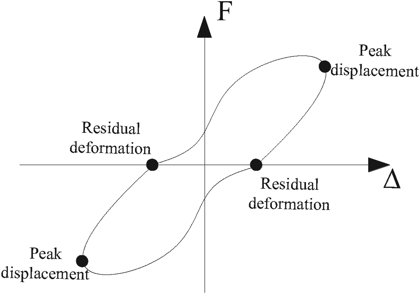

At present, only a few researchers have studied the post-earthquake residual deformation of structures. Kawashima et al. (1998), Ruiz‐ García and Miranda, 2006, Jianbing et al., (2013a, Jianbing et al., 2013b) utilized the elastic-plastic SDOF system to conduct theoretical analysis on the post-earthquake residual displacement of structures. Liepa et al. (2016) proposed a residual displacement vector solution method under the structural vibration theory. Akbari and Khanmohammadi, 2021 comprehensively compared 20 groups of bridge pier numerical models with 6 groups of shaking table tests, and pointed out that the distributed plastic model has strong accuracy in residual displacement prediction. Prior studies have advanced residual-drift evaluation from several angles. For partially self-resetting systems, Bouc–Wen–based restoring-force models with flag-shaped loops have been established, together with simplified estimators of residual drift (Dong et al. 2022, 2024; Feng and Gong, 2020 derived a residual-drift ratio spectrum for main–aftershock sequences via theoretical analysis and dynamics. Zhong et al. (2024) proposed a model for RCCs that links structural period with pulse period, quantifies the vertical-component effect, and enables rapid generation of residual-drift spectra. Collectively, these works provide a solid basis for post-earthquake residual-drift prediction.

For predicting post-earthquake residual deformation of RC members, prior studies span statistical, numerical, and experimental approaches. Zeng et al. (2021) proposed a Bayesian model for RC bridge piers (OpenSees-based) and identified the axial compression ratio as a primary driver of residual displacement. Sun et al. (2016) built an OpenSees model that considers flexure, bond-slip, and shear, and verified its ability to reproduce residual displacement of RC piers. Dong et al. (2023) showed that liquefaction weakens lateral restraint on piles and thus amplifies residual displacement. Wang and Yuhuan, 2024 developed a residual-displacement predictor together with a tri-linear restoring-force model from tests, linking hysteresis characteristics to post-seismic residual deformation. Han et al. (2025) conducted a full-scale test study on composite RCCs, verifying that the steel-FRP hybrid reinforcement system can reduce the residual displacement of column components by about 18.8% while improving ductility and energy dissipation capacity. In addition, Liu et al. (2025) studied the effect of earthquake duration on the residual displacement spectrum of RC bridge piers. Lai and Jiang, 2023 analyzed the residual deformation response of the CRTSII slab track bridge system, established the track-surface mapping relationship, and proposed a calculation method for the residual deformation between bridge deck layers.

Machine learning has increasingly been adopted for residual-drift prediction (Gang and Tong, 2025). Shturmin et al. (2024) developed a residual-drift-angle model for CFT frames and benchmarked six mainstream learners to map drift from geometric and structural inputs. Hu et al. (2022) and Zhang et al. (2023) applied ML at the system scale, improving efficiency and accuracy in seismic-response assessment for steel-braced self-righting hybrids. For bridge applications, Zhou et al. (2022) analyzed an ULRB isolator system with TSD dampers and proposed a probabilistic residual-drift assessment based on a tri-segment hysteresis formulation. Liu et al. (2022) used an operator-splitting (ALE) approach to simulate caisson wharves under liquefaction and found that residual settlement scales nearly linearly with peak seismic load, while pore-pressure connection zones amplify drift. In addition, Zheng et al. (2023) reviewed the application potential of artificial intelligence in seismic assessment and pointed out that data-driven AI methods have significant advantages in ground motion identification, rapid post-earthquake assessment, and residual displacement prediction.

RCCs are important seismic components of building structures. The degree of damage after an earthquake directly affects the overall safety and functional recovery capacity of the structure. To this end, scholars have proposed a variety of methods for post-earthquake damage assessment of RCCs, which can be grouped into three categories: damage index method based on empirical models, assessment method based on response characteristics, and classification prediction method based on intelligent algorithms. The most classic damage assessment method includes Park- Ang damage index (Park et al., 1985), which measures the degree of component damage by hysteresis energy dissipation and maximum deformation. Although it has certain physical significance, the model parameters rely on experimental calibration and have poor versatility. In recent years, in order to further improve the quantification and applicability of the assessment, researchers have begun to focus on residual deformation as a key criterion. For example, Zhao et al. (2021) proposed a RC bridge pier damage assessment model based on residual displacement, which comprehensively considers the influence of environmental corrosion factors and axial compression ratio on damage evolution. In addition, Shan et al. (2021) constructed an intelligent assessment framework that combines feature classification and model optimization, which can effectively improve the accuracy and efficiency of damage identification. In terms of non-contact assessment, image recognition and structural response signal processing technology are gradually introduced into the post-earthquake assessment of RC components. Combined with methods such as neural network (CNN) and support vector machine (SVM), automatic identification and classification of component cracks, deformation and damage distribution are attained (Azhari et al., 2025; Jamshidian and Hamidia, 2023). This direction demonstrates strong application prospects in the construction of post-earthquake rapid assessment systems. Although RCCs may not be completely destroyed after an earthquake, their strength, stiffness and ductility are generally severely weakened (Gang et al., 2023). Therefore, evaluating their residual bearing capacity is of great value in deciding whether to repair, reinforce or demolish them. Existing research is mainly carried out through three paths: experimental testing, finite element analysis and data-driven prediction methods. In terms of experimental research, Li et al. (2023) analyzed the RSC of RCCs under different earthquake damage levels based on the damage distribution model and proposed a functional relationship between the damage index and the residual bearing capacity. Li et al. (2020) utilized the PEER database to construct a numerical model and systematically analyzed the coupling effects of key design parameters of components, earthquake damage degree and residual bearing capacity. In addition to experiments and modelling, intelligent prediction methods have also become a research hotspot in recent years. By integrating pre-earthquake design information, earthquake input parameters and post-earthquake damage indicators, researchers have constructed a variety of machine learning models such as SVR, random forest (RF) and deep neural network (DNN), which significantly improved the accuracy and computational efficiency of residual bearing capacity prediction. For example, the classification-regression integrated model proposed by Shan et al. (2021), that is, classifying the damage state by feature clustering, and then introducing a prediction sub-model to estimate the bearing capacity, demonstrates strong engineering adaptability. In addition, Japan and other places have introduced the RSC index R (RSC Index) at the practical level for rapid screening of the repair and use level of buildings after an earthquake. Maeda and Kang (2009) proposed a calculation method and engineering criteria for it, laying the foundation for the standardization of the post-earthquake assessment system. Data-driven time-series modeling is increasingly used to predict deformation and assess the seismic performance of RC structures under various earthquakes. Zhang et al. (2024) proposed a post-earthquake damage-state evaluation framework and validated it experimentally, linking response indicators to practically interpretable damage states. Shan et al. (2024) combined spatiotemporal clustering, empirical mode decomposition, and LSTM to improve multi-step deformation prediction for complex monitoring data. While these advances confirm the strength of LSTM-type models for time-dependent response prediction, further work is needed to translate predicted deformation histories into hysteresis reconstruction and damage-related metrics for engineering assessment.

Most prior studies on RCC residual drift focus on prediction and rarely treat it as an explicit index for post-earthquake performance. Evidence shows this measurable metric correlates with observed damage and remaining capacity, enabling quantitative post-event assessment. Residual drift is governed by loading history, material strengths, member size, and stress state, yet conventional formulations struggle to capture these coupled effects. Recent machine-learning advances offer practical means to model the nonlinear, multivariate relation between inputs and column response under earthquakes.

Utilizing experimental data from hysteresis curves that capture the full-range behavior of RCCs (from elastic response to damage phases), multiple optimized ML models are developed to predict the peak seismic deformation, deformation capacity, and complete hysteresis response based on residual displacements and key column parameters. Building on these predictive models, we develop a quantitative model to assess post-earthquake damage and RSC. These models realize fast, data-driven damage and residual capacity assessment, overcoming the limitations of traditional methods. This study aims to provide a reliable tool to evaluate the post-earthquake RSC of RCCs and support decision-making for structural rehabilitation, strengthening, and resilience planning.

This study advances post-earthquake assessment of RCCs by introducing an integrated, data-driven framework that converts a measurable indicator—residual drift—into both damage curves and RSC.

Framework. To the best of our knowledge, we propose the first end-to-end evaluation framework that integrates three ML models—ML-Pd (peak deformation), ML-Dc (deformation capacity), and ML-Hc (full hysteresis)—to jointly quantify post-earthquake damage and residual seismic capacity (RSC) from residual drift.

Database and protocol. Compile and use a 326-specimen RC-column database with a clear 80/20 train–test split and minimal, leakage-free preprocessing (imputation, duplicate removal, normalization).

Models and interpretability. Employ optimized tree-boosting (XGBoost/GB) for ML-Pd/ML-Dc and a fixed LSTM(n32) for ML-Hc to capture path dependence, pinching, and degradation.

Validation and results. Demonstrate high accuracy on a held-out test set (ML-Pd/ML-Dc: R² ≥ 0.94; ML-Hc: R² ≈ 0.99), visualize 10 test-set exemplars for damage curves, quantify residual capacity across residual-drift levels, and provide five full-scale tests for external verification.

Practical deliverables. Output damage–residual-drift curves and RSC that can be directly used in rapid screening, repair/retrofit decisions, and resilience planning.

Methods

Research motivation

Based on the cyclic loading tests of RCCs in the past, the seismic damage evolution of RCCs can be described from no earthquake - small earthquake - moderate earthquake - large earthquake – destruction as shown in Figure 2. Then, where “Loading cases” is the cyclic loading history of RCCs converted from different earthquake intensities, “Column surface damage and residual displacement” represent the surface cracks and concrete damage and residual displacement of RCCs, “seismic response” represents the response of RCCs under different earthquake intensities, and “post-seismic residual seismic capacity (RSC)” represents the hysteresis curves of the earthquake-damaged columns from reloading to failure. The post-earthquake RSC of an RCC refers to its ability to continue to serve after experiencing earthquake damage. It can be found that.

(1) When there is no earthquake, that is, when the RCC is in normal service, there are no cracks on the surface and no residual displacement (dr) is generated. It is observed that the RSC of the RCC is its full-range hysteresis curves.

(2) As the earthquake intensity increases, cracks begin to appear on the surface of the RCC. At this stage, the nonlinear characteristics of the hysteresis curves become stronger, the envelope area of the hysteresis loop becomes larger (as shown in the “Seismic response” in Figure 1), and the residual displacement of the RC becomes larger (as shown in the “Column surface damage and residual displacement” in Figure 1). At this time, it can be found that when the RCC is reloaded after the earthquake, its hysteresis curve loses its elastic section. When the displacement is 0, its load is not at point 0, thereby leading to residual displacement (d_r).

(3) When the RCC is loaded to a certain extent, concrete crushing occurs. As the crushing area increases, a yield section will appear in the seismic response hysteresis curves. At this time, the residual displacement of the RCC increases rapidly. After the earthquake, the deformation of the RCC will remain at the residual displacement. When loaded again, its stiffness will decrease and appear in a pinched state, as shown in the hysteresis curves characterized by RSC.

(4) When the RCC is loaded to failure, a large area of concrete is crushed on its surface. At this time, the residual displacement of the RCC reaches its maximum value, and the seismic response is a hysteresis curve of the entire process of elasticity-plasticity-failure of the RCC. At this time, the RCC cannot be reloaded, and its RSC is 0.

Figure 2.

Damage evolution and residual deformation mapping of RCCs under increasing seismic intensity.

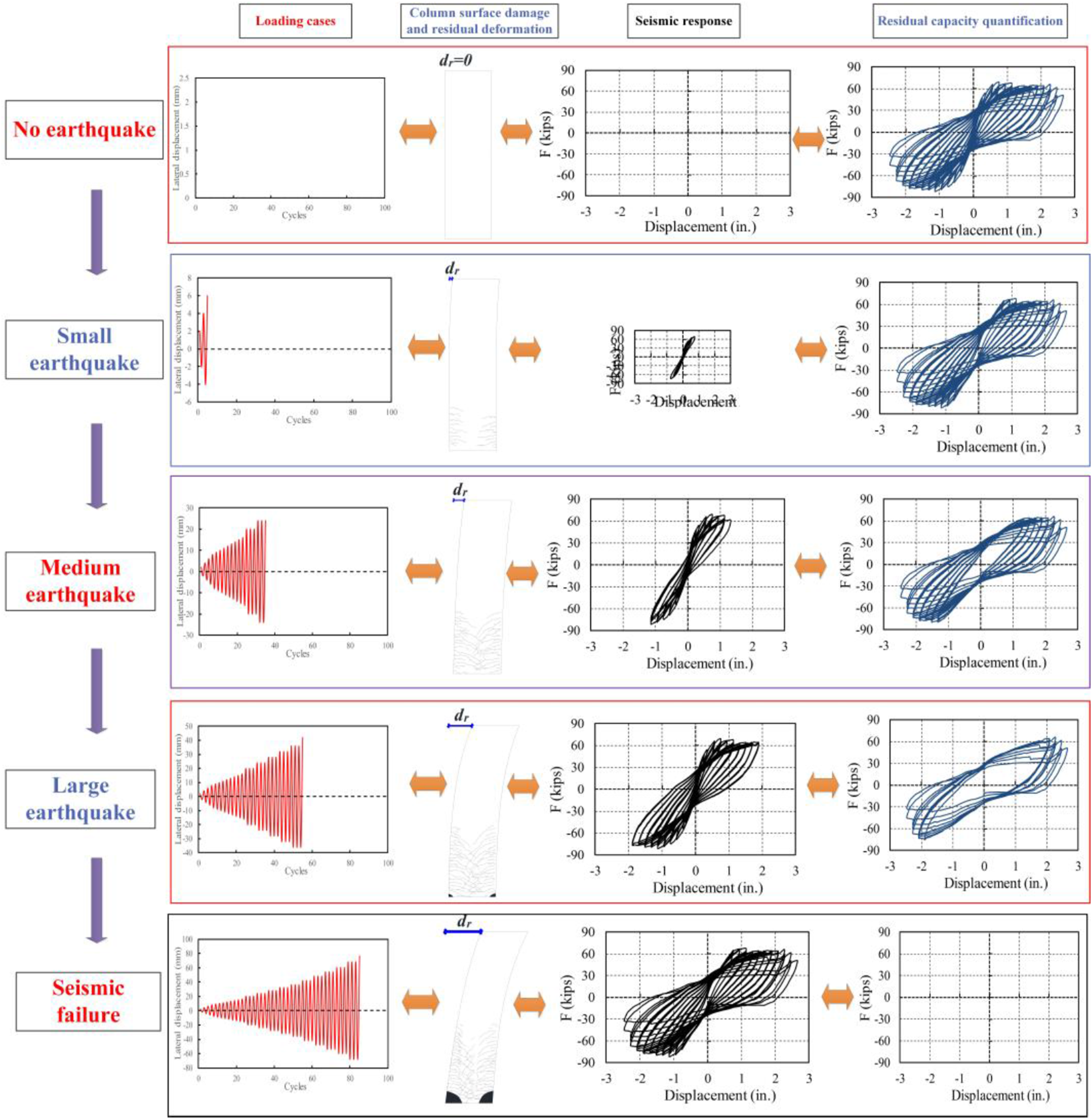
Surface cracking and concrete distress correlate strongly with the residual displacement of RCCs. Unlike visual damage measures, residual displacement is directly measurable and reproducible. We therefore adopt residual displacement as the core evaluation index for post-earthquake assessment, enabling an objective and quantitative estimate of RCC damage and RSC.

Overview of proposed framework

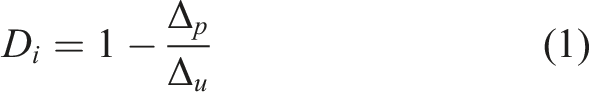
In the study of the seismic performance of RCCs, cyclic loading tests are usually utilized to obtain the displacement-load hysteresis curves of the entire process from elasticity to plasticity to destruction. This curve records the loading-deformation behavior of RCCs during small, medium, and large earthquakes and even during destruction, so that the performance state of RCCs can be comprehensively quantified, including key parameters such as deformation capacity, energy dissipation characteristics, and residual displacement. In previous performance evaluations, many scholars utilized the peak deformation of the structure in an earthquake as the performance index of the RCC (Li and Zhang, 2021; Mahin and Moehle, 2024). This index can more clearly reflect the earthquake intensity and the degradation degree of the structural performance after the earthquake. Therefore, in order to effectively quantify the damage degree of the RCC, this study defines the seismic damage index of the RCC as shown in equation (1), that is:

D_{i} = 1 - \frac{Δ_{p}}{Δ_{u}}

(1)

Where: Δp and Δu are respectively peak and ultimate deformation of the RCC caused by an earthquake. It is observed that when the lateral deformation is small, the larger Di is, indicating that the damage to the RCC is smaller. This damage index is reasonable and intuitive, and its physical meaning is clear. However, in general, most structures are not equipped with sensors, and the peak deformation of the structure caused by an earthquake cannot be obtained. Existing finite element analysis is difficult to fully consider factors such as material damage, concrete cracks and crushing, thereby leading to inaccurate residual capacity predictions.

The RSC of RCCs is affected by multiple parameters and has strong nonlinear characteristics. Traditional post-earthquake assessments rely on qualitative observations of surface cracks and concrete crushing, making it difficult to quantify the damage degree and the RSC. And it is also impossible to predict the bearing, deformation, energy dissipation capacity and stiffness degradation in subsequent earthquakes. ML technology provides an effective way to solve this problem.

To this end, this study proposes a method for evaluating the post-seismic performance and predicting the RSC of RCCs based on ML, as shown in Figure 3.

(1) Database construction: The full-range hysteresis curve test data of RCCs are collected, and the residual displacement data under different loading conditions are extracted. The data are combined with the structural parameters of the RCCs, such as size, reinforcement, and axial compression, to form a database for training the machine learning model.

(2) Peak deformation prediction under different seismic conditions (ML-Pd): Using different ML methods (such as XGBoost and CatBoost), combined with residual deformation and structural parameters, a peak deformation prediction model (ML-Pd) of RCCs under different seismic cases is established.

(3) Prediction of deformation capacity of RCC under cyclic loading (ML-Dc): Based on the full-process hysteresis curve test data of RCCs, the deformation capacity test data of each specimen were extracted. Combined with the structural parameters, a deformation capacity prediction model (ML-Dc) was established using ML methods.

(4) Full-range hysteresis curve prediction (ML-Hc): Using multivariate time series deep learning models (such as LSTM, BiLSTM), combined with the size, reinforcement, axial load (ratio) and other information of RCCs, a full-range displacement-load hysteresis curve prediction model (ML-Hc) including elasticity-plasticity-destruction statues of RCCs is established.

(5) Calculation of seismic damage index: Based on the ML-Pd and ML-Dc models and combined with the seismic damage index formula (Equation (1)), the damage index under different residual displacements is calculated to generate the full-range seismic damage curve of the RCC.

(6) RSC assessment: Given a measured post-earthquake residual displacement of an RCC, ML-Pd estimates the peak deformation that was reached. Combined with ML-Hc, which predicts the hysteresis from that peak through continued loading to failure, the loading history is reconstructed and the RSC is obtained.

Figure 3.

Proposed ML-based framework for post-earthquake damage assessment and RSC prediction of RCCs.

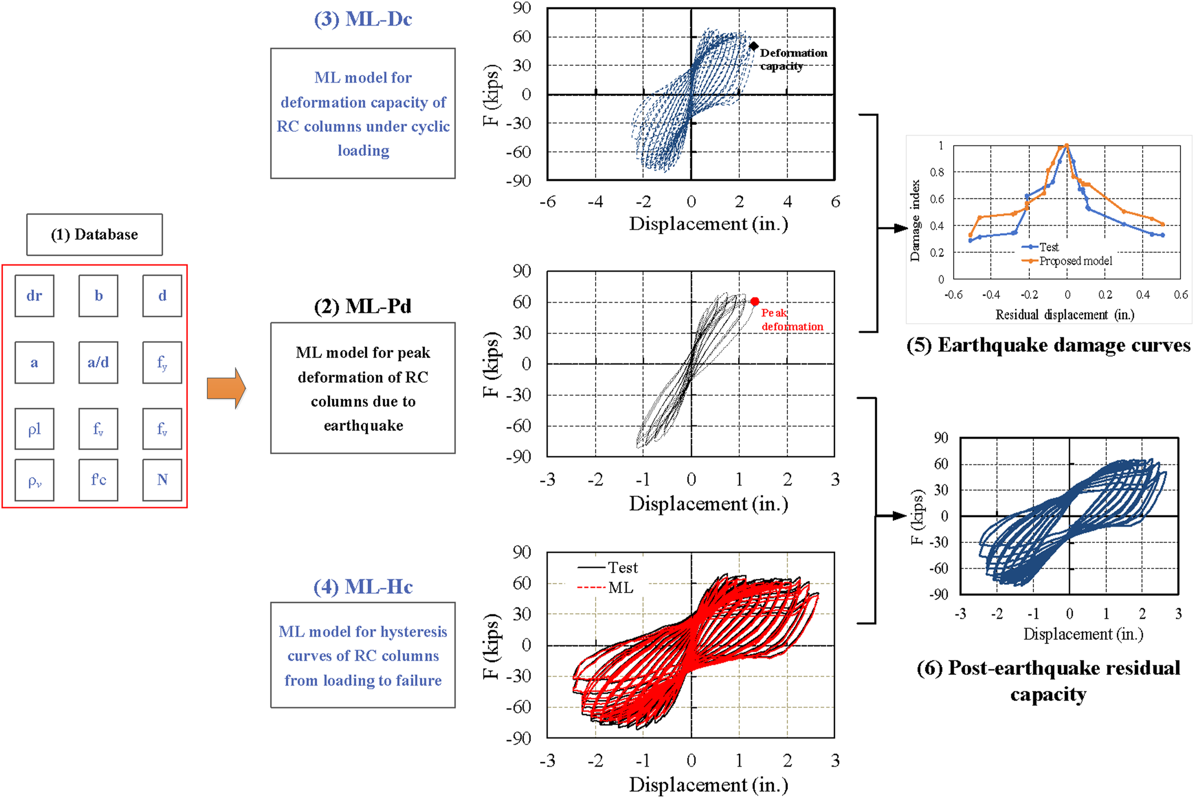
This data-driven procedure enables quantitative, rapid post-event evaluation, addresses limits of conventional judgment-based methods, and provides practical support for repair and strengthening decisions.

Database establishment

Load-displacement hysteresis records for 326 RC columns were sourced from the NEES–ACI 369 database (Ghannoum et al., 2015). The source provides 27 descriptors; after screening for mechanical relevance and completeness, 16 variables were retained. Residual displacement dr is defined as the zero-force displacement at the end of a cycle (Figure 1) and is used as a key predictor/response in the models. Figure 4 schematically define the section dimensions and the loading configurations; units follow the original database (in, in², psi, kips). The retained inputs cover: geometry (b, h, d, a, a/d); longitudinal reinforcement (As1, Asm, As2, ρL, fy); transverse reinforcement (ρv, fv); concrete strength (fc′); axial demand (N, n); and the test configuration (single-cantilever, double-cantilever, or double-curvature, encoded as 1/2/3) (Figure 5).

Figure 4.

Cross-sectional schematic of a typical RCC specimen.

Figure 5.

Test configurations of RCCs.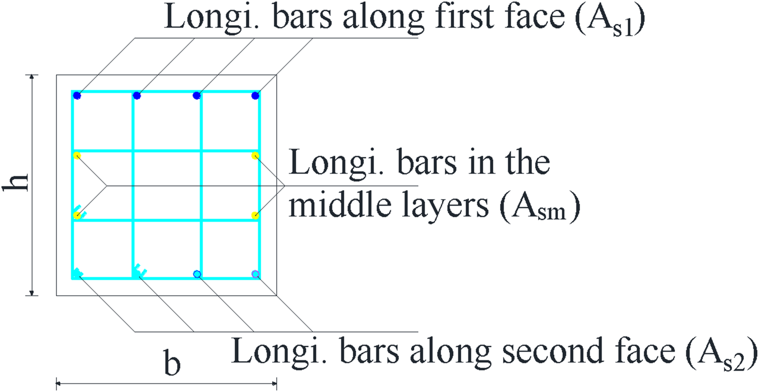

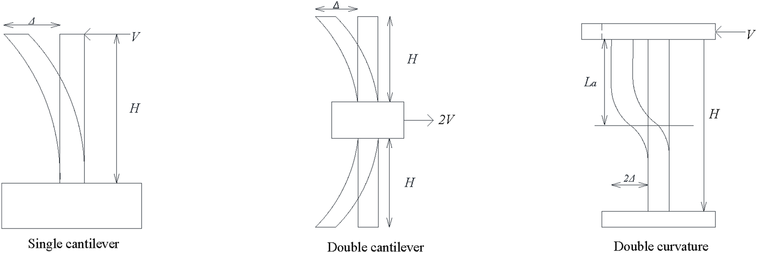
Figure 6 shows the distributions of all inputs, and Figure 7 reports their descriptive statistics. Section dimensions exhibit wide dispersion: h = 12.5 ± 4.7 in, b = 11.8 ± 4.9 in, and effective depth d = 10.9 ± 4.4 in; the shear span has the largest spread, a = 41.5 ± 22.5 in. The longitudinal steel areas A_s1, A_s2, A_sm have similar means, indicating balanced reinforcement layouts across specimens. Steel yield strength is relatively uniform (f_y = 62,040 ± 8,908 psi), whereas concrete strength spans a broad range (f_c′ = 1,900∼17,110 psi). Axial load N is highly dispersed (233.9 ± 280.3233.9 kips), while the axial ratio n is more moderate (0.24 ± 0.18). The quartiles in Figure 6 are consistent with these patterns, confirming substantial heterogeneity in the experimental program.

Figure 6.

Distribution of key structural and material parameters in the experimental dataset.

Figure 7.

Dataset statistics.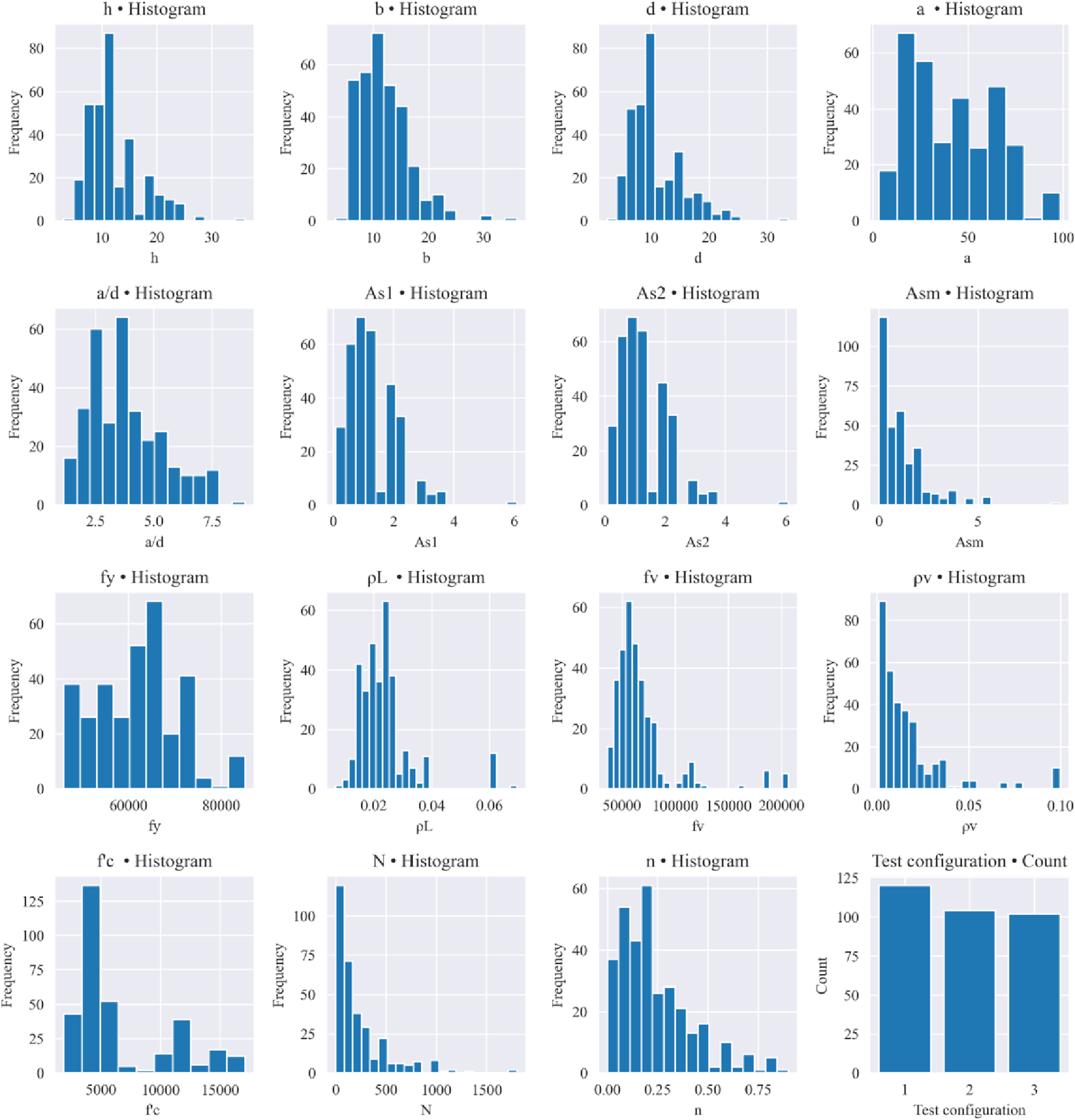

Our preprocessing deliberately remained simple and transparent: (i) we performed missing-value checks and imputed missing numeric entries with the median and categorical entries with the mode; (ii) we removed duplicates based on specimen/program identifiers; and (iii) we applied feature normalization (min–max scaling to [0, 1]) to the predictors. All imputers and scalers were fit on the training portion only and then applied to validation/test folds to prevent leakage. Specimens without the core variables required for the target tasks were excluded; no additional smoothing or outlier filtering was applied so as not to alter measured responses.

Machine learning model building

ML- Pd and ML-Dc

We built two predictors—ML-Pd for peak deformation and ML-Dc for deformation capacity under cyclic loading—and benchmarked eight regressors: SVR, Decision Tree, Random Forest, Gradient Boosting, MLP, XGBoost, LightGBM, and CatBoost. During model development, we used five-fold cross-validation and ensured that all preprocessing operators (imputers/scalers) were fit exclusively on the training folds before being applied to the held-out fold. Hyperparameters were tuned within the training portion only, and all metrics are reported on the corresponding held-out folds. This preserves a clean separation between training and evaluation while remaining faithful to the simple preprocessing pipeline described above. Performance was evaluated using R², MSE, RMSE, and MAE. All models used the same train–test split (and identical preprocessing) to ensure a fair comparison.

ML-Hc

Challenges and solutions

As shown in Figure 8, low-cycle loading produces a strongly nonlinear evolution of the hysteresis response. Three features are prominent: pinching, strength/stiffness degradation, and path dependence. In Figure 8(a)), at the same displacement Δ1 the forces on the loading and unloading paths (F1 and F2) differ, so the F–Δ relation is multi-valued and history-dependent. With continued cycling, the envelope shrinks and the loop shape changes (Figure 7(b)), confirming strong memory of prior loading. Models that rely on single-valued constitutive relations or static regressions—i.e., treating the current response as a function of the current input only—cannot reproduce the “same Δ, different F” behavior or the causal evolution of degradation, often resorting to ad-hoc coefficients with limited generality.

Figure 8.

Characteristics of hysteresis behavior in RCCs: (a) Difference in loading and unloading paths at same displacement; (b) Degradation and shrinkage of hysteresis loops over repeated cycles.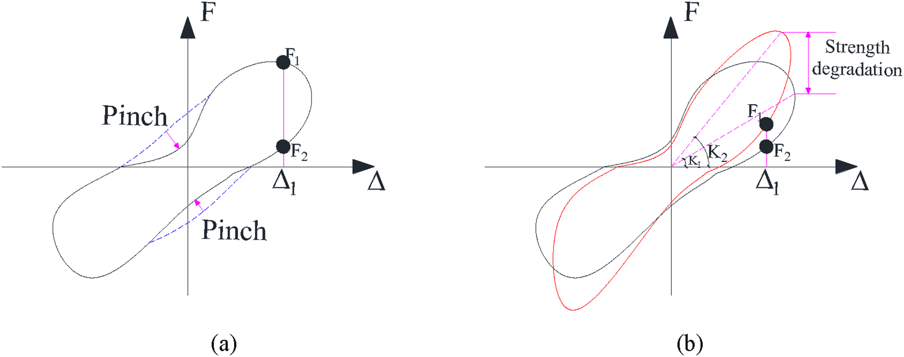

Multivariate time-series neural networks are well suited to hysteresis modeling for three reasons. First, gated memory (e.g., LSTM) encodes loading history, allowing the model to distinguish loading and unloading branches at the same displacement and to recover the path-dependent gap in the F–Δ loops. Second, they accept multiple predictors—axial compression ratio, shear-span ratio, material strengths, and reinforcement ratios—so cross-variable interactions are learned rather than prescribed. Third, by treating the hysteresis as a dynamic sequence, they generate the response step-by-step and track envelope shrinkage, pinching, and stiffness/strength degradation across cycles. This reduces reliance on ad-hoc coefficients and improves robustness across different loading protocols.

From the above diagrams and theoretical analysis, the hysteresis response modelling of RCCs has complex characteristics such as strong nonlinearity, multivariable coupling, degradation evolution, and time path dependence. The use of multivariate time-series deep neural networks not only conforms to the physical mechanism, but also provides an effective technical path for achieving full-range, high-precision hysteresis curve prediction.

Establishment of multivariate time series model

An LSTM augments a recurrent unit with three gates—forget, input, and output, shown in Figure 9—that regulate how much past information is carried forward and how much new information is written to the cell state (Greff et al., 2017). This gating lets the network retain loading history over long spans and distinguish loading vs. unloading branches at the same displacement. Model capacity is controlled by the number of hidden units; in our experiments we use a single-direction LSTM to roll the response forward from the identified peak.

Figure 9.

LSTM memory cell with forget, input, and output gates controlling updates to the cell state.

A BiLSTM stacks two LSTMs that read the sequence in opposite directions and then concatenates their outputs (Graves and Schmidhuber, 2005), shown in Figure 10. The architecture provides richer context when the entire record is available (e.g., offline fitting or diagnostics). In this study, it serves as a reference model; the forward LSTM remains the main predictor for step-ahead hysteresis generation.

Figure 10.

Bidirectional LSTM: forward and backward LSTMs process the same sequence and their outputs are concatenated.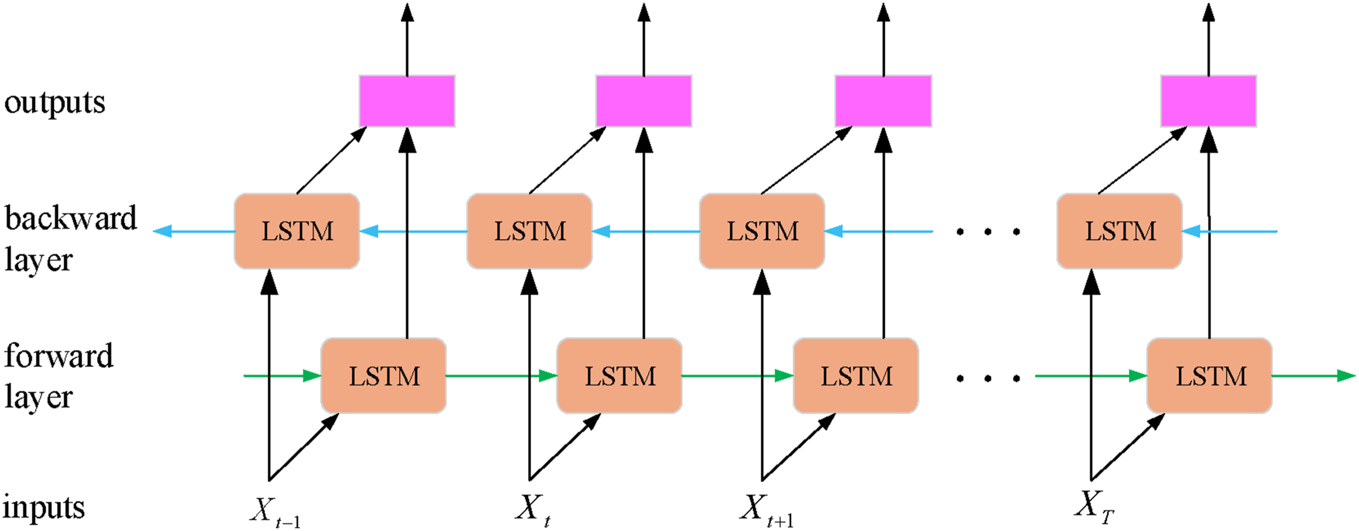

We model hysteresis as a multivariate time-series problem and train LSTM and BiLSTM variants (Figures 9 and 10). LSTM’s gated memory captures path dependence and pinching; the width n controls capacity. We test n = 4/8/16/32. BiLSTM (32 units) is included as an ablation to assess context aggregation.

Evaluating the predictive performance of ML models

We use a specimen-level 80/20 split (261/65). ML-Pd and ML-Dc are tuned by grouped 5-fold CV on the 261-specimen pool; all test metrics use the same 65-specimen hold-out set. ML-Hc uses a fixed LSTM(n = 32) chosen from a small width ablation (n = 4/8/16/32; BiLSTM (n = 32)); no hyperparameter search was run due to compute constraints.

ML-Pd model

ML-Pd model is utilized to predict the peak deformation of RCC specimens under different residual displacements. Figure 11 demonstrates the prediction-actual comparison scatter plot of each ML model on the training and test sets, and Table 1 summarizes the performance indicators.

Figure 11.

Predicted vs. measured peak deformation of RCCs under various residual displacements.

Table 1.

Prediction model of peak deformation of RCCs under different residual displacements.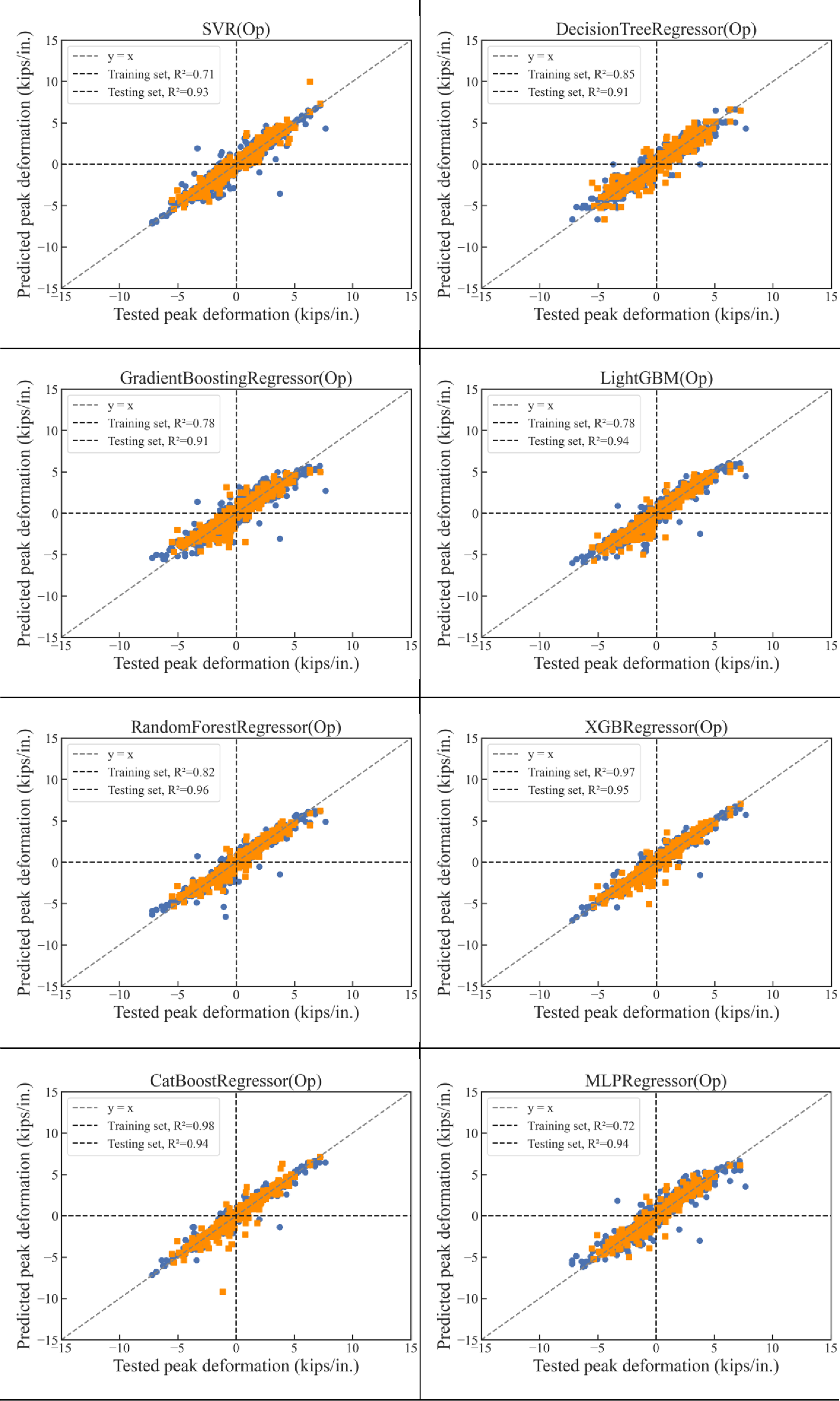

Model	Train				Test
Model	MSE	MAE	RMSE	R²	MSE	MAE	RMSE	R²
SVR (Op)	0.95	0.26	0.98	0.71	0.16	0.27	0.40	0.93
DT (Op)	0.20	0.26	0.44	0.85	0.20	0.25	0.44	0.91
GB (Op)	0.71	0.28	0.84	0.78	0.20	0.27	0.44	0.91
CatBoost (Op)	0.05	0.13	0.23	0.98	0.15	0.19	0.38	0.94
RF (Op)	0.57	0.13	0.75	0.82	0.09	0.17	0.30	0.96
XGBoost (Op)	0.09	0.16	0.29	0.97	0.12	0.19	0.34	0.94
LightGBM (Op)	0.70	0.19	0.84	0.78	0.13	0.20	0.37	0.94
MLP (Op)	0.91	0.23	0.95	0.71	0.14	0.22	0.37	0.94

The R² values of CatBoost, XGBoost, Random Forest and MLP models on the test set all exceed 0.94, showing extremely high prediction accuracy. Among them, CatBoost attained the lowest error on the training set (MSE = 0.05, RMSE = 0.23, R² = 0.98), and also performed well on the test set (R² = 0.94), indicating its strong generalization ability for the peak deformation under different residual displacements. The ensemble learning models such as Gradient Boosting, XGBoost, LightGBM and CatBoost all show a strong point group distribution in the figure, and the predicted values deviate less from the true values, and the residual distribution is relatively uniform. Among them, the XGBoost prediction value is closest to the ideal line y = x, and has a high R² value (0.97 and 0.94) on both the training and test sets, showing high stability and accuracy. Although decision trees (DT) and SVR can capture certain regularities, their R² values on the training set or test set are 0.85/0.91 (DT) and 0.71/0.93 (SVR), respectively, which means they have a certain degree of underfitting or overfitting risk. In addition, the error of SVR on the training set is relatively large (MSE = 0.95, RMSE = 0.98), while it has a higher R² value on the test set, indicating that it may be too dependent on the data feature boundary and underfit the training data. The MLP model has an R² of 0.94 on the test set and a medium level of error (MSE = 0.14, RMSE = 0.37), showing its strong nonlinear feature extraction ability.

We evaluated eight representative tabular regressors under identical data splits and five-fold cross-validation. XGBoost (Op) was selected for ML-Pd because it consistently delivered the most stable generalization while capturing key nonlinear interactions among axial load ratio, reinforcement ratios, and material strengths. Simpler trees or SVR showed under/over-fitting on our data, whereas CatBoost/LightGBM were competitive but did not yield a consistent gain over XGBoost. Beyond accuracy, XGBoost is advantageous for interpretability and practical use (fast inference, robust handling of heterogeneous tabular inputs, modest memory footprint, and mature deployment tooling). These properties make it suitable for engineering workflows where explanations, quick what-if checks, and portability are required.

For reproducibility, the tuned settings of XGBoost (Op) are: learning_rate = 0.10, max_depth = 3, n_estimators = 50, subsample = 1.0. Other parameters follow the library defaults. Preprocessing (missing-value imputation and min–max normalization) was fit on the training portion only; these values were fixed for all test evaluations.

ML-Dc model

XGBoost algorithm was utilized to establish a deformation capacity prediction model for RCCs under cyclic loading, and the prediction ability of the model was evaluated. The various prediction accuracy evaluation indicators are shown in Table 2, and the predicted and experimental results of the deformation capacity is shown in Figure 12. Under the identical split and five-fold CV, the XGBoost family provided the satisfied generalization for deformation-capacity prediction. Compared with the base model, the hyperparameter-optimized variant XGBoost (Op) improved test goodness-of-fit and squared-error metrics (R²: 0.93 → 0.94; MSE/RMSE: 0.24/0.42 → 0.16/0.40) while keeping strong train performance (R² 0.96; MSE 0.11; MAE 0.23). The test MAE increased from 0.18 to 0.25, indicating a higher average absolute error but fewer large errors, which is desirable for safety-critical capacity estimation where outliers are penalized quadratically (by MSE/RMSE) and under-prediction must be tightly controlled. Accordingly, we report XGBoost (Op) as the default Dc predictor, and retain the base XGBoost as an ablation highlighting lower MAE. In practice, the XGBoost family also offers clear interpretability and operational practicality (fast inference, modest memory, mature tooling), facilitating auditability and “what-if” checks in engineering workflows.

Table 2.

Deformation capacity prediction model of RCCs.

Model	Train				Test
Model	MAE	MSE	RMSE	R²	MAE	MSE	RMSE	R²
XGBoost	0.23	0.12	0.34	0.95	0.18	0.24	0.42	0.93
XGBoost (Op)	0.23	0.11	0.33	0.96	0.25	0.16	0.4	0.94

Figure 12.

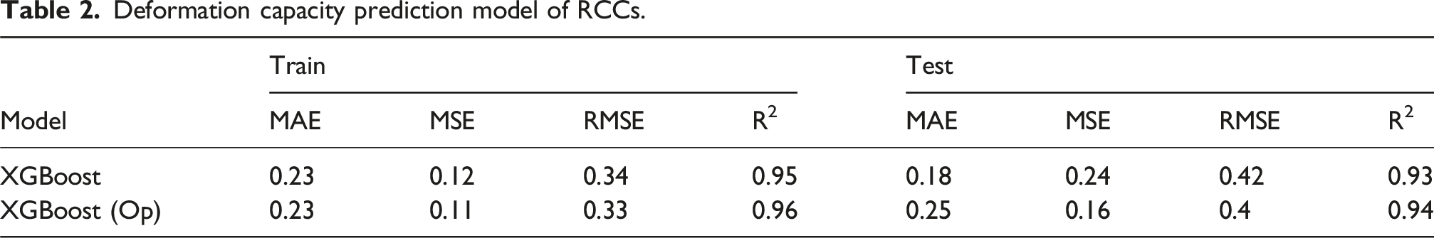
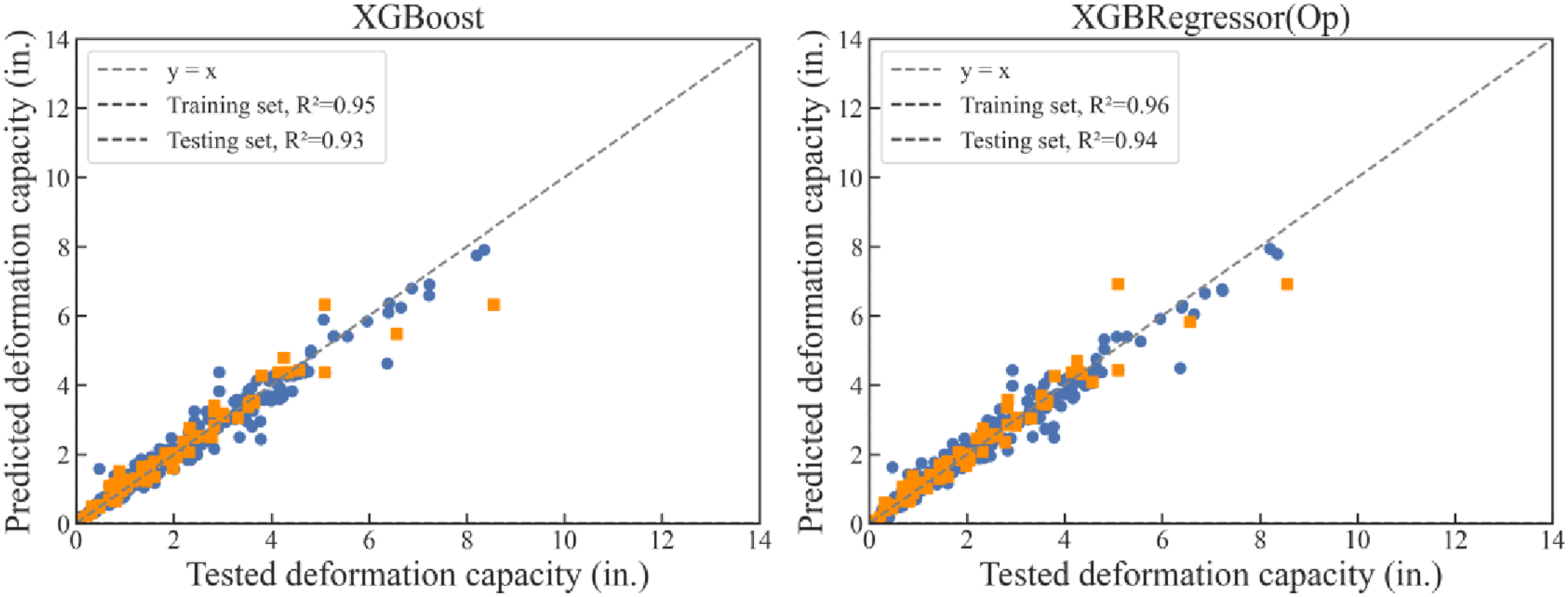
Comparison of predicted and measured deformation capacity.

Final hyperparameters (ML-Dc; XGBoost (Op)). The optimized settings are: learning_rate (0.10), max_depth (3), n_estimators (200), subsample (0.8). Other parameters use defaults. Compared with ML-Pd, the larger number of trees and partial subsampling improved stability near capacity limits; preprocessing was identical and fit on the training portion only.

ML-Hc model

We use a single-direction LSTM with different hidden units (activation = relu), followed by Dropout (0.2) and a Dense (1) output. Training adopts MSE loss and Adam, up to 100 epochs with early stopping (monitor = val_loss, patience = 10), using validation_split = 0.1, batch_size = 64, and shuffle = False. The model is trained once on the 80% training portion and evaluated on the same fixed 20% hold-out set; no hyperparameter search is performed.

Figure 13 summarizes the prediction ability of the models on the RCC specimens of test set. The hysteresis-trajectory task is inherently time-dependent with path memory, pinching, and strength/stiffness degradation. LSTM directly addresses these properties through gated memory, enabling learning of causal load–unload–reload effects. Increasing hidden units improves accuracy: LSTM(n4) yields MAE 8.83 and R² 0.73, whereas LSTM(n32) reaches MAE 1.53 and R² 0.99 on the test set. LSTM(n16) (MAE 2.11, R² 0.99) sits between these settings. LSTM(n32) achieved the lowest error among the RNN variants at the same R² (MAE 1.53; MSE 4.45; R² 0.99), slightly outperforming BiLSTM(n32), while requiring fewer parameters and avoiding bidirectional look-ahead (thus aligning with physical causality and reducing latency). These results support selecting LSTM(n32) for ML-Hc on both accuracy and practicality grounds.

Figure 13.

Performance evaluation of each model prediction test set.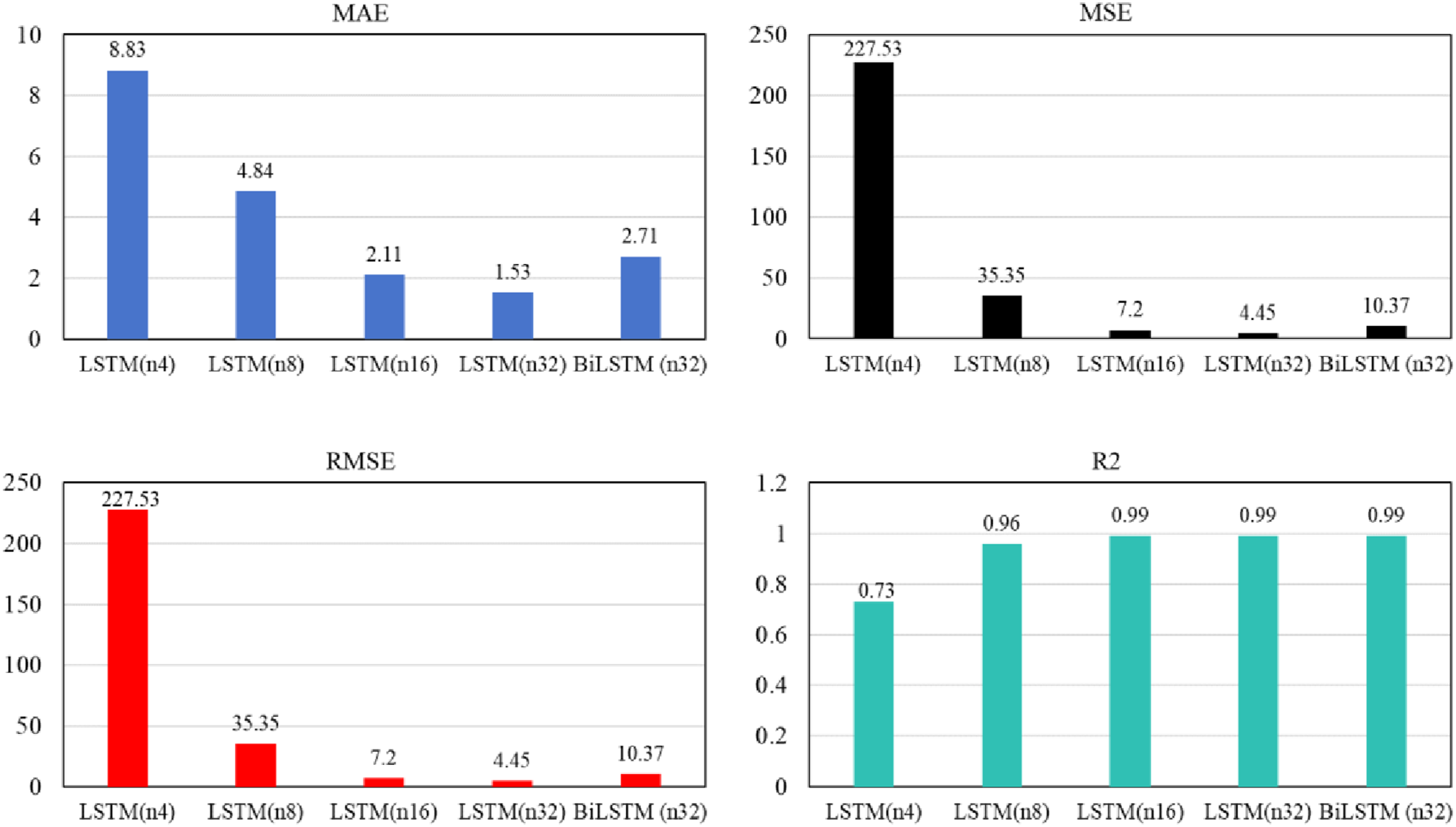

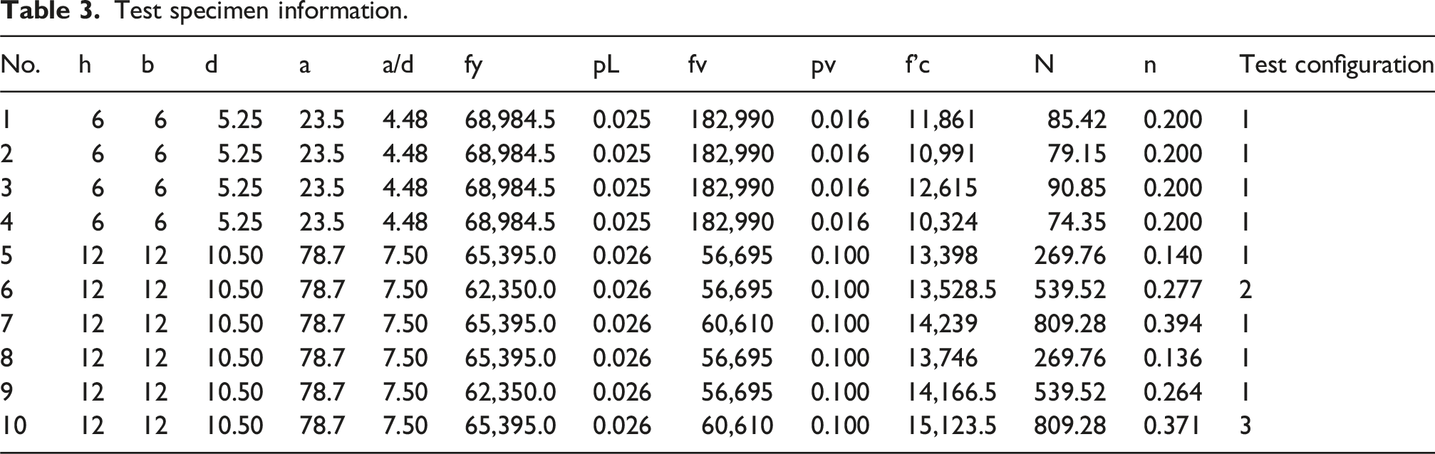
We assess the hysteresis predictor on key aspects—strength, stiffness, pinching/degeneration, and energy dissipation. Ten RC columns were randomly selected from the fixed 65-specimen hold-out set (Table 3). For each specimen, the trained ML-Hc generated the hysteresis loops, which were overlaid with the corresponding test records. Figure 14 shows the comparisons: red dashed curves are ML predictions and black solid curves are experiments.

Table 3.

Test specimen information.

No.	h	b	d	a	a/d	fy	pL	fv	pv	f'c	N	n	Test configuration
1	6	6	5.25	23.5	4.48	68,984.5	0.025	182,990	0.016	11,861	85.42	0.200	1
2	6	6	5.25	23.5	4.48	68,984.5	0.025	182,990	0.016	10,991	79.15	0.200	1
3	6	6	5.25	23.5	4.48	68,984.5	0.025	182,990	0.016	12,615	90.85	0.200	1
4	6	6	5.25	23.5	4.48	68,984.5	0.025	182,990	0.016	10,324	74.35	0.200	1
5	12	12	10.50	78.7	7.50	65,395.0	0.026	56,695	0.100	13,398	269.76	0.140	1
6	12	12	10.50	78.7	7.50	62,350.0	0.026	56,695	0.100	13,528.5	539.52	0.277	2
7	12	12	10.50	78.7	7.50	65,395.0	0.026	60,610	0.100	14,239	809.28	0.394	1
8	12	12	10.50	78.7	7.50	65,395.0	0.026	56,695	0.100	13,746	269.76	0.136	1
9	12	12	10.50	78.7	7.50	62,350.0	0.026	56,695	0.100	14,166.5	539.52	0.264	1
10	12	12	10.50	78.7	7.50	65,395.0	0.026	60,610	0.100	15,123.5	809.28	0.371	3

Figure 14.

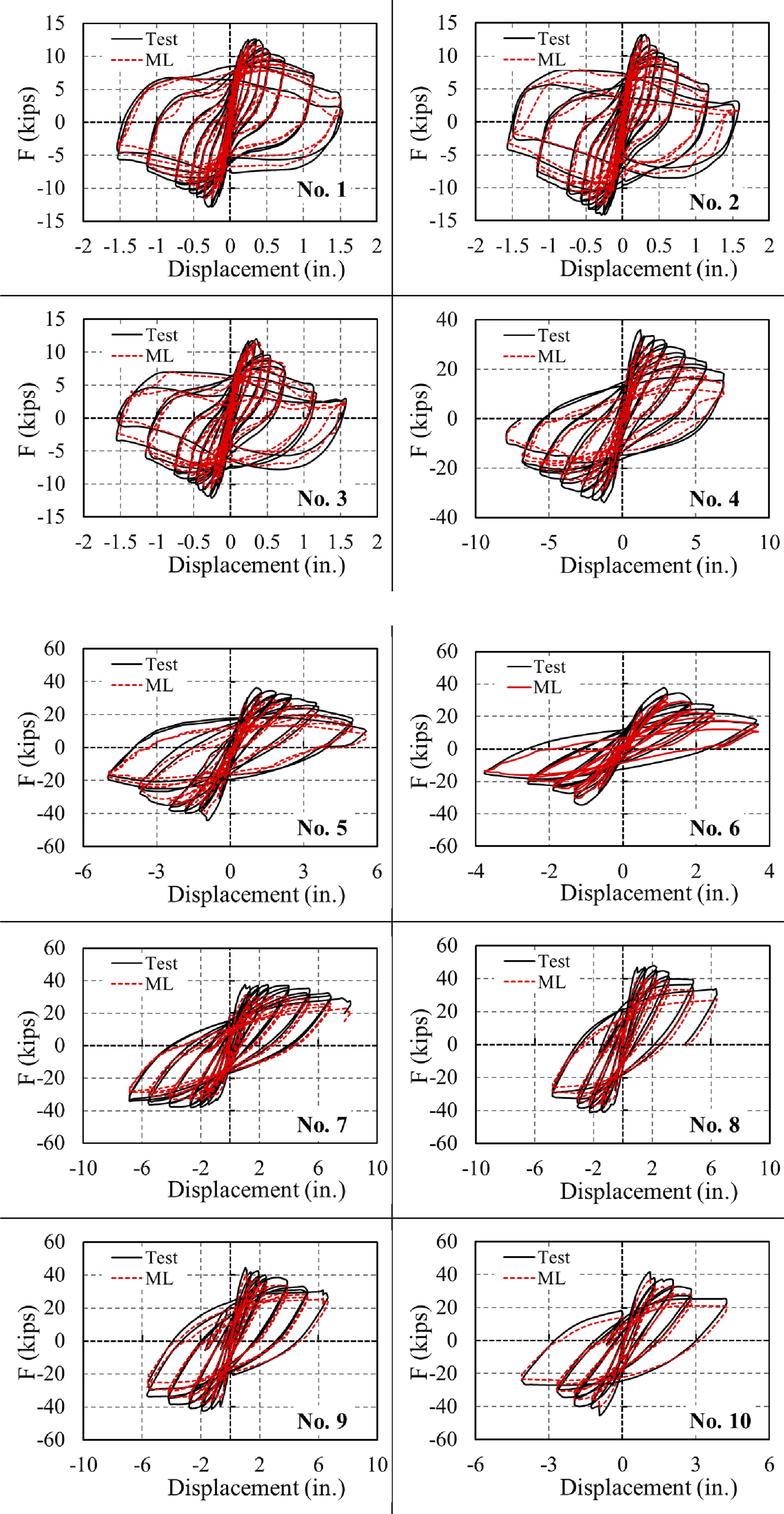
Predicted vs. measured full-range hysteresis loops for selected RCCs from the hold-out test set (red dashed: ML-Hc prediction; black solid: experiment).

Overall, the model reproduces experimental hysteresis with high fidelity. Across the test columns, the predicted loops match the measured envelope and symmetry, capturing peak strength, stiffness/strength degradation, and pinching. Main-loop areas and turning points align with tests, indicating that deformation-path effects are learned rather than pointwise fitted. The maximum lateral capacity is estimated accurately, with the predicted backbone generally coinciding with the experimental envelope. Errors grow at very large drifts and in the last few cycles, where abrupt degradation and bar slip occur and the sequence model tends to smooth the response. Within the covered range, the predictor is consistently accurate and robust, providing a practical tool for post-earthquake performance assessment.

While the predicted loops reproduce the envelope and major pinching trends, the remaining differences have clear physical causes. (i) Pinching width & unloading stiffness. Several specimens show a narrower/shallower predicted pinching than tests. This is consistent with bond-slip and crack-closure friction evolving cycle-by-cycle, which depends on bar anchorage and local crack patterns that are only coarsely represented by global inputs; accordingly the LSTM produces a smoothed, average pinching with slightly higher unloading stiffness. (ii) Post-peak degradation. In some loops the predicted strength decays more slowly than the measured one at large drifts. This matches the onset of concrete spalling and reinforcement buckling (Bauschinger effect, low-cycle fatigue), which accelerates stiffness/strength loss but is not explicitly encoded by our features; the model therefore underestimates softening near the tail. (iii) Branch asymmetry. Minor bias between the positive/negative branches in tests arises from axial-load eccentricity, reinforcement placement tolerances, or base slip/rotation, whereas the learned predictor—trained on symmetric descriptors—remains nearly symmetric. These mechanisms explain why discrepancies concentrate at large drifts and later cycles, whereas agreement is strong in the yield–peak range that dominates energy and demand metrics.

RCC damage curve prediction

Ten specimens were randomly drawn from the fixed 65-specimen hold-out set (Table 4). Using the measured residual drift, ML-Pd infers the peak deformation reached, and ML-Dc estimates the deformation capacity under low-cycle loading. For each specimen, we plotted the damage-index–residual-drift curve and overlaid it with the test-derived curve (Figure 15).

Table 4.

Information of RCC specimens utilized for damage curve prediction.

No.	h	b	a	a/d	fy	pL	f	pv	f	N	n	Test configuration
S1	18	18	60	3.84	74,000	0.0194	69,700	0.0016	5125	360	0.22	1
S2	18	18	66	4.22	74,000	0.0194	69,700	0.0016	5125	240	0.14	1
S3	18	18	66	4.22	74,000	0.0194	69,700	0.0016	5125	240	0.14	1
S4	18	18	72	4.61	74,000	0.0194	69,700	0.0016	5255	360	0.21	1
S5	18	18	72	4.61	74,000	0.0194	69,700	0.0016	5255	240	0.14	1
S6	18	18	72	4.61	74,000	0.0194	69,700	0.0016	5255	120	0.07	1
S7	18	18	58	3.71	47,995	0.0194	57,986	0.0016	4799.5	113.1	0.07	3
S8	15.7	16	49	3.46	52,635	0.0158	53,360	0.0129	5205.5	35.3	0.03	1
S9	15.7	16	49	3.46	52,635	0.0158	53,360	0.0129	5176.5	35.3	0.03	1
S10	12	6	34	3.45	71,920	0.0245	50,025	0.0033	5031.5	42.5	0.12	2

Figure 15.

Predicted vs. measured seismic damage curves of RCC specimens under varying residual displacements.

The results reveal a clear nonlinear relation between damage index and residual drift, with a pronounced peak followed by attenuation. This pattern is consistent with cumulative degradation during cycling. In most cases, the curves show approximate symmetry between positive and negative drift. The proposed framework reproduces the overall trend and the key turning points of the damage-evolution process; around the peak, the fit is particularly realistic. Predicted curves also reflect the expected growth phase and the subsequent decline, indicating that the model has learned path effects rather than merely fitting isolated points.

In summary, the method provides a compact, quantitative description of damage evolution under repeated loading, and demonstrates strong capability in mapping residual drift to damage level for RC columns.

RSC quantification

Residual capacity is obtained by chaining two validated modules: ML-Pd maps a measured residual drift to the peak deformation reached, and ML-Hc generates the post-peak hysteresis from that peak to failure, from which residual capacity is read.

Specimen 2 (Table 4, from the fixed 65-specimen hold-out set) is used for demonstration. As earthquake intensity rises, its residual drift increases from 0 to 1.475 in (Figure 16(a))). We evaluate four target residual drifts (0.01, 0.12, 0.61, 0.72 in). For each level, ML-Pd returns Δmax; this Δmax seeds ML-Hc to roll out the reloading curve to failure. The predicted loops are overlaid with the test records (Figure 16(b))), and the resulting residual capacities are compared with experimental values (Figure 16(c))). The two sets agree closely, indicating that the chained ML-Pd → ML-Hc procedure captures the specimen’s post-earthquake capacity with good fidelity.

Figure 16.

Predicted vs. measured RSC of RCCs under different residual displacement levels.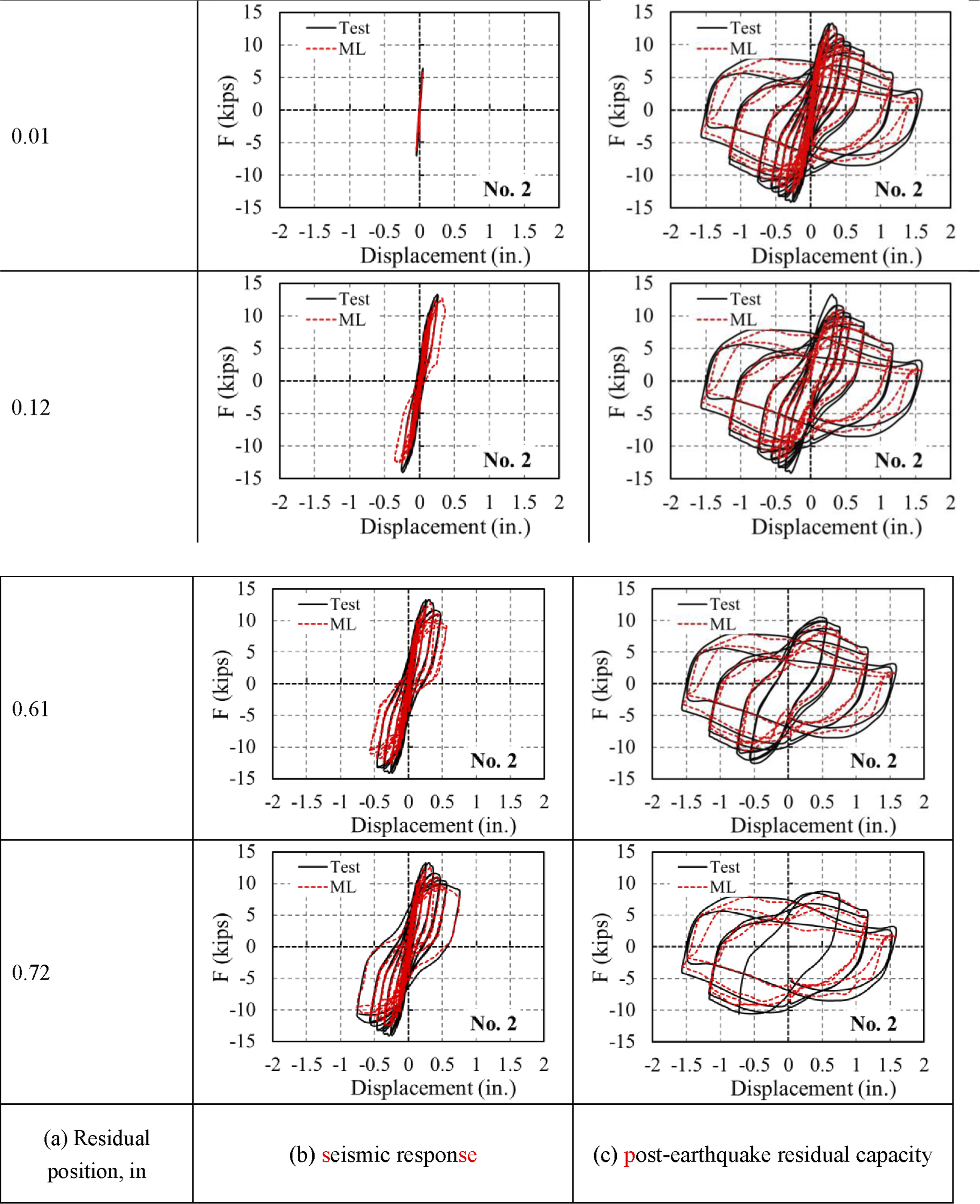

At small residual displacement, the predicted reloading segments coincide with experiments, indicating that the model captures the elastic-to-mild damage regime. As residual displacement increases, slight conservative bias appears: the predictor underestimates reloading strength and over-smooths pinching, consistent with the higher prevalence of spalling, bar buckling, and bond degradation at these states. Such states are also rarer in the training set, so the sequence model regularizes toward smoother trajectories. Taken together, the discrepancies are physically plausible and concentrate at severe-damage tails; they do not alter the correct ranking of capacity across residual-drift levels.

Case study

Cyclic loading test

Five full-scale RC columns were tested under constant axial load with lateral cyclic loading, shown in Figure 17. All columns shared the same geometry: square section 13.8 in × 13.8 in, clear cover 0.98 in, height 37.4 in (shear-span ratio ≈3). Each column had 12 longitudinal bars of 0.63 in diameter, giving a longitudinal reinforcement ratio ρ ≈ 1.97%. Transverse reinforcement was arranged as closed hoops of 0.31 in diameter at a uniform spacing of 2.76 in, corresponding to ρv ≈ 1.91%. The design of the RCC specimens met the requirements of JGJ3-2010, 2010.

Figure 17.

Geometric configuration and reinforcement details of full-scale RCC specimens.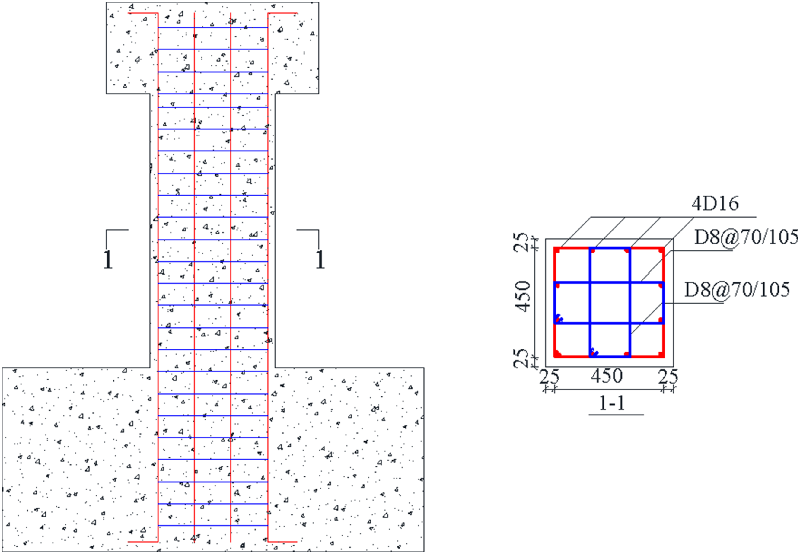

The variables across the five specimens were axial load level and reinforcement grade. Axial loads N (kips) were 16.9 for C1–C3, 33.8 for C4, and 42.3 for C5. Longitudinal steel grades were HRB400 (C1–C2) and HRB600 (C3–C5); stirrup steel was HRB400 in C1 and HRB600 in C2–C5. All columns were cast in a single batch. Six standard cubes (150 mm ≈ 5.9 in) were prepared; the average cube strength was 6873 psi (GB 50081-2016, 2016), and the code-converted axial compressive strength was 4452 psi. Rebar tensile properties were obtained per GB/T 228.1-2010, 2011.

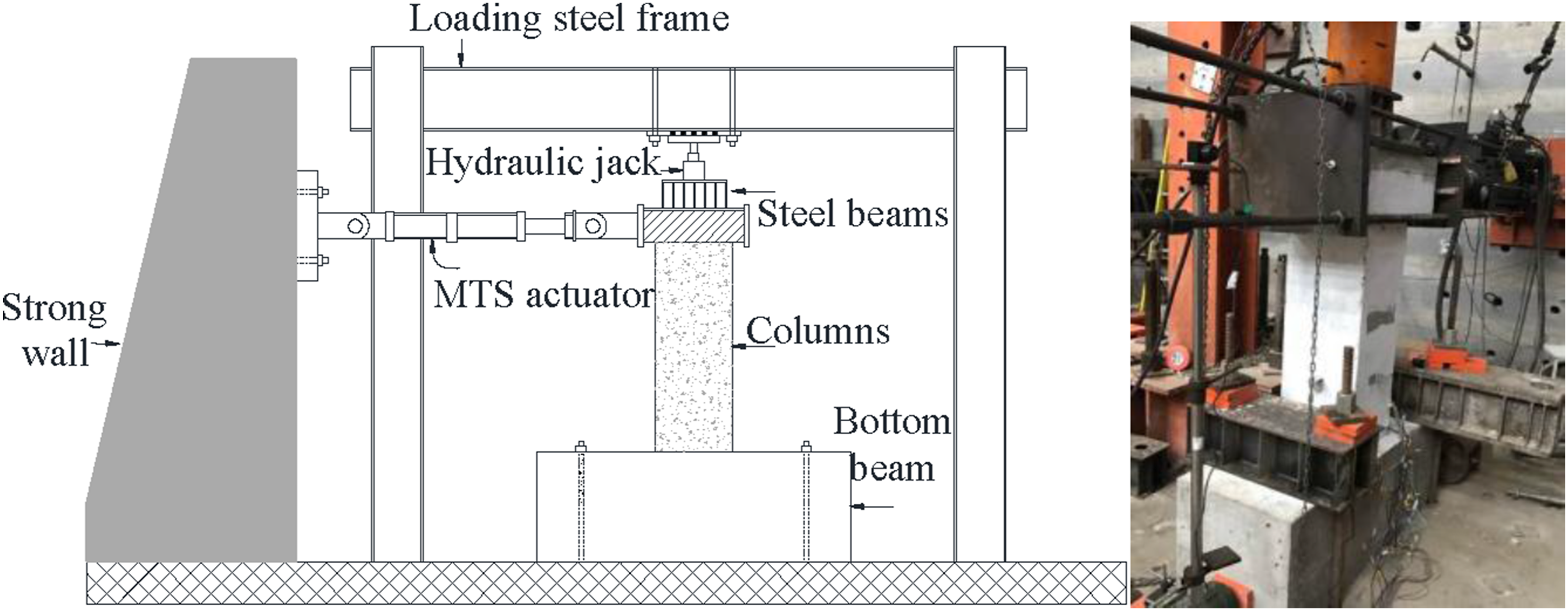
A cantilever setup was used (Figure 18). A hydraulic jack applied the preset constant axial load at the column top; an MTS actuator imposed the lateral cyclic history. The protocol followed the Chinese seismic test specification JGJ/T 101-2015, 2015.

Force-control before yielding, with 6.75 kips per stage (one cycle each).

Displacement-control after yielding; each amplitude increment equaled the yield displacement; three cycles per amplitude.

Termination when lateral resistance dropped below 85% of peak or bar fracture occurred.

Figure 18.

Experimental setup for cyclic loading tests of RCC specimens.

All columns showed pinching, progressive stiffness/strength degradation, and post-peak descending branches with increasing displacement (Figure 19), consistent with shear slip, cracking/crushing, and steel yielding. These records form the experimental basis for the subsequent theoretical, FE, and ML analyses (see also related discussion in Ni et al., 2022).

Figure 19.

Experimental lateral force–displacement hysteresis of RC columns C1–C5.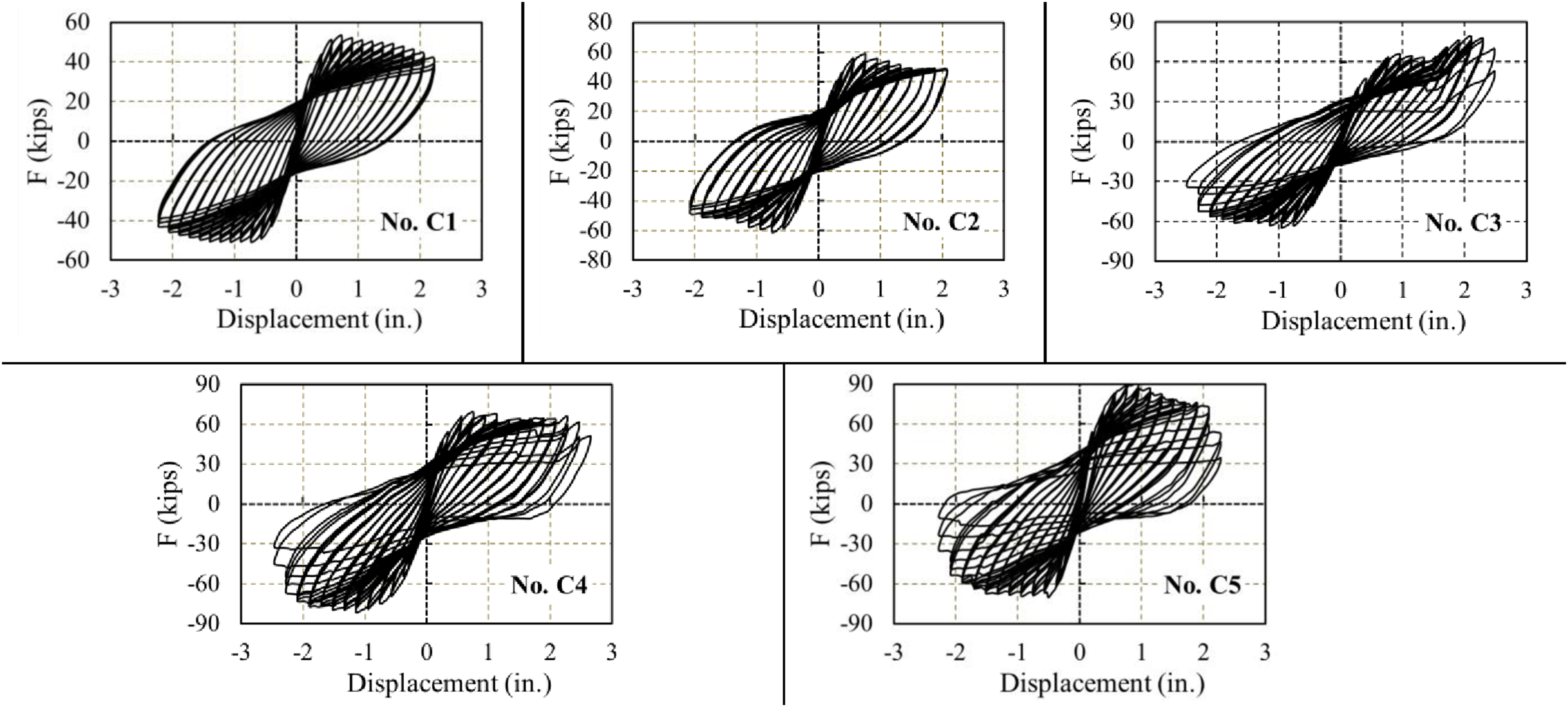

Damage curves and residual seismic performance

Damage curves

Substitute the size, reinforcement, axial load and other information of each specimen into the above ML-Pd to obtain the peak deformation of the RCC under different residual displacements (different earthquake conditions), and then substitute the characteristics of the RCC into the ML-Dc to predict the deformation capacity of each specimen under low-cycle repeated loads. Substituting into equation (1), the predicted damage curve of each RCC can be calculated. Figure 20 demonstrates the comparison of the test and predicted damage curves of the RCCs. Overall, the proposed prediction method based on the ML- Pd and ML-Dc models can more effectively capture the damage evolution law of each specimen under low-cycle repeated loads. The prediction curves of all specimens match well the overall trend of the test curves. From the perspective of local fitting effect, the prediction curves of specimens C1, C2 and C3 are highly consistent with the test curves throughout the loading history, and the model is more accurate in predicting the maximum damage position and its corresponding displacement. The C4 specimen is slightly underestimated in the negative residual displacement area, but the positive part is well fitted, indicating that the model still has strong adaptability when dealing with asymmetric loading paths. For the C5 specimen, the damage of the model in the positive unloading stage is slightly conservatively predicted, but the overall trend is consistent with the experiment. In summary, the damage prediction method based on ML proposed in this study demonstrates strong fitting performance and high prediction accuracy under different specimens, and has the potential to be promoted and applied in actual engineering.

Figure 20.

Damage curves of each RCC specimen.

RSC evaluation

The comparison of the post-seismic RSC of the RCC specimens under different residual displacements dr is presented in Figure 21. The red one is the curve obtained from the test, and the black one is the hysteresis response curve predicted by the above ML model. Combined with the actual dr of the specimen, the corresponding peak deformation Pr can be obtained through the ML-Pd model prediction. From Figure 21, the proposed ML-Hc model can well restore the full process of hysteresis response of the RCC specimen under different post-seismic residual displacements. The predicted curves are in strong agreement with the test results in terms of the shape of the hysteresis loop, stiffness degradation, strength degradation and residual deformation, reflecting the strong ability of the model in fitting nonlinear path-dependent loading behavior. With the increase of dr, the post-seismic hysteresis curve of the RCC demonstrates obvious strength deterioration and stiffness degradation, and the cycle area gradually decreases, reflecting the decrease in the energy dissipation capacity of the RCC under earthquake action. The model can accurately reflect this degradation process, especially in the large deformation stage (such as dr > 1) can still well reproduce the unloading path and residual strength characteristics in the test, indicating that it has strong potential in the assessment of post-earthquake residual bearing capacity.

Figure 21.

Predicted vs. experimental post-earthquake RSC curves for RCCs under different residual displacements.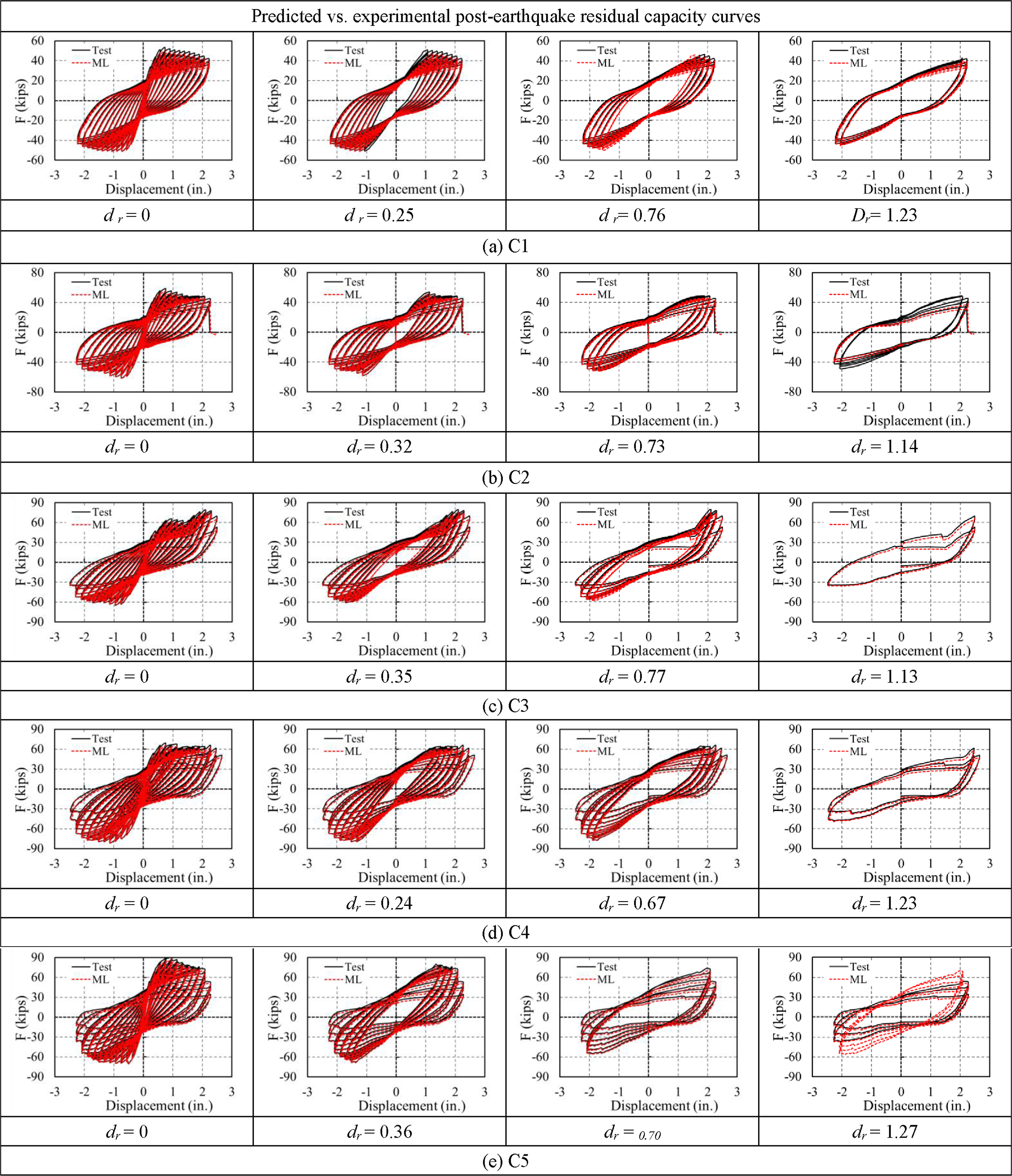

Conclusion

This study builds a residual-drift–based framework for post-earthquake RSC assessment of RCCs. A measured residual drift is used to (i) infer the peak deformation that was reached (ML-Pd), (ii) estimate deformation capacity under cyclic loading (ML-Dc), and (iii) generate full hysteresis sequences from peak to failure (ML-Hc). The main findings are.

(1) Model performance on the 326-specimen database. Using the NEES–ACI 369 records, tree-boosting models (XGBoost) give high accuracy for peak- and capacity-type targets (test R² ≥ 0.94), while an LSTM (32 units) reproduces force–displacement sequences with R² ≈ 0.99 on the hold-out set. All models were evaluated under a fixed train–test split with uniform preprocessing.

(2) Damage quantification from residual drift. Residual drift shows a clear nonlinear link to damage level: the damage index rises to a peak near the maximum residual drift and then attenuates. Predicted damage–drift curves match the experimental trend and turning points, allowing straightforward grading after earthquakes.

(3) RSC estimation. Chaining ML-Pd → ML-Hc reconstructs the post-peak response and yields residual seismic capacity (RSC). For representative hold-out specimens, predicted loops agree with tests in envelope, pinching, and stiffness/strength degradation; the backbone capacity is captured within the experimental trend.

(4) Experimental verification. Five full-scale cyclic tests (constant axial load, lateral cycling) exhibit the same features—pinching and progressive degradation. The framework reproduces these behaviors and the reloading curves at prescribed residual drifts, supporting rapid, quantitative assessment for repair/strengthening decisions.

Limitations, scope, and applicability

The models were trained and validated on published quasi-static cyclic tests of RCCs; direct use for other member types or markedly different boundary/loading conditions has not been verified. Performance depends on the quality and coverage of the compiled database; measurement and reporting variability may carry over to the predictions. High-drift states are less frequent, and the sequence model smooths cycle-to-cycle deterioration, which may understate abrupt degradation. Predictions outside the training ranges are not assured and should be interpreted with engineering judgment and code checks. Our corpus includes shear-dominated columns (low a/d, limited confinement, diagonal-tension/web-crushing), and the models were trained and evaluated including these specimens; within this covered range the framework reproduces key hysteretic features—strength, stiffness degradation, and pinching—so it is applicable to shear-dominated columns. In the training database, shear-dominated specimens account for 40 out of 326 tests (12.3%), providing direct training coverage for this failure mode. Nevertheless, because this subset is comparatively smaller than the flexural-dominated subset, predictions for extreme shear-critical cases should be interpreted with caution. Future work will further expand the shear-critical subset to enhance robustness. In addition, shear-related indicators (e.g., a/d, transverse-reinforcement index, axial–shear demand) will be incorporated, a failure-mode classifier will be introduced to route predictions, and uncertainty/out-of-distribution (OOD) diagnostics will be reported to flag inputs outside the training domain.

Overall, the residual-drift–based workflow provides a practical path from a measurable post-event quantity to damage grading, hysteresis reconstruction, and residual capacity, enabling fast and reproducible post-earthquake decisions for RC columns.

Footnotes

ORCID iDs

Ni Xiangyong

Chen Yuxin

Xu Jiaqi

Funding

The authors disclosed receipt of the following financial support for the research, authorship, and/or publication of this article: This work was supported by the Shanghai Young Scientific Talents “Sailing” Program (Grant No. 23YF1418800), Shanghai Pujiang Program (Grant No. 24PJD136) and National Natural Science Foundation of China (Grant No. 52308523).

Declaration of conflicting interests

The authors declared no potential conflicts of interest with respect to the research, authorship, and/or publication of this article.

Data Availability Statement

Data are presented in the open experimental NEES: ACI 369 rectangular column database.*

References

Akbari

Khanmohammadi

(2021) Prediction of residual and maximum displacement of concrete bridge columns under near-field motions using integrated experimental simulation data and distributed plasticity approaches. Journal of Structural Engineering 147(12): 04021199. https://doi.org/10.1061/(asce)st.1943-541x.0003172

Azhari

Jamshidian

Hamidia

(2025) AI-driven computer vision-based automated repair activity identification for seismically damaged RCCs. Automation in Construction 170: 105959. https://doi.org/10.1016/j.autcon.2024.105959

Dong

Qiang

Canxing

, et al. (2022) Residual displacement responses of structures subjected to near-fault pulse-like ground motions. Structure and Infrastructure Engineering 18(3): 313–329. https://doi.org/10.1080/15732479.2020.1835997

Dong

Sun

Hongnan

, et al. (2023) Analysis on residual displacement of reinforced concrete bridge piers standing in liquefiable field. Engineering Mechanics 40(10): 154–168.

Dong

Wang

Han

, et al. (2024) Re-centering capability of partially self-centering structures with flag-shaped hysteretic behavior subjected to near-fault pulsed ground motion. Soil Dynamics and Earthquake Engineering 186: 108892. https://doi.org/10.1016/j.soildyn.2024.108892

Feng

Gong

(2020) Investigation on residual displacements for SDOF systems with various initial viscous damping models. Structures 28: 1831–1844. https://doi.org/10.1016/j.istruc.2020.10.018

Gang

Tong

(2025) Advances in AI-powered civil engineering throughout the entire lifecycle. Advances in Structural Engineering 28(9): 1515–1541.

Gang

Tong

Aiqun

, et al. (2023) Development and investigation of a self-centering cable brace with variable slip stiffness for braced frame structure. Journal of Building Engineering 76: 107383.

GB 50081-2016 (2016) Code for Design of Concrete Structures. Beijing, China: China Architecture & Building Press.

10.

GB/T 228.1-2010 (2011) Metallic materials-tensile testing-part 1: Method of Test at Room Temperature. Beijing (China): Standards Press of China.

11.

Ghannoum

Pujol

Christine

, et al. (2015) NEES: ACI 369 Rectangular Column Database. Berkeley,CA: Univ. of California. https://doi.org/10.4231/D36688J50

12.

Graves

Schmidhuber

(2005) Framewise phoneme classification with bidirectional LSTM and other neural network architectures. Neural Networks 18(5): 602–610. https://doi.org/10.1016/j.neunet.2005.06.042

13.

Greff

Srivastava

Koutník

, et al. (2017) LSTM: a search-space odyssey. IEEE Transactions on Neural Networks and Learning Systems 28(10): 2222–2232. https://doi.org/10.1109/TNNLS.2016.2582924

14.

Han

Xiao

Tan

, et al. (2025) Experimental study and analytical model of full-scale concrete columns with hybrid steel-FRP reinforcements under axial compression and cyclic lateral loading. Engineering Structures 336: 120301. https://doi.org/10.1016/j.engstruct.2025.120301

15.

Zhu

Wang

(2022) Machine learning-driven probabilistic residual displacement-based design method for improving post-earthquake repair ability of steel moment-resisting frames using self-centering braces. Journal of Building Engineering 61: 105225. https://doi.org/10.1016/j.jobe.2022.105225

16.

Jamshidian

Hamidia

(2023) post-earthquake damage assessment for RCCs using crack image complexity measures. Bulletin of Earthquake Engineering 21: 6029–6063. https://doi.org/10.1007/s10518-023-01745-4

17.

JGJ/T 101-2015 (2015) Specification for Seismic Test of Buildings. Beijing: China Architecture & Building Press.

18.

JGJ3-2010 (2010) Technical Specification for Concrete Structures of Tall Building. Beijing, China: China Architecture & Building Press.

19.

Jianbing

Gang

(2013a) Correlation analysis between residual deformation response of SDOF system and earthquake intensity index. China Civil Engineering Journal 46(06): 1–7.

20.

Jianbing

Gang

(2013b) Study on iso-strength residual displacement spectrum of single degree of freedom system. China Civil Engineering Journal 46(10): 82–88.

21.

Katsimpini

(2025) Maximum seismic displacement assessment of composite steel-concrete structures from residual deformations. Bulletin of Earthquake Engineering 23(6): 1–22. https://doi.org/10.1007/s10518-025-02152-7

22.

Kawashima

Macrae

Hoshikuma

, et al. (1998) Residual displacement response spectrum. Journal of Structural Engineering 124(5): 523–530. https://doi.org/10.1061/(asce)0733-9445(1998)124:5(523)

23.

Lai

Jiang

(2023) Mapping between the residual deformation in the CRTS II slab track-bridge system and the rail deformation under earthquake in the transverse direction. China Civil Engineering Journal 56(06): 87–99.

24.

Zhang

(2021) Research on the physical inter-story drift ratio and the damage evaluation of RC shear wall structures. Earthquake Engineering and Engineering Vibration 20(4): 753–766. https://doi.org/10.1007/s11803-021-2054-6. https://doi.org/10.1007/s11803-021-2054-6

25.

Luo

Wang

, et al. (2020) Numerical model for the residual seismic capacity of seismically damaged reinforced concrete columns. Engineering Mechanics 37(12): 52–67.

26.

Chen

Wang

(2023) Evaluation of the residual seismic capacity of post-earthquake damaged RC columns based on the damage distribution model. Buildings 13(3): 595. https://doi.org/10.3390/buildings13030595

27.

Liepa

Blaževičius

Merkevičiūtė

, et al. (2016) Structural shakedown: a new methodology for estimating the residual displacements. Journal of Civil Engineering and Management 22(8): 1055–1065. https://doi.org/10.3846/13923730.2016.1217924

28.

Liu

Xiao-wei

Yi-xiao

(2022) Analysis of the seismic liquefaction of caisson wharves under strong earthquakes using the ALE method. Engineering Mechanics 39(5): 177–187.

29.

Liu

Cheng

(2025) Influence of ground motion duration on the residual displacement spectrum of structures. Journal of Vibration and Shock 44(14): 139–148.

30.

Maeda

Kang

(2009) post-earthquake damage evaluation of reinforced concrete buildings. Journal of Advanced Concrete Technology 7(3): 327–335. https://doi.org/10.3151/jact.7.327

31.

Mahin

Moehle

(2024) Probabilistic assessment of global damage index for steel moment frames. Journal of Structural Control and Health Monitoring* 31(1): e3065. https://doi.org/10.1002/stc.3065

32.

Qiang

(2022) Cyclic test and numerical analysis of the seismic performance of concrete columns reinforced by HRB600 steel bars. Journal of Building Engineering 50: 104211. https://doi.org/10.1016/j.jobe.2022.104211

33.

Pang

Yuan

Liu

, et al. (2026) Flexural behavior of steel beams with double corrugated webs: experimental and analytical investigations. Thin-Walled Structures 218: 113929. https://doi.org/10.1016/j.tws.2025.113929

34.

Park

Ang

AH-S

Wen

(1985) Seismic damage analysis of reinforced concrete buildings. Journal of Structural Engineering 111(4): 740–757. https://doi.org/10.1061/(asce)0733-9445(1985)111:4(740)

35.

Ruiz‐ García

Miranda

(2006) Residual displacement ratios for assessment of existing structures. Earthquake Engineering & Structural Dynamics 35(3): 315–336. https://doi.org/10.1002/eqe.523

36.

Shan

Liu

Ouyang

(2021) Residual-based damage evaluation of RCCs using feature classification and model optimization. The Structural Design of Tall and Special Buildings 30(15): e1887. https://doi.org/10.1002/tal.1887

37.

Shan

Zhang

Liu

, et al. (2024) Deformation prediction of large-scale civil structures using spatiotemporal clustering and empirical mode decomposition-based long short-term memory network. Automation in Construction 158: 105222. https://doi.org/10.1016/j.autcon.2023.105222

38.

Shturmin

Lee

Choi

, et al. (2024) Machine learning-based residual drift prediction of concrete-filled steel tube columns under earthquake loads. Journal of Building Engineering 97: 110903. https://doi.org/10.1016/j.jobe.2024.110903

39.

Sun

Hua

Jin

, et al. (2016) Numerical seismic analysis model for reinforced concrete bridge piers based on OpenSees. World Earthquake Engineering 32(1): 266–276.

40.

Wang

Yuhuan

(2024) Study on residual displacement model and restoring force model of core walls. Earthquake Resistance and Retrofitting Engineering 46(04): 1–11.

41.

Yazgan

Dazio

(2011) The use of post-earthquake residual displacements as a performance indicator in seismic assessment. Georisk: Assessment and Management of Risk for Engineered Systems and Geohazards 5(1): 59–76. https://doi.org/10.1080/17499511003679964

42.

Zeng

Zhuo

Wang

(2021) Influence factors analysis and Bayesian estimation for residual displacement index of RC pier. Journal of Vibration and Shock 40(19): 145–150.

43.

Zhang

Wang

(2023) Probabilistic residual displacement-based design for enhancing seismic resilience of BRBFs using self-centering braces. Engineering Structures 295: 116808. https://doi.org/10.1016/j.engstruct.2023.116808

44.

Zhang

Reuland

Shan

, et al. (2024) Post-earthquake structural damage assessment and damage state evaluation for RC structures with experimental validation. Engineering Structures 304: 117591. https://doi.org/10.1016/j.engstruct.2024.117591

45.

Zhao

Yan

Liu

, et al. (2021) Seismic damage assessment of reinforced concrete (RC) pier columns based on residual drift in saline soil environment. Journal of Earthquake Engineering 26(15): 8000–8020. https://doi.org/10.1080/13632469.2021.1984343

46.

Zheng

Chuanhe

Jia

, et al. (2023) Application overview of artificial intelligence technology in bridge seismic field. Earthquake Engineering and Engineering Dynamics 43(4): 1–13.

47.

Zhong

Wei

Shao

, et al. (2024) An efficient method for predicting the residual displacement of UBPRC columns under near-fault ground motions. Journal of Earthquake Engineering 28(5): 1451–1473. https://doi.org/10.1080/13632469.2023.2234500

48.

Zhou

Shahria Alam

Song

, et al. (2022) Probability -based residual displacement estimation of unbounded laminated rubber bearing supported highway bridges retrofitted with transverse steel damper. Engineering Structures 272: 115053. https://doi.org/10.1016/j.engstruct.2022.115053