Simulation and analysis of girder end longitudinal motion for suspension bridges considering multiple resistances using on-site vehicle load sequences

Abstract

Under repeated girder end displacements, various forms of damage and deterioration occur in the girder end restraining devices, leading to their premature failure. To understand the inner law of the longitudinal girder end motion, a model development and updating method is proposed for suspension bridges considering multiple types of restraints by using on-site vehicle load sequences. In addition, key parameters associated with the longitudinal girder end motion are discussed based on the updated model. First, the on-site vehicle load sequences are generated based on the vehicle weighing and video systems, and the corresponding input loads for numerical simulation are obtained using the virtual work principle and shape functions. Then, an initial finite element model of a suspension bridge is developed considering the resistances of the expansion joints etc. Transient dynamic analysis is used to calculate the time history of the girder end displacement under the on-site vehicle load sequences. Subsequently, the longitudinal resistance parameters, for example, the spring stiffness, are selected as optimized variables, where the genetic algorithm is used to achieve the optimal values. Finally, the characteristics of the displacement at the girder end are examined in the context of the varying volume of traffic and proportions of heavy vehicles using the updated finite element model. As a result, the optimal spring stiffness, damping coefficient, and frictional force are 14,563.5 kN/m, 654,371 $N \cdot S \cdot m^{- 1}$ and 0.0330256, respectively. Simulation results reveal that increases in both traffic volume and heavy vehicle proportion lead to greater cumulative girder end displacements, with the latter playing a dominant role in amplifying displacement magnitudes.

Keywords

suspension bridges girder end displacement girder end restraints on-site vehicle load sequences transient dynamic analysis

Introduction

Suspension bridges, typically characterized by full-floating or semi-floating structural systems, are prone to longitudinal motion under temperature variations, wind loads, and vehicular loads. The repeated longitudinal displacement at girder ends imposes significant demands on bridge restraints, including expansion joints, dampers, and bearings, which may result in excessive wear, deterioration, and even premature functional failure during service. For instance, the expansion joints of the Runyang Suspension Bridge and the bearings of the Jiangyin Bridge failed within only a few years of operation due to frequent and unpredictable girder movements (Guo et al., 2015), while the bearings of the Humber Bridge experienced severe wear caused by repeated longitudinal motion at girder ends (Brownjohn et al., 2020). Such failures not only compromise ride comfort and structural safety, but also lead to costly maintenance and traffic disruptions. Therefore, a clear understanding of the longitudinal motion characteristics at girder ends is essential for evaluating the service performance and durability of restraint systems, improving maintenance strategies, and providing guidance for the design and optimization of bridge restraint devices in long-span suspension bridges.

With the assistance of structural health monitoring systems, field monitored girder end longitudinal displacements are recorded. Based on these field measured data, an increasing volume of research has emerged. A variety of methodologies, including regression models, wavelet transforms, and Bayesian models, have been utilized to elucidate the correlation between temperatures and girder end displacements (Ni et al., 2020; Ren et al., 2022; Xu et al., 2010). Consequently, a robust linear correlation is observed between temperatures and girder end displacements, with the former significantly contributing to the large amplitude of girder end displacement signals. Furthermore, to improve the accuracy of thermal response estimation and to mitigate the time-lag effect, deep learning methods were used to predict temperature-induced girder end displacements (Jin et al., 2025; Sun et al., 2023c). This correlation has facilitated extensive research in the areas of condition assessment, damage diagnosis, and anomaly detection for suspension bridges (Ni et al., 2007, 2020; Ren et al., 2022; Wu et al., 2021).

Early studies on traffic loading mainly adopted simplified vehicle platoon models or code-based equivalent lane loads. However, such approaches are unable to accurately capture the stochastic characteristics of real traffic flow, including variations in vehicle weight, speed, spacing, and vehicle composition. With the rapid development of weigh-in-motion (WIM) systems and traffic monitoring technologies, data-driven stochastic traffic flow simulation methods based on measured traffic information have become increasingly popular. In these studies, probabilistic and statistical approaches are commonly employed to establish distributions of vehicle parameters, while Monte Carlo simulation, stochastic process theory, and vehicle arrival models are used to generate continuous random traffic streams (Wang and Xu, 2019; Xu et al., 2021, 2023b). These methods provide a more realistic representation of bridge responses under operational traffic conditions.

When subjected to stochastic vehicle loads, the girder end displacement signal exhibits a high frequency and small amplitude characteristic, leading to significant cumulative girder end displacements. The magnitude of this cumulative displacement is a critical determinant in the failure mechanism of the restraints (Guo et al., 2015). In an effort to counteract undesirable cumulative displacements, a range of restraints, such as dampers, have been recommended to regulate the reciprocating longitudinal motion in long-span suspension bridges (Guo et al., 2016; Jing et al., 2024a; Sun et al., 2023a; Xu et al., 2023). Furthermore, the cumulative displacement was utilized as a metric to identify damper failure and forecast the service lifespan of sliding bearings (Li et al., 2020; Sun et al., 2023b; Sun et al., 2023b, 2023b; Xu et al., 2023a; Yang et al., 2024).

Numerical simulation is one of the most critical methods in studying longitudinal motion at girder ends for suspension bridges. Longitudinal resistances were modeled by using various types of elements in previous studies. Command CP and spring elements in ANSYS were used to model resistances at girder ends (Huang et al., 2023; Jing et al., 2024b; Xu et al., 2023). This approach has relatively high computational efficiency, but it typically assumes a linear resistance behavior, thereby neglecting nonlinear effects such as expansion joint slip, bearing friction, and damping forces. To consider various non-linear resistances, COMBIN37 and COMBIN39 in ANSYS were used to simulate the constraints of expansion joints, bearings and dampers (Dong et al., 2024; Feng et al., 2025; Gao et al., 2022; Guo et al., 2015, 2016; Li et al., 2020; Qu et al., 2023; Wang et al., 2024, 2025; Wu et al., 2024; Xia et al., 2020; Yang et al., 2024). This approach can, to some extent, account for nonlinear effects such as frictional sliding, gap closure, and contact separation, thereby improving the accuracy of longitudinal response analysis at girder ends. In addition, considering the complexity of longitudinal constraint sources in real bridge systems, previous studies have commonly adopted an “equivalent spring” to uniformly represent the longitudinal boundary condition of bridges. This equivalent spring is generally used to integrate the variable stiffness behavior of shear springs at expansion joints, the additional constraint effects from pinned connections at hanger or cable anchorage locations, and other structural components contributing to longitudinal resistance. Therefore, its stiffness does not correspond to the physical stiffness of a single component, but rather reflects a system-level equivalent parameter resulting from the combined action of multiple mechanisms, exhibiting a clear system equivalence. However, the selection basis and parameter rationality of this equivalent spring stiffness have not been clearly clarified in existing studies.

Model updating is a key procedure in numerical simulation and is particularly important for finite element analysis of longitudinal girder end motion in suspension bridges. Existing studies mainly adopt three categories of updating approaches. The first category relies on modal parameters (e.g., natural frequencies and mode shapes) for model calibration (Wu et al., 2024; Xu et al., 2023). However, because longitudinal stiffness, damping, and friction have limited influence on global modal characteristics, this approach is insufficient to accurately capture the local longitudinal boundary behavior, which may lead to errors in displacement prediction. The second category is based on vertical dynamic responses, where transient analysis results such as vertical displacement or girder deflection time histories are used for parameter identification (Wang et al., 2024, 2025). Nevertheless, due to the significant difference between vertical and longitudinal force mechanisms, parameters calibrated in the vertical direction cannot guarantee reliable representation of longitudinal boundary conditions. The third category uses static loading test results by matching simulated and measured girder end displacements to update model parameters (Dong et al., 2024; Li et al., 2020; Xia et al., 2020; Yang et al., 2024). However, this approach is limited in identifying dynamic parameters such as damping and friction. Overall, all existing methods have certain limitations and cannot simultaneously and accurately capture key longitudinal effects such as stiffness, damping, and friction. Therefore, transient dynamic analysis based on girder end displacement time histories is necessary to achieve more reliable identification of longitudinal resistance parameters and improved model updating accuracy.

This study proposes a numerical simulation method to model the longitudinal motion of girder ends, taking the constraints at the girder ends into account. First, on-site vehicle load sequences are generated based on measured vehicle load data. Subsequently, an initial finite element model of the suspension bridge is established, incorporating spring, damping, and friction elements. The optimal values of the longitudinal constraint parameters, namely spring stiffness, damping coefficient, and friction coefficient, are then determined using genetic algorithm (GA) by minimizing the discrepancies between the simulated and measured displacement time histories. Finally, the characteristics of the girder end displacements are examined in the context of varying traffic volumes and proportions of heavy vehicles using the updated finite element model.

The studied bridge and its monitoring system

General information

The Huangpu Bridge, which spans the primary channel of the Zhujiang River, serves as a vital connection between the Huangpu and Panyu districts in Guangzhou. The total length of the bridge extends to 7049 m, featuring an innovative hybrid design that seamlessly integrates both a suspension and a cable-stayed bridge. This research primarily concentrates on the suspension component of the bridge. The span configuration is (290 + 1108 + 350) meters, with a standard suspension spacing of 12.8 m, as illustrated in Figure 1. The suspender wire rope has a nominal diameter of ϕ 56 mm and a nominal tensile strength of 1770 MPa. The main cables of the Huangpu Bridge are constructed from prefabricated parallel wire strands. Each main cable comprises 147 through-length strands, each of which is made up of 127 high-strength galvanized steel wires. These wires have a diameter of 5.20 mm and a nominal tensile strength of 1670 MPa.

Figure 1.

Front view of the studied suspension bridge.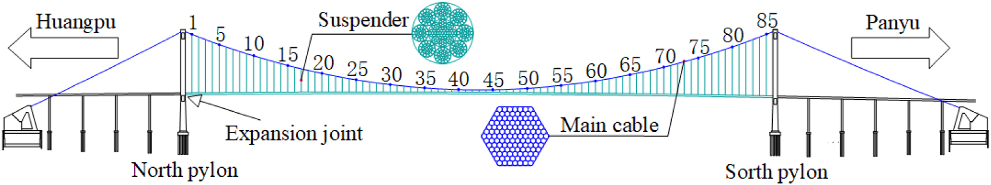

Girder end restraint devices of the Huangpu Bridge consist of vertical bearings, viscous dampers, and expansion joints, as illustrated in Figure 2. The vertical bearings utilize a roller bearing design with a rated capacity of 4900 kN. Viscous dampers, possessing a rated damping force of 2 MN, serve to connect the bearing pad stone and the steel box girder. The expansion joints facilitate the connection between the main span and the approach.

Figure 2.

Structural configurations of the three girder end restraints.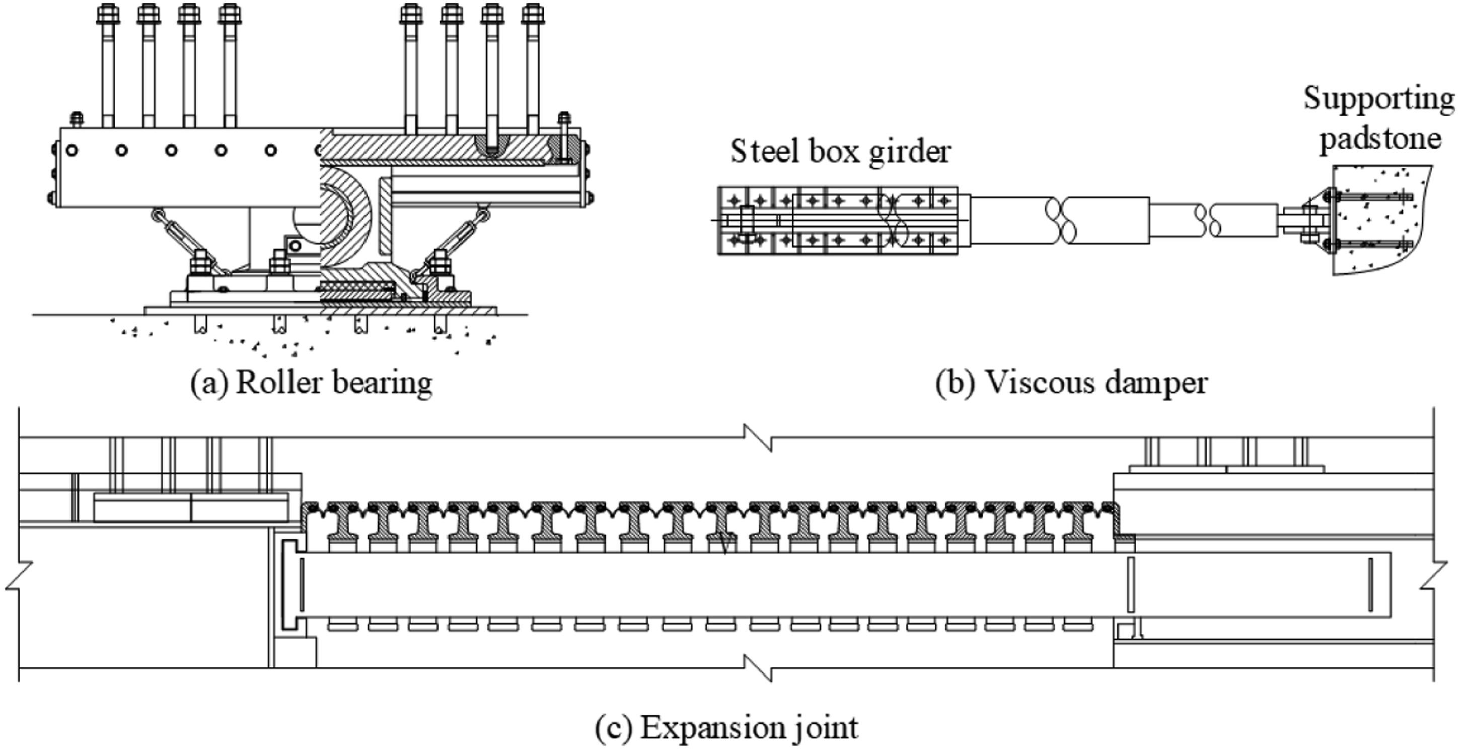

Bridge monitoring system

The suspension bridge is equipped with an advanced monitoring system, incorporating a variety of sensors to monitor environmental factors, external loads, structural response, and variations. In addition, short-term monitoring systems are frequently employed to gather more dependable data for the calibration of long-term monitoring information.

Six cameras are strategically positioned at the entrance, mid-span, and exit of the bridge deck to capture vehicle data - Figure 3. The arrival time of each vehicle is logged by the cameras located at the entrance. Leveraging embedded algorithms within the cameras, vehicle license plates and carriageways are automatically identified.

Figure 3.

Camera arrangement on the bridge deck.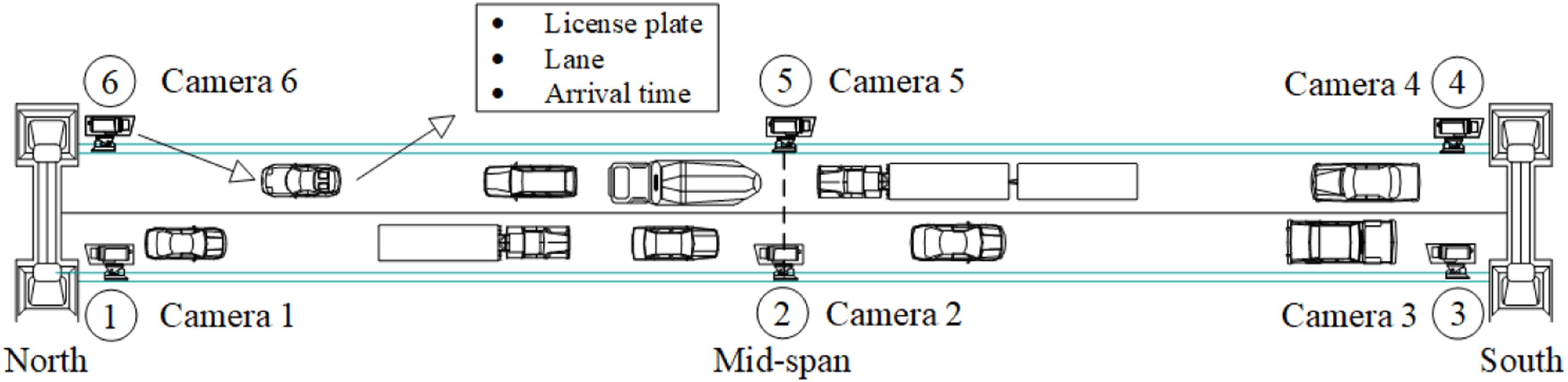

In real traffic flow, acceleration and deceleration behaviors of individual vehicles are highly stochastic and difficult to reproduce accurately in the absence of detailed trajectory data, making it challenging to model them reliably at the engineering scale. Besides, for highway bridges considered in this study, vehicles generally maintain relatively stable speeds while passing through the main span, with limited variations in velocity. Therefore, as illustrated in Figure 4, a piecewise constant speed assumption is employed to represent vehicle velocities, which helps reduce measurement errors to a certain extent. In addition, on-site surveillance videos are used to cross-check the traffic flow, enabling the identification and supplementation of any potentially missing vehicles, thereby improving the completeness and accuracy of the load inputs.

Figure 4.

Illustration of vehicle speed calculation.

The toll booths are equipped with a weigh-in-motion (WIM) system to collect axle configuration and vehicle weight data, as shown in Figure 5. Since both the toll booth system and deck camera monitoring system record license plate information, the two databases can be linked through the license plate number. The integrated database therefore contains vehicle type, arrival time, vehicle weight, carriageway, and vehicle speed information.

Figure 5.

Connection of the database at the toll booth and bridge deck.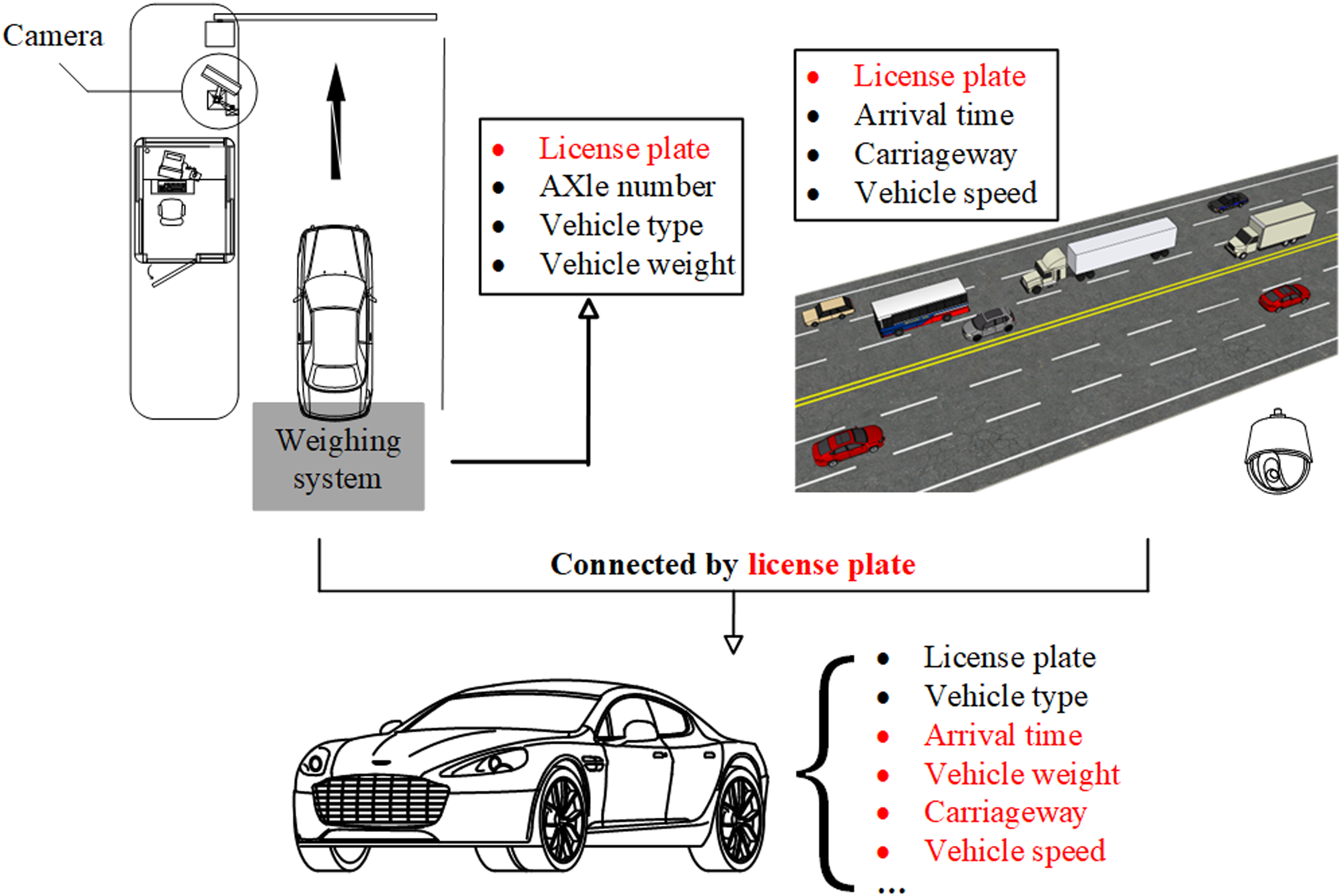

A pull-rope sensor with a sampling frequency of 20 Hz is installed on the crossbeam to monitor girder end displacement. However, the measured data contain significant noise. Therefore, a push-rod sensor with the same sampling frequency is adopted for short-term monitoring, as shown in Figure 6, due to its higher signal-to-noise ratio. Although the push-rod sensor provides high measurement accuracy, its limited measurement range prevents it from capturing the full seasonal variation of girder end displacement, making it more suitable for short-term monitoring applications. Multiple sensors are arranged near critical measurement points. Through data comparison and fusion, random errors can be effectively reduced, thereby enhancing the accuracy and stability of the measured responses.

Figure 6.

Displacement sensors at the girder end.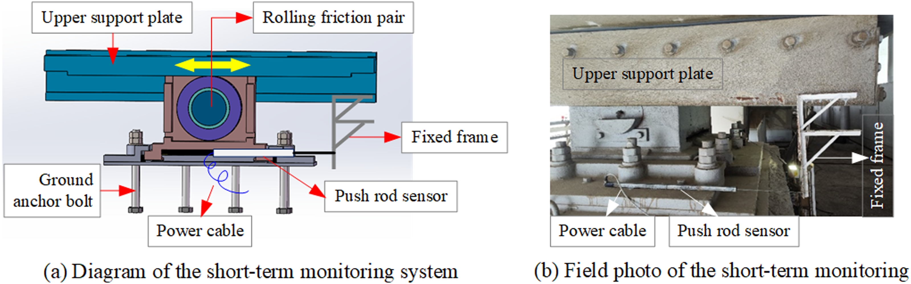

The sensor data also include structural responses induced by temperature loading. However, the vehicle load time history used for subsequent finite element model updating is approximately 100 s. Within this short time window, the variation in ambient temperature is very small (approximately 0.05°C), and the corresponding thermal expansion/contraction-induced displacement is negligible compared with the dynamic response caused by traffic loads. Therefore, from the perspective of engineering accuracy, the influence of temperature effects on the model updating results within this stage is limited and can be reasonably neglected.

Finite element model development and updating

Finite element model development

In this research, a finite element model of the Huangpu Bridge was constructed to emulate the dynamic longitudinal motion of the girder ends under on-site vehicle load sequences. The stiffening girder is represented using the BEAM4 element, which allows for six degrees of freedom at each node. The main cables and suspenders are depicted using LINK10 elements, each offering three degrees of freedom per node. The suspender is connected to the stiffening girder through a rigid beam, which is designed using a material with a high Young’s modulus to ensure minimal deformation.

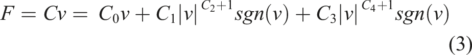
According to the design specifications, to reduce the longitudinal displacement at the ends of the main girders, viscous dampers are installed symmetrically on both sides of the Huangpu Bridge, with two dampers on each side. The damping force provided by the viscous damper is defined as:

F = c {| v |}^{α} s g n (v)

(1)

where c is the damping coefficient, v is the relative velocity and α is the velocity exponent.

The velocity exponent has been calibrated through high-precision experimental testing; therefore, the design value (0.4) is directly employed in the model updating without further optimization to ensure consistency with established engineering practice and physical reliability. It is noted that the velocity exponent may vary under degradation scenarios (e.g., oil leakage). In such cases, or for studies focusing on long-term performance evolution, it can be incorporated as an additional parameter within the model updating framework.

As illustrated in Figure 7, the viscous damper is represented by COMBIN37 element in this model, which consists of a spring and a damper. The element is defined by four nodes, including two active nodes (I and J) responsible for the axial deformation of the spring, and two optional control nodes (K and L). The element’s non-linear behavior, such as damping, is governed by the control nodes in conjunction with the RVMOD function. By specifying appropriate control parameters for the element, the RVMOD function can be utilized to modify the damping coefficient, as follows:

C = C_{0} + C_{1} {| v |}^{C_{2}} + C_{3} {| v |}^{C_{4}}

(2)

F = C v = C_{0} v + C_{1} {| v |}^{C_{2} + 1} s g n (v) + C_{3} {| v |}^{C_{4} + 1} s g n (v)

(3)

where C_i is constant for damping, v represents the relative velocity between the control nodes.

Figure 7.

Finite element model of the studied bridge.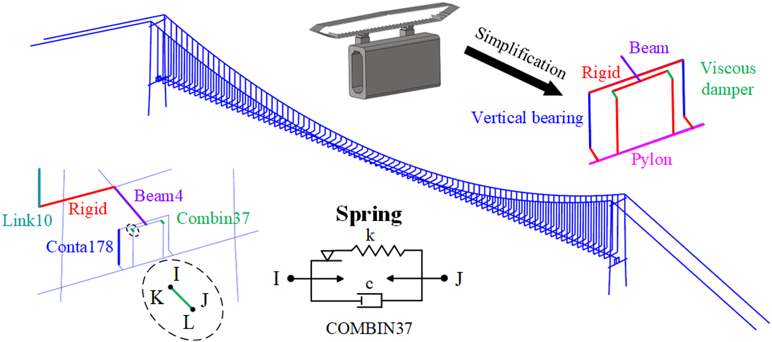

By setting C₀ = C₃ = 0, C₄ = −0.6, the element can be used to simulate a viscous damper. The spring stiffness K and damping coefficient C₁ are determined through GA-based optimization in the subsequent analysis.

Figure 8 presents the displacement time histories recorded by the bearing displacement sensors of the Huangpu Bridge. It can be observed that when the longitudinal displacement direction of the girder reverses, a distinct plateau stage appears in the response, during which the girder end displacement remains approximately constant for a certain period. Previous studies on temperature–displacement relationships have indicated that bearing displacement induced by temperature variation must overcome the maximum static friction force before sliding occurs (Wu et al., 2023). These observations demonstrate that bearing friction is an important factor in accurately simulating girder end displacement and also provides a basis for subsequent studies on bearing degradation and performance evolution.

Figure 8.

Curve of the measured displacement at the girder end.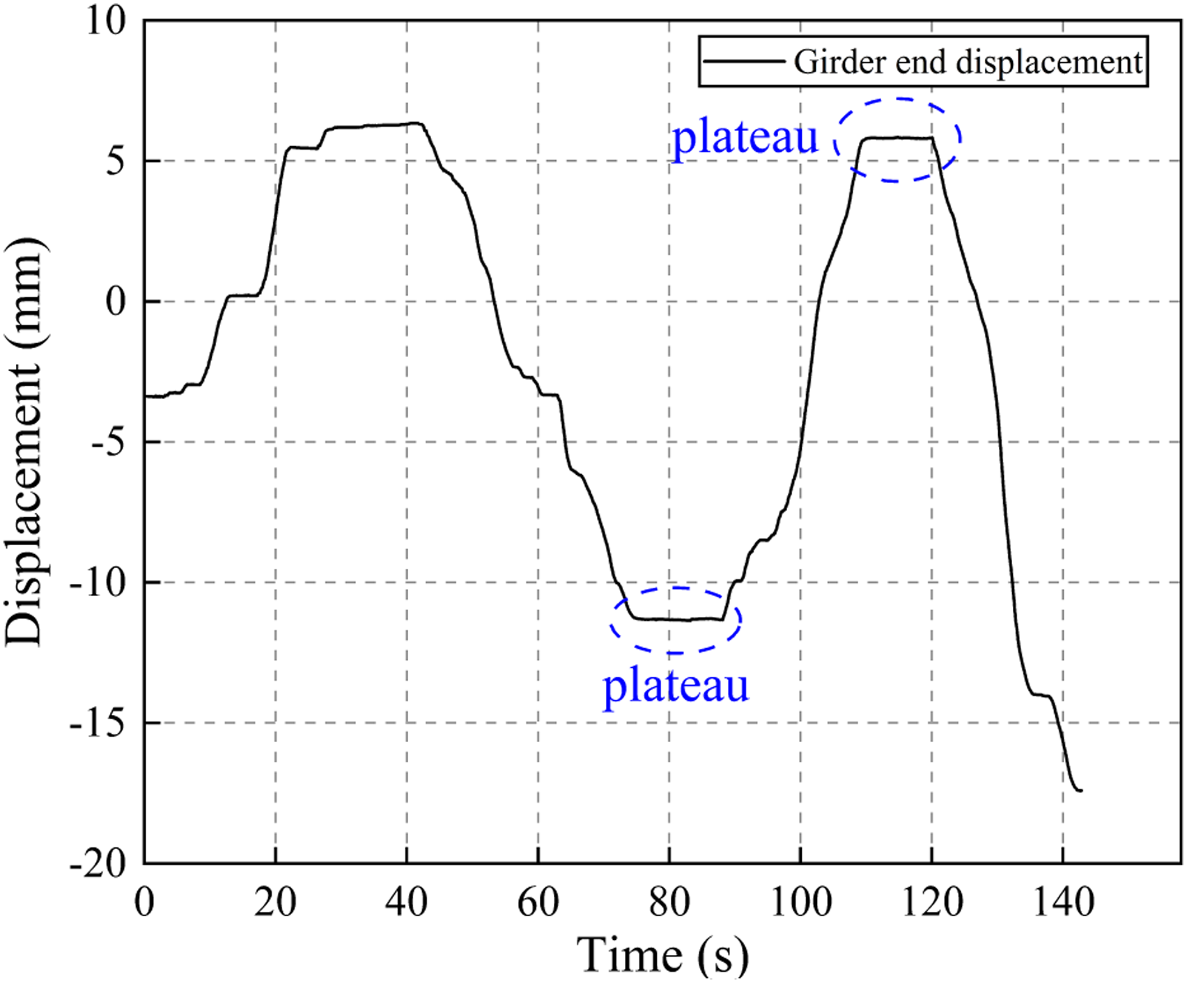

Unlike conventional finite element modeling approaches for bridge structures, this study adopts the CONTA178 element to model the vertical bearings. CONTA178 is a point-to-point contact element defined by two nodes. In the present model, these two nodes are selected from the corresponding locations on the transverse beam of the pylon and the main girder, representing the centers of the upper and lower bearing surfaces, respectively. The contact normal direction of the element is automatically determined based on the spatial coordinates of the two nodes, eliminating the need for explicit definition of the contact orientation. In addition to providing vertical support stiffness, this element is also capable of simulating frictional behavior at the bearing interface. After specifying the friction coefficient μ, the program automatically evaluates the contact state based on the ratio between tangential $F_{S}$ and normal contact forces $F_{N}$ . When the tangential force $F_{S} \geq μ F_{N}$ , the contact interface transitions into a sliding or separation state, indicating that the main girder overcomes static friction and initiates relative motion. The pressure parameters sustained by the vertical bearings are automatically calculated based on the combined effects of the structural self-weight and the applied live loads. The obtained bearing reactions can reasonably represent the actual structural force state, thereby providing a reliable basis for determining the frictional force of the girder end restraint devices. CONTA178 element enables the consideration of bearing friction without significantly increasing model complexity, while avoiding the high computational cost and convergence difficulties commonly associated with solid-element-based modeling approaches.

In practical structures, bearings, dampers, and expansion joints jointly form a coupled longitudinal restraint system, while their mechanical functions are clearly differentiated. Specifically, bearings provide contact constraints and friction-based energy dissipation (Coulomb friction), dampers contribute velocity-dependent energy dissipation, and expansion joints together with other longitudinal restraints are modeled using equivalent springs, which provide relatively large longitudinal stiffness to control the displacement amplitude at beam ends, with stiffness values reflecting the characteristics of structural constraints. In the present model, these components are implemented based on distinct working mechanisms (velocity-dependent, frictional, and stiffness-based) and activation conditions, thereby achieving functional separation and avoiding physical coupling and constraint redundancy caused by stiffness superposition.

On-site vehicle load sequence construction

The process for constructing the on-site vehicle load sequence is illustrated in Figure 9. Initially, the loading sequence is derived from the joint database. Assuming a constant speed for all vehicles, the spatiotemporal sequence of the vehicle fleet is determined. Subsequently, using the load distribution model, equivalent nodal loads are determined at each time step. To account for vehicle-bridge interaction, a dynamic impact factor is applied. Finally, dynamic nodal loads are formulated based on on-site monitored vehicle data.

Figure 9.

The procedure of on-site vehicle load sequence construction.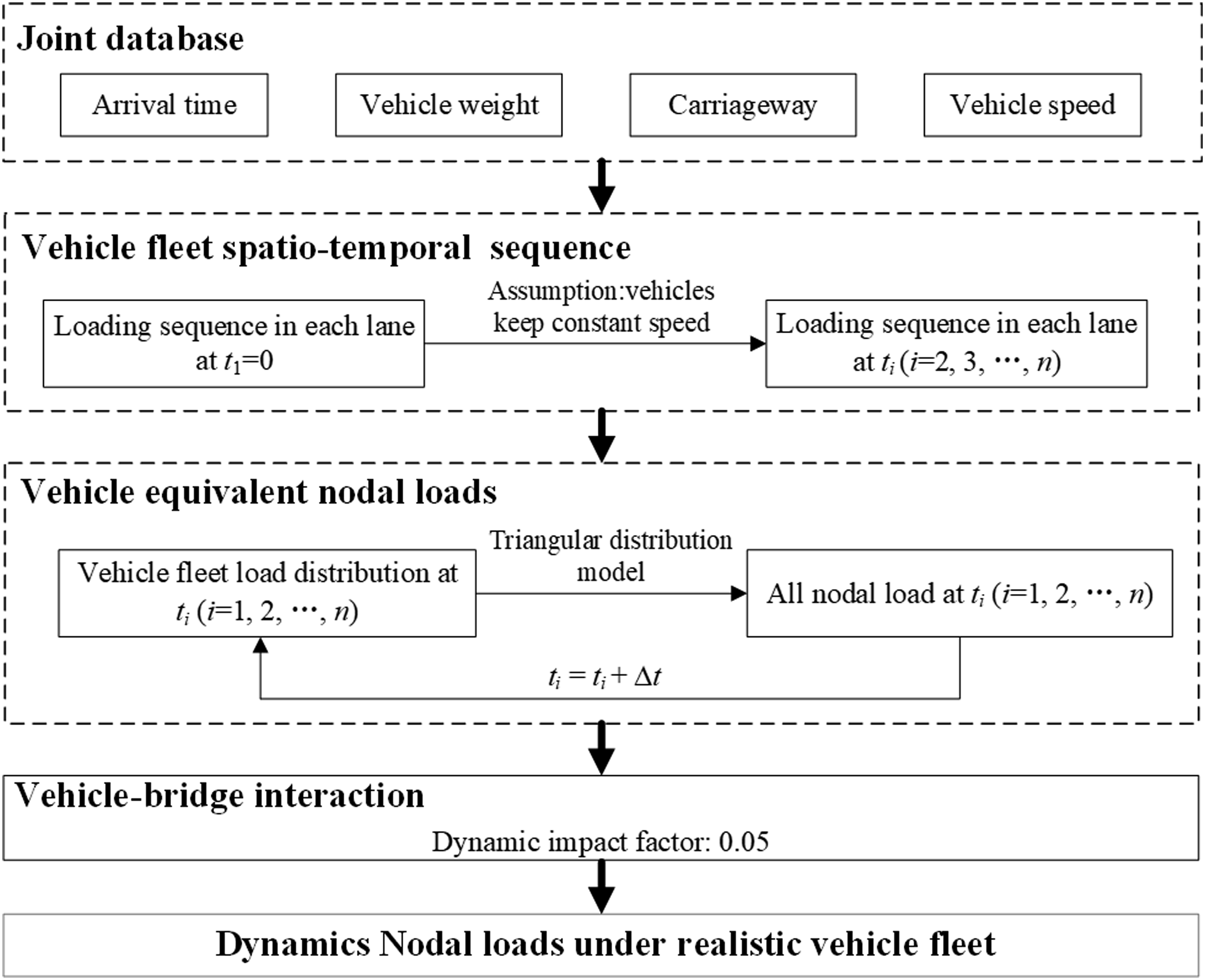

Vehicle fleet loading sequence

The database records the timestamps of vehicles entering the bridge, reaching the mid-span, and leaving the bridge. Based on the passing times at different monitoring sections and the corresponding segment lengths, the traveling speed of vehicles within each segment can be determined, thereby establishing a time–space mapping relationship for vehicle motion. Specifically, by taking the bridge entrance as the coordinate origin, the position of each vehicle relative to the origin at any given time can be calculated according to the starting time of the corresponding segment and the associated segmental speed, thereby enabling the construction of the actual vehicle load sequence. As illustrated in Figure 10, the arrival time of the first vehicle at the bridge entrance is set as t₁ = 0. The arrival time of the i^th vehicle is t_i. In this regard, the virtual distance of each vehicle from the bridge entrance is assumed as x_i = t_i × v_i, where v_i is the i^th vehicle speed.

Figure 10.

Simplified vehicle fleet load model.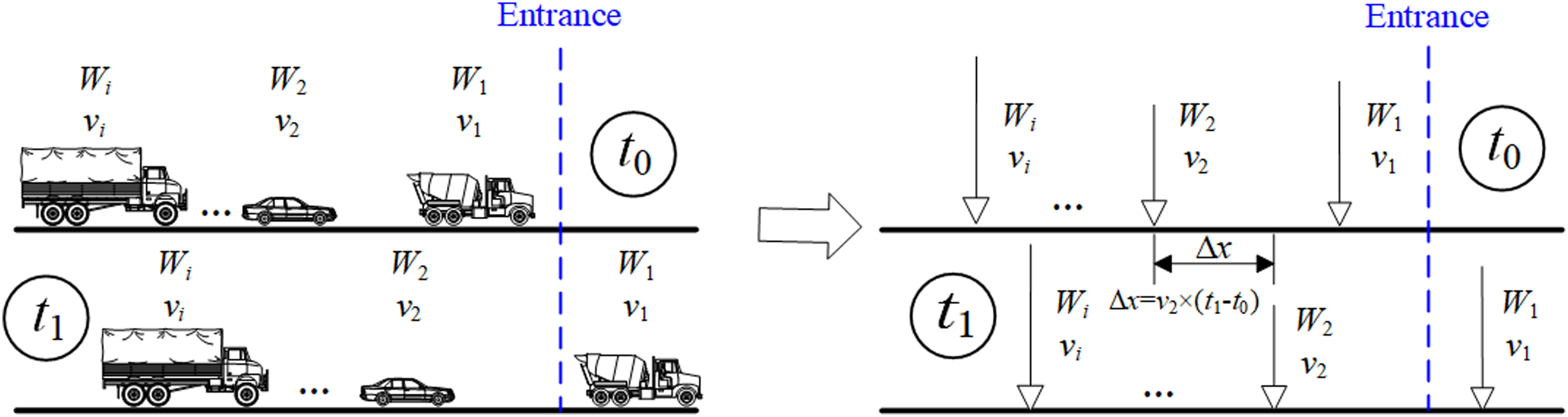

Due to the difficulty in accurately identifying the axle spacing of individual vehicles in actual traffic flow, the load of a single vehicle is simplified as a concentrated load with a magnitude equal to the total vehicle weight, applied at the geometric center of the vehicle. This concentrated load assumption is applicable to analyses focusing on the global structural response of bridges, particularly when the bridge span is relatively large compared with the vehicle axle spacing, such that the influence of axle load distribution on overall displacement and internal force responses is limited. Under this assumption, the vehicle convoy can be represented as a series of concentrated loads, as illustrated in Figure 10. The effects of vehicle–bridge interaction will be further discussed in subsequent sections.

Vehicle equivalent nodal loads

In finite element models, loads must be applied at nodes, necessitating the conversion of spatially continuous vehicle fleet loads into discrete nodal loads. This study introduces an equivalent method based on shape functions and the principle of virtual work to achieve this. Shape functions are interpolation functions used in the finite element method to describe the displacement field within an element. They establish the relationship between the displacement at any position inside the element and the nodal degrees of freedom. As shown in Figure 11(a), the red and blue curves represent the shape functions associated with the two nodes of a beam element, respectively. Taking the transverse degree of freedom of the beam element as an example, when the shape function at the left node equals 1, the value at the right node is 0, indicating that each node only directly governs its own displacement. Based on this, the displacement at any point within the element can be obtained by interpolating the nodal displacements using the shape functions. To ensure consistency and compatibility of the element interpolation, the shape functions satisfy $N_{1 (ξ_{1})} + N_{2 (ξ_{2})} = 1$ at any position within the element, which guarantees the conservation of load distribution and satisfies the principle of virtual work equivalence.

Figure 11.

Shape functions and equivalent load transformation process.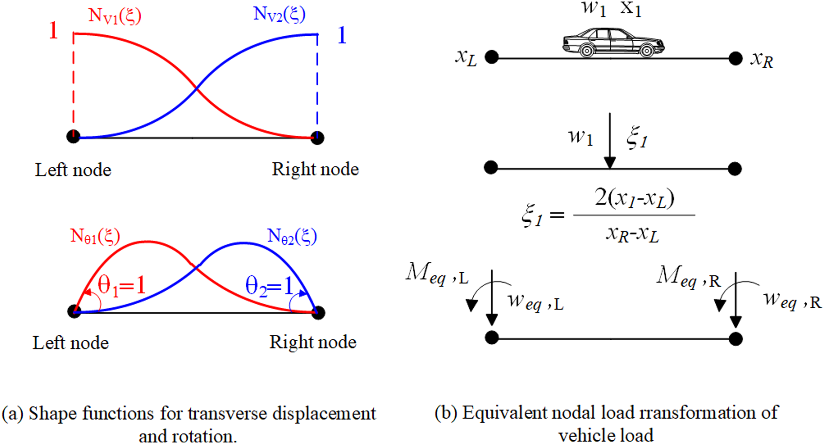

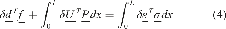
Considering the beam element configuration shown in Figure 12, and applying the principle of virtual work, the equilibrium equation is expressed as:

δ {\underline{d}}^{T} \underline{f} + \int_{0}^{L} δ {\underline{U}}^{T} \underline{P} d x = \int_{0}^{L} δ {\underline{ε}}^{T} \underline{σ} d x

(4)

where

δ

denotes the virtual variation operator.

d

and

f

represent the nodal displacement vector and nodal force vector, respectively.

U

is the displacement field while

P

denotes the distributed load. In addition,

ε

and

σ

correspond to the strain and stress fields, respectively.

Figure 12.

Degree of freedom and load distribution of the beam elements.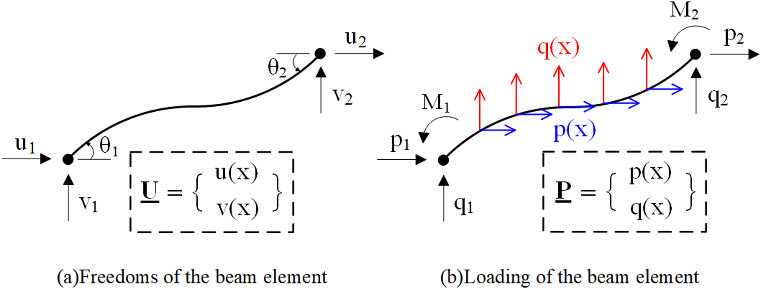

Based on the previously defined shape functions, the displacement at any point within the element domain can be expressed in terms of the shape functions and nodal displacements, that is, $δ \underline{U} = \underline{N} δ \underline{d}$ . By taking the transpose of both sides and substituting into the governing equation, the following expression can be obtained:

\int_{0}^{L} δ {\underline{U}}^{T} \underline{P} d x = δ {\underline{d}}^{T} \int_{0}^{L} {\underline{N}}^{T} \underline{P} d x

(5)

where N is the shape function matrix, which can be obtained from the ANSYS documentation according to the selected element type.

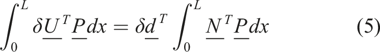
From equation (5), it can be observed that the work done by an arbitrarily distributed load over the element is equivalent to the work done by an equivalent nodal force with magnitude $\int_{0}^{L} {\underline{N}}^{T} \underline{P} d x$ acting at the nodes, that is,

F_{e q} = \int_{0}^{L} {\underline{N}}^{T} \underline{P} d x

(6)

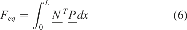
Considering the vehicle load as a concentrated force and normalizing the element length, the expression can be further simplified as

F_{e q} = \int_{0}^{L} {\underline{N}}^{T} \underline{P} d x = W_{i} N_{(x_{i})} = W_{i} N_{(ξ_{i})}

(7)

where W_i denotes the weight of the i-th vehicle (kN), and x_i indicates its position within the corresponding element. The natural coordinate ξ_i, normalized by the element length, lies within the interval [−1, 1].

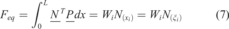
Figure 12, based on equation (7), illustrates the detailed procedure of converting vehicle loads into equivalent nodal forces. Considering the vehicle load as a vertical concentrated force, the equivalent load does not induce axial projection within the element. Therefore, Figure 11(a) focuses solely on the beam element’s transverse displacement and rotation shape functions. First, the element containing the vehicle is identified based on the vehicle’s position. The coordinates of the element’s two end nodes are then obtained, and the vehicle’s Cartesian coordinates are transformed into the element’s natural coordinate system. By substituting the natural coordinate into the corresponding shape functions and multiplying by the vehicle load, the equivalent nodal forces can be determined. The concentrated force within the element is eventually converted into equivalent vertical forces and bending moments applied at the beam element’s nodes. The final step is to assemble all vehicles into a representation of the actual on-site traffic fleet. In practical scenarios, multiple vehicles present simultaneously on the bridge deck. To address this, a linear superposition method is developed to handle multi-vehicle conditions. Based on the spatiotemporal sequence of the vehicle fleet, the positions of all vehicles at each timestamp are determined. Using the procedure described earlier, the equivalent nodal loads for each vehicle within its respective element are computed. Figure 13 illustrates the vertical equivalent forces induced by vehicle loads. At a specific time instant, the load applied to Node 2 can be quantified as $P = w_{1} N_{v_{2} (ξ_{1})} + w_{2} N_{v_{1} (ξ_{2})}$ . To obtain the time-varying load history at each node, equivalent loads are calculated at each time step throughout the simulation period. The nodes are then subjected to these time-dependent vertical forces and bending moments, thereby reproducing the dynamic loading effects of the on-site vehicle load sequence. This approach effectively transforms the on-site vehicle load sequence into a time history of equivalent nodal forces and moments.

Figure 13.

A superposition method of vehicle load.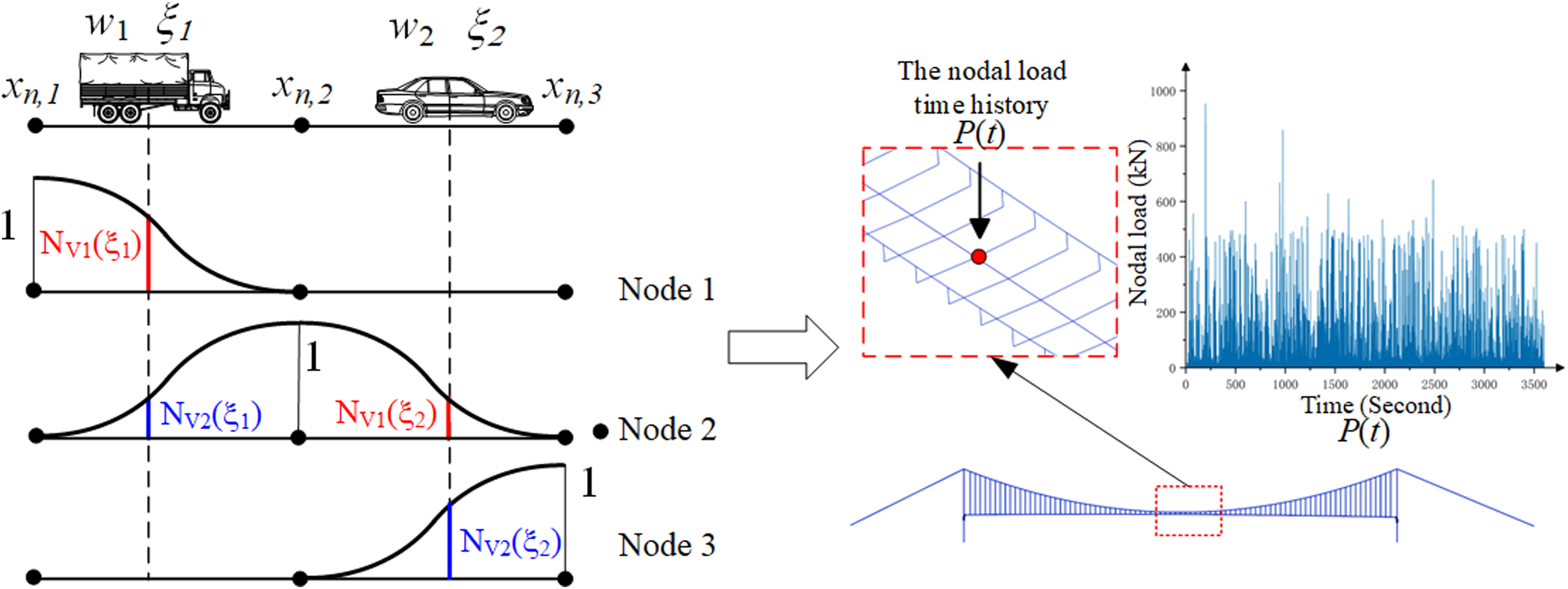

Considering that the main girder is modeled as a single beam element while the traffic loads are distributed across six lanes, the lane loads need to be transferred to the bridge centerline, that is, the axis of the beam element in the finite element model. Meanwhile, an additional bending moment induced by this transverse eccentricity must also be considered and applied to the model. This additional moment can likewise be treated as part of the time-history loading described above, together with the vertical forces, to more appropriately represent the overall effect of multi-lane stochastic traffic loads on the main girder.

Vehicle-bridge interaction

Since dynamic impacts of vehicles induced by vehicle-bridge coupling vibration will affect the structural response, it is of significance to accurately simulate the dynamic response. This study is conducted based on real traffic flow data. While vehicle–bridge coupled vibration analysis can improve modeling accuracy, it also significantly increases computational cost. For realistic traffic flow conditions, explicitly modeling the interaction for each vehicle would lead to extremely complex modeling procedures and prohibitively high computational demands, making it impractical for engineering applications. Therefore, a dynamic impact factor is adopted to account for the vehicle–bridge interaction effects in an equivalent manner. Based on previous studies, the dynamic impact factors of typical vehicle types are between 0.032 and 0.052 subjected to a very good road roughness case (Deng and Cai, 2010; Deng et al., 2018; Obrien et al., 2010; Shi et al., 2008; Wang et al., 1992). The studied bridge has a very good road roughness condition since it is under the highest construction and maintenance standard in China. In this regard, the dynamic impact factor is set as 0.05 according to the China bridge design code in this case study, which is discussed in detail in our paper (Xu et al., 2021).

Finite element model updating

A model updating method for the finite element models is developed based on on-site data by using GAs. The primary objective is to minimize the discrepancy between simulated and field measured girder end displacements. A combined ANSYS and MATLAB simulation is employed, integrating a GA to determine the optimal parameter values. The flowchart detailing this proposed finite element model updating method is presented in Figure 14.

Figure 14.

The flowchart of the finite element model updating method.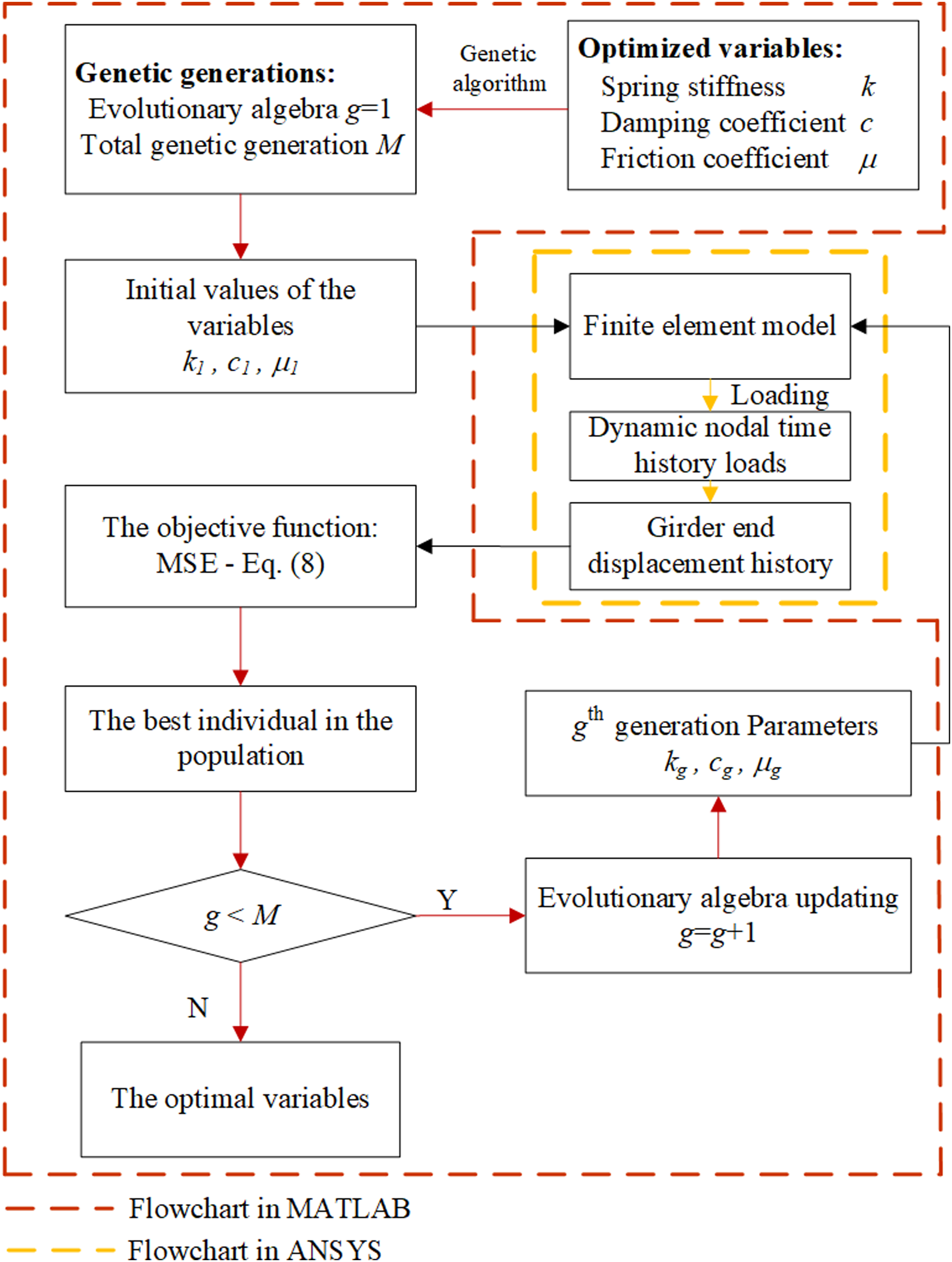

In the finite element model, variations in spring stiffness (k), damping coefficient (c), and friction coefficient (µ) significantly impact the girder end displacement. Thus, these parameters are selected as optimized variables. The reasonable range of these parameters can be determined through finite element trial analyses. Specifically, an initial range of stiffness values is assumed, while other parameters are temporarily fixed. Based on previously obtained traffic load inputs, numerical simulations are performed, and the measured girder end displacement response is used as a reference. The admissible stiffness range is then adjusted such that the measured response lies within the envelope of the simulated displacement responses. This procedure ensures that the selected bounds are physically consistent and capable of covering the observed structural behavior.

A similar strategy is adopted for other parameters. For the friction coefficient, an upper bound is defined such that the corresponding simulated plateau duration is not smaller than that observed in the measurements (noting that the plateau duration approaches zero in the absence of friction). For the damping coefficient, a value of zero corresponds to a purely elastic boundary condition (assuming a friction coefficient of zero), in which the linear spring provides restoring force without any energy dissipation, resulting in noticeable local oscillations in the girder end displacement response. The upper bound of the damping coefficient is defined such that it can effectively suppress the aforementioned local oscillations in the displacement response.

The GA is employed to determine the optimal values of the model variables. Inspired by the principles of natural selection, the genetic algorithm (GA) is a widely used evolutionary optimization technique in engineering applications. It operates by iteratively evolving a population of candidate solutions toward an optimal or near-optimal solution through biologically inspired operations such as selection, crossover, and mutation. This process enables efficient exploration of the solution space and progressive improvement of solution fitness across generations.

In the present study, GA is adopted due to its strong global search capability, robustness, and independence from gradient information or strict assumptions on the objective function. These characteristics make it particularly suitable for the complex, nonlinear, and multi-parameter coupled finite element model updating problem with multiple constraints considered herein. Prior studies have also demonstrated that GA is effective in solving high-dimensional engineering optimization problems, further supporting its application in this work. The variable ranges for the GA and other relevant settings are provided in Table 1. Initially, the optimization parameters are randomly assigned values within their specified ranges and input into the ANSYS model. Next, using the predefined equivalent nodal load, a joint simulation of the on-site vehicle load sequence is conducted in ANSYS, producing girder end displacement curves for the simulated period. These simulated displacement curves are then compared with the field measurements from the short-term monitoring system.

Table 1.

Genetic algorithm parameter settings.

Optimization variables	Value range	Algorithm parameters	Values
Stiffness (kN/m)	[6400, 32,000]	Popsize	50
Damping coefficient (N · S · m⁻¹)	[200,000, 800,000]	Crossover probability	0.4
Friction coefficient	[0, 0.2]	Mutation probability	0.001
		Evolutionary generations	50

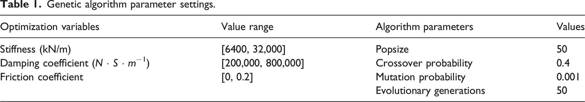
The parameters of the genetic algorithm (GA), including population size, crossover rate, and mutation rate, are determined based on ranges recommended in the literature and engineering practice to ensure algorithm convergence and stability. Generally, the crossover rate is set within 0.4–0.9, the mutation rate within 0.001–0.1, and the population size is related to the number of optimization variables: approximately 50 when the number of variables is less than 5, and about 200 when the number is greater than 5.

Within these reasonable parameter ranges, the influence of GA parameters on the final optimized results is relatively limited, and they mainly affect the convergence efficiency and the stability of the search process. An independent validation dataset is further introduced to evaluate the updated model. The results demonstrate that the model still achieves good predictive accuracy on data not involved in the optimization process, thereby confirming the reliability of both the parameter settings and the optimization results.

The objective function between the simulated and observed values is evaluated using the mean squared error (MSE) index, defined as: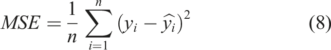

M S E = \frac{1}{n} \sum_{i = 1}^{n} {(y_{i} - \hat{y_{i}})}^{2}

(8)

where

y_{i}

represents the simulated girder end displacement,

\hat{y_{i}}

denotes the measured values obtained from the short-term monitoring system.

In this study, MSE serves as the objective function within the GA. During each iteration, the optimal variables from the current population are recorded and evolved into the next generation, generating new optimized variables. This process is repeated until the final optimization is achieved.

Results and discussions

Convergence of the GA

Figure 15 shows the convergence process of the GA in terms of MSE over a series of generations. The vertical axis represents the MSE, which quantifies the difference between the computed structural response and the target reference data. The horizontal axis corresponds to the generation index, indicating the evolutionary progression of the population during optimization.

Figure 15.

Result for MSE-based convergence of the Genetic Algorithm.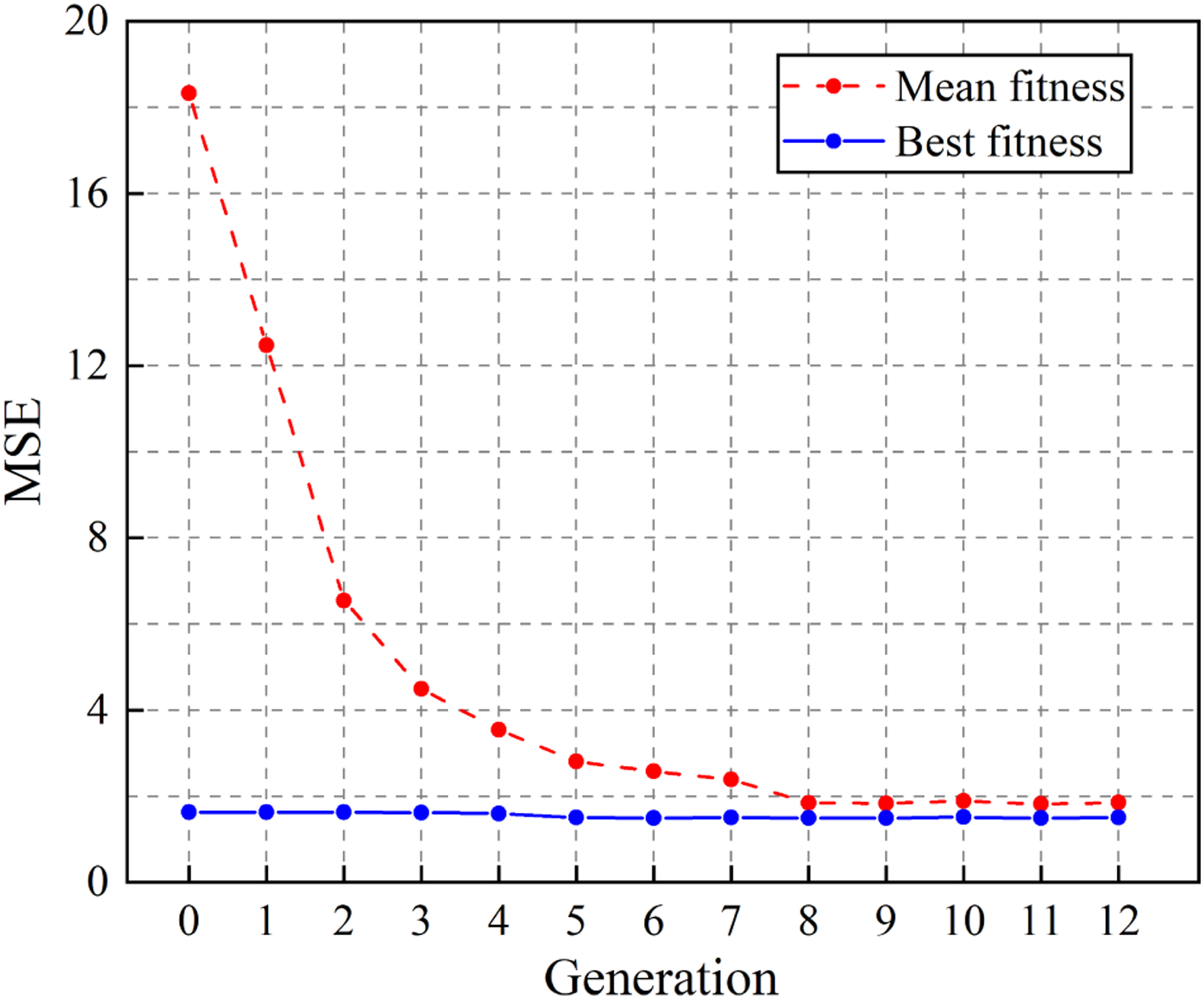

Two sets of data are presented in Figure 15: the blue markers represent the best individual (i.e., the lowest MSE) in each generation, while the black markers denote the average MSE across the population. At the initial stage (Generation 0), the population exhibits considerable variability in performance, as indicated by the large gap between the best and mean MSE values. The mean fitness is 18.7365, reflecting the poor quality of the randomly initialized individuals, while the best fitness value is already relatively low (1.61374), suggesting that some initial solutions lie near the optimal region of the search space.

As generations progress, mean fitness values show a rapid decrease, especially within the first five generations. This indicates that the algorithm is effective in quickly eliminating low-quality individuals and guiding the population to better-performing regions. The convergence trend continues over the next few generations, but with a diminishing rate of improvement. After Generation 8, the fitness values begin to plateau, and both curves show signs of stabilization. In the final generation, the algorithm had achieved a best MSE of 1.53627 and a mean MSE of 1.8753. The narrow gap between these two values indicates that the global minimum was approaching, but also that the overall population exhibited strong consistency. This convergence behavior confirms that the GA is capable of reliably identifying near-optimal parameters for the structural system under consideration.

Although the maximum generation count was set to 50 in the initial configuration, the algorithm was terminated early at Generation 12. This decision was based on the observation that the MSE values no longer improved significantly beyond this point. In fact, minor oscillations in both the best and mean fitness curves suggest that the population had already converged and that further iterations would likely yield negligible gains. In this regard, early stopping was applied to reduce unnecessary computation while preserving the quality of the solution.

Overall, the convergence behavior indicates that the GA is effective in minimizing the MSE, and is well-suited for parameter identification tasks involving non-linear systems with complex response characteristics. The three parameters optimized by the GA, spring stiffness, damping coefficient, and frictional coefficient, converged to optimal values of 14,563.5 kN/m, 654,371 $N \cdot S \cdot m^{- 1}$ and 0.0330,256, respectively. These identified parameters will be used in the subsequent analysis.

Validation of the finite element model

Based on the final set of parameters obtained through the GA optimization presented earlier, the displacement response at the girder end under on-site traffic fleet was simulated using the proposed finite element model. Figure 16 illustrates a comparison between the measured displacement (black line) obtained from the sensors and the simulated response (red line). The results demonstrate a high level of consistency between the two datasets, indicating the model’s capability to replicate the essential dynamic behavior of the structure under real traffic conditions.

Figure 16.

Comparison of measured and FE simulated girder end displacements.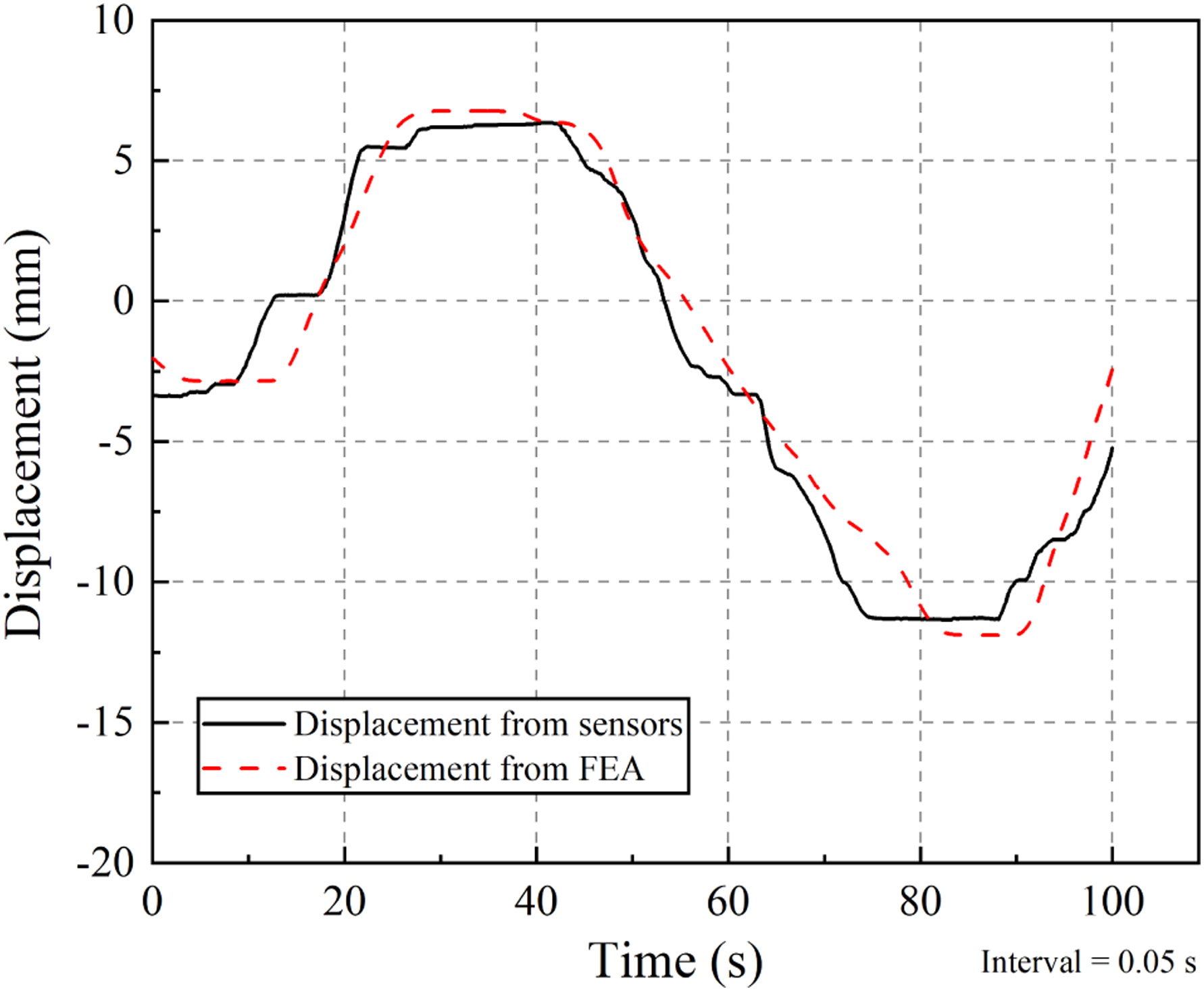

To begin with, the Pearson correlation coefficient between the measured and simulated displacement curves is 0.9832, suggesting a strong consistency in their global trends over the entire observation period. The measured response reaches positive peaks at approximately 30 s, and a negative peak near 85 s. The finite element simulation successfully captures these key response phases with minimal time lag, confirming the effectiveness of the model in reproducing the structure’s real-time behavior under complex loading scenarios. Minor deviations observed between 65 and 95 s may stem from simplifications in the traffic input model, where vehicles were assumed to move at constant speed without considering acceleration or braking behavior. In addition, potential time-synchronization errors between the field camera recordings and simulated vehicle positions may contribute to small discrepancies in the displacement profiles. During this time period, the cumulative displacement measured by the sensor was 35.93,489 mm, while the finite element simulation result was 38.57,127 mm, showing very close agreement.

Secondly, the simulated displacement magnitudes exhibit strong agreement with the measured peak values. Sensor data recorded maximum displacements of approximately 6.2 mm and −11.5 mm, while the finite element model produced corresponding values of 6.7 mm and −11.9 mm. The maximum relative error across these peaks is less than 10%, which is acceptable in the context of field-validated structural analysis. These results suggest that the optimized stiffness and damping parameters, including the calibrated spring and dashpot elements, are effective in capturing both the amplitude and timing of structural responses under transient vehicular loads.

Third, a key non-linear behavior, the plateau observed during changes in displacement direction, was accurately reproduced. Specifically, in the intervals from 77 to 90 seconds, the girder displacement remains nearly constant, suggesting a temporary static equilibrium due to friction at the supports. This phenomenon is physically interpreted as the girder overcoming static friction before resuming movement. The finite element model captures this response through the non-linear spring-damper element COMBIN37 and the 3D point-to-point contact element CONTA178.

Overall, the close correspondence between the measured and simulated displacements across trend, magnitude, and non-linear behavior strongly validates the proposed FE model. The combination of accuracy, efficiency, and physical realism highlights its suitability for practical engineering applications involving dynamic vehicle-structure interaction.

To ensure the validity of the finite element model parameter calibration, an additional independent set of real vehicle load sequences was used for verification. As shown in the Figure 17, the simulated results are in good agreement with the measured responses in both magnitude and overall trend. First, the numerical simulation captures the overall response behavior observed in the measurements. Second, the plateau stage associated with changes in the direction of girder motion is successfully reproduced, with a comparable duration. Finally, the measured cumulative girder end displacement is 34.75,099 mm, while the simulated result is 33.89,293 mm, yielding a small error of only 2.5%.

Figure 17.

Comparison of measured and FE simulated girder end displacements.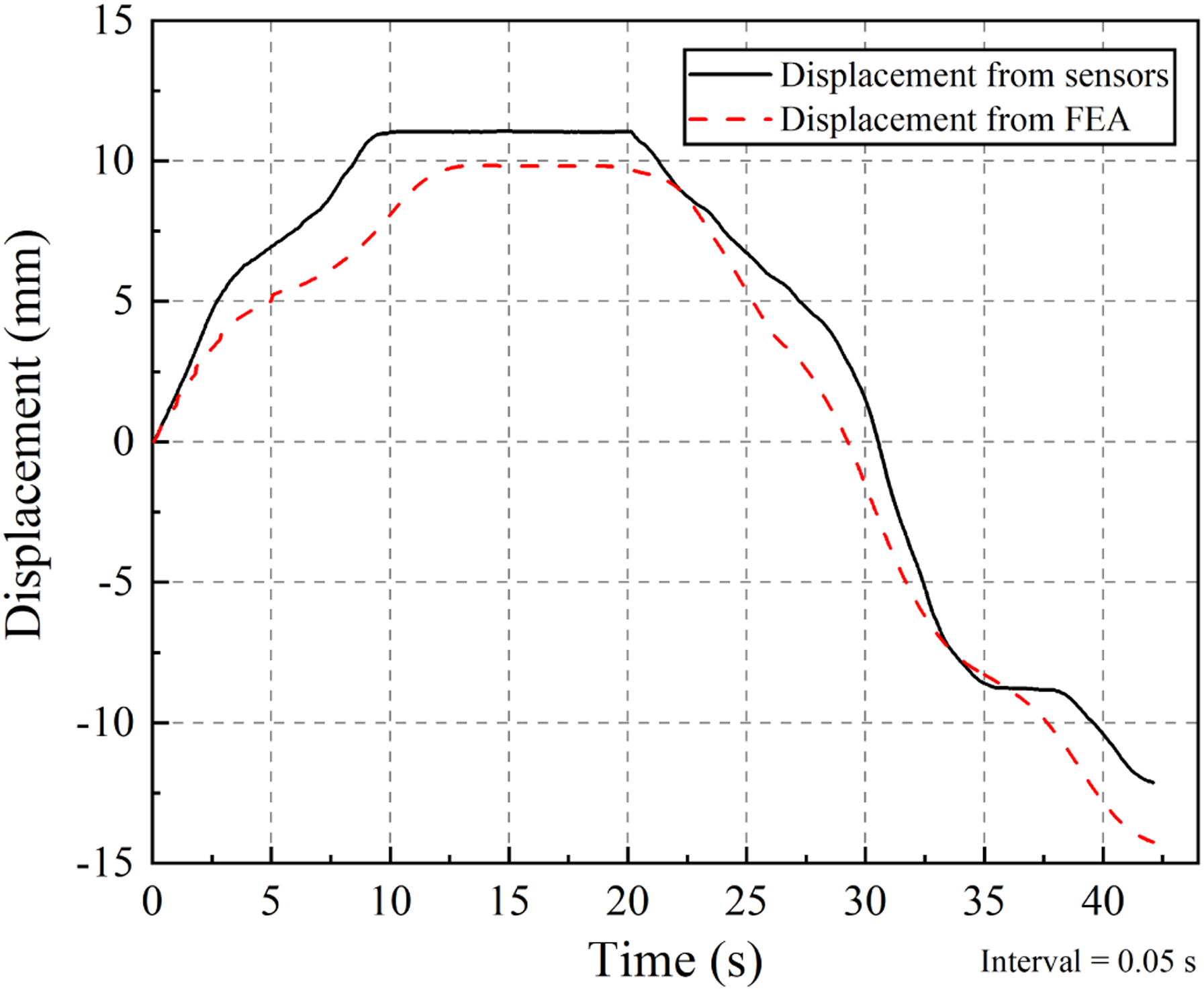

Key parameter discussions

Vehicle load effects are critical indicators of a bridge’s structural safety and long-term durability. In the absence of accurate data on actual traffic conditions, conventional design often relies on standardized live load models, as prescribed by design codes, with appropriate adjustment factors. Significant discrepancies may arise for long-span suspension bridges, where the design live loads may not accurately reflect the actual operational loading experienced during service. These deviations can lead to either over-conservative or under-conservative maintenance strategies, ultimately affecting the bridge’s lifecycle cost efficiency and practical applicability in operation and management.

To more accurately capture the bridge’s dynamic response under vehicle loads, this study first utilizes a finite element model that has been calibrated based on actual vehicle loading sequences, as previously discussed. By incorporating measured traffic data into the model, the resulting simulation offers a more realistic representation of the structural behavior under real-world loading conditions, compared to models relying solely on idealized or code-based load assumptions. Building upon this calibrated framework, stochastic traffic simulations are then introduced to represent possible future traffic patterns.

Compared with the vehicle load sequences constructed based on field-measured data in the previous section, the stochastic traffic model can better capture more complex traffic behaviors, including vehicle acceleration and deceleration, overtaking, and lane-changing processes. Specifically, based on vehicle information obtained from the bridge monitoring system, different vehicle types are first classified. Subsequently, the probability density functions of vehicle speed and vehicle weight are obtained by fitting mixed normal distributions and mixed lognormal distributions, respectively.

On this basis, according to the statistical distributions of the measured vehicle parameters, the Monte Carlo method is adopted to randomly sample key variables such as vehicle type, weight, and speed, thereby generating stochastic vehicle load sequences under a given traffic volume. The overall procedure for generating stochastic vehicle loads is similar to that of the actual traffic load sequences. The main difference lies in that vehicle speed and weight are randomly generated based on statistical distributions, while additional acceleration–deceleration behavior criteria and car-following models are introduced in the traffic speed simulation to improve realism. Random traffic flow modeling, including vehicle type classification, acceleration–deceleration behavior, and car-following models, can be implemented following the approaches reported in the relevant literature (Xu et al., 2010).

In this study, vehicle weight and speed are treated as key variables to capture the dynamic response of the bridge under stochastic traffic flow. Each simulation represents a one-hour traffic scenario. For stochastic traffic flow simulations, the vehicle traveling distance within a single time step should not be excessively large, so as to ensure the continuity of the moving load process and the accuracy of the structural dynamic response simulation. A time-interval sensitivity analysis can be conducted to determine an appropriate time interval. For the same stochastic traffic flow scenario, simulations can be performed using different time intervals, and the corresponding girder end displacement time-history curves can be obtained. When the discrepancies among the displacement time-history curves corresponding to different time intervals remain within an acceptable error range, the selected time interval can be considered adequate for the analysis and may be adopted as the recommended value. In the subsequent stochastic traffic flow simulations, a time interval of 0.1 s is adopted. Under this configuration (Intel® Core™ i7-11800H processor, 8 cores and 16 threads, with 32 GB of RAM), the simulation of 1 h of stochastic traffic flow data required approximately 6 h of computational time.

Girder end displacement under varying traffic flow levels

The simulation results of girder end displacement and its relative frequency distribution for the Huangpu Bridge under different one-way traffic volumes of 1500, 2000, and 2500 vehicles per hour (assuming identical traffic volumes in the opposite direction) are shown in Figure 18. The bridge considered in this study is a highway bridge. Based on observed traffic conditions, when the traffic volume is approximately 2200 vehicles/hour, the traffic flow generally remains in a free-flow state without entering typical congestion. Therefore, the upper bound of 2500 vehicles/hour adopted in the stochastic traffic simulations still corresponds to normal driving conditions rather than a fully congested regime.

Figure 18.

Girder end displacement simulations (left) and corresponding relative frequency histograms (right) under different traffic flow levels.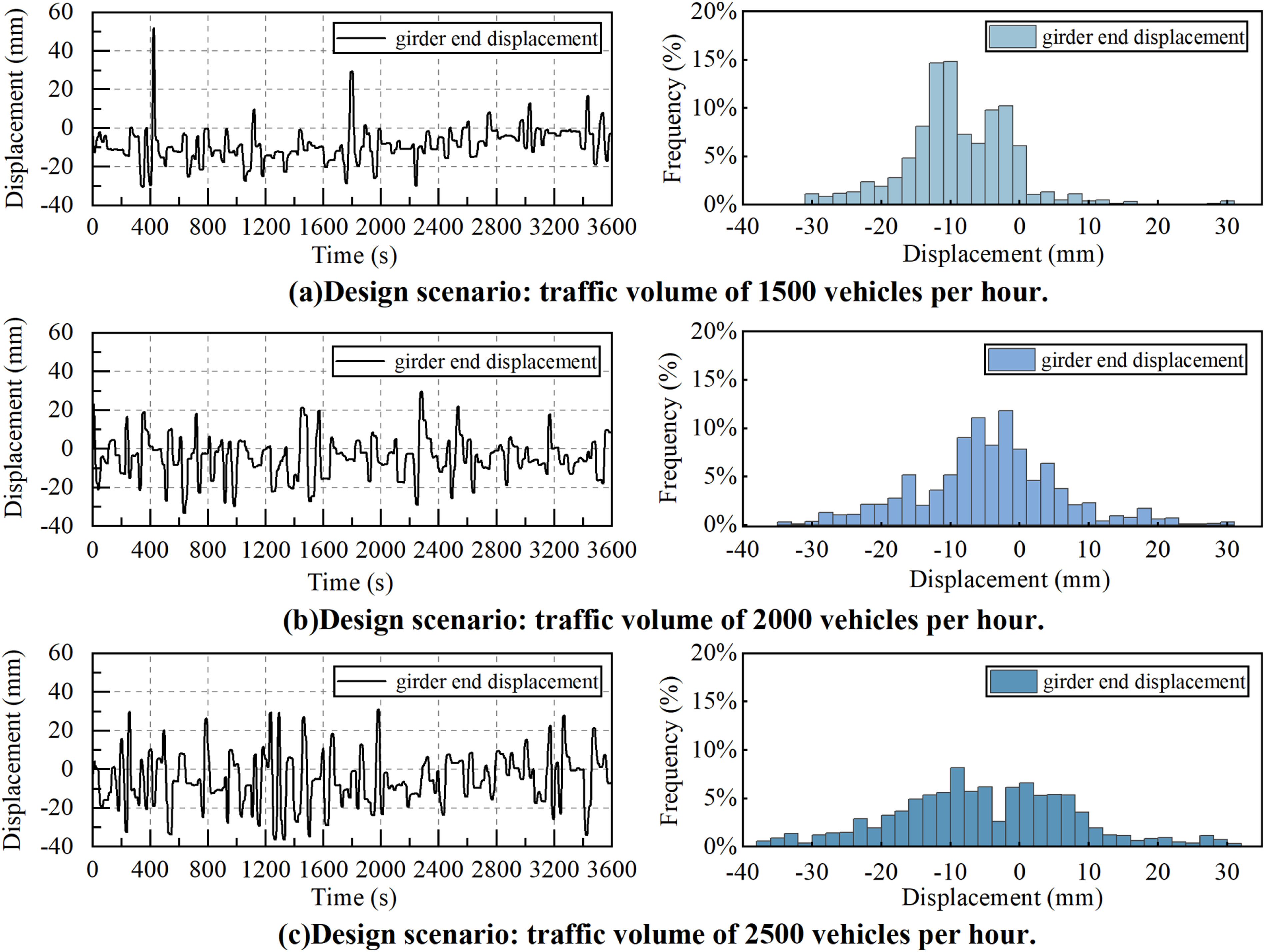

When the traffic flow is 1500 vehicles per hour, displacements are primarily concentrated within the range of −15 mm to 5 mm, showing a relatively narrow and peaked distribution. However, as the flow increases to 2000 and 2500 vehicles per hour, the displacement range expands significantly—from approximately −30 mm to 10 mm up to nearly −40 mm to 30 mm. With increasing traffic volume, the frequency histogram of girder end displacement shows a clear outward spreading trend on both sides, indicating that the probability of large-amplitude displacements increases significantly.

Girder end displacement under varying heavy vehicle ratios

To investigate the influence of heavy vehicle proportion on girder end displacement, a series of simulations were conducted by varying the percentage of heavy vehicles in random traffic flows. The one-way traffic volume was fixed at 1500 vehicles per hour, while the heavy vehicle ratio was set at five levels (Level 1 to Level 5). Level 1 represents a baseline scenario with a typical traffic composition, where the proportion of heavy vehicles is approximately 21%. This ratio was then increased to 30% (level 2), 35% (level 3), 40% (level 4) and 45% (level 5), respectively. The finite element simulation results corresponding to each scenario are illustrated in Figure 19.

Figure 19.

Girder end displacement simulations (left) and corresponding relative frequency histograms (right) under different heavy vehicle proportions.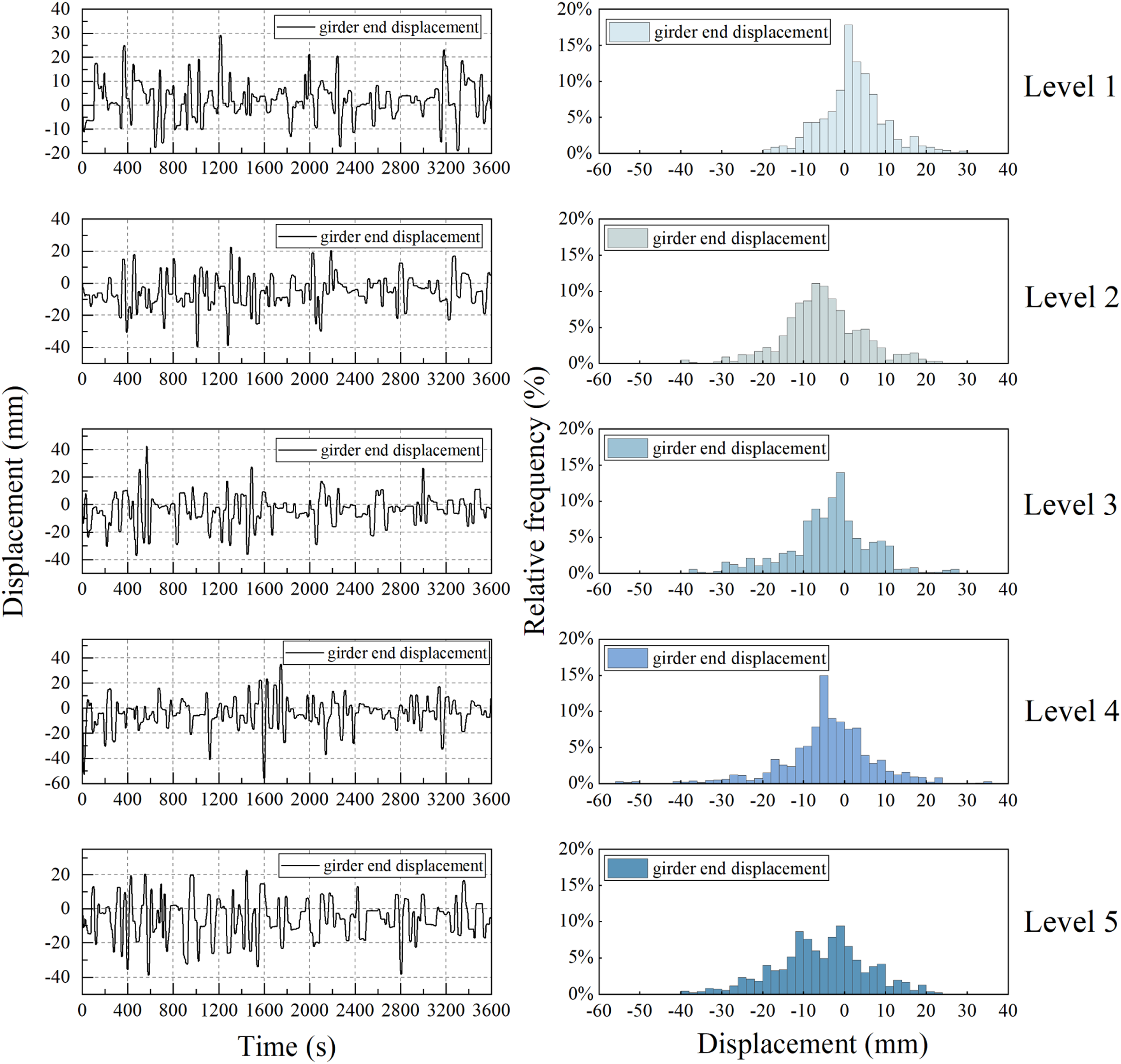

The frequency distribution of girder end displacements indicates that as the proportion of heavy vehicles increases, the magnitude of girder end displacements becomes significantly larger, and the overall distribution tends to flatten. Under Level 1 conditions, displacements are primarily concentrated within the range of −10 mm to 10 mm. However, with increasing heavy vehicle ratios, the histogram visibly broadens. By Level 5, the primary displacement range has expanded considerably, spanning from approximately −40 mm to 20 mm.

Girder end cumulative displacement discussion

Figure 20 illustrates the relationship between traffic volume and cumulative girder end displacement. When the one-way traffic volume is 1500 vehicles per hour, the corresponding cumulative displacement is approximately 1357.032 mm. As the traffic volume increases to 2000 vehicles per hour, the displacement rises to 1764.758 mm, representing an increase of 407.726 mm, equivalent to approximately 30%. When the traffic volume reaches 2500 vehicles per hour, the cumulative displacement further increases to 2520.074 mm, which is about 1.9 times greater than that observed under the 1500 vehicles per hour condition.

Figure 20.

Girder end cumulative displacement at various traffic flow levels.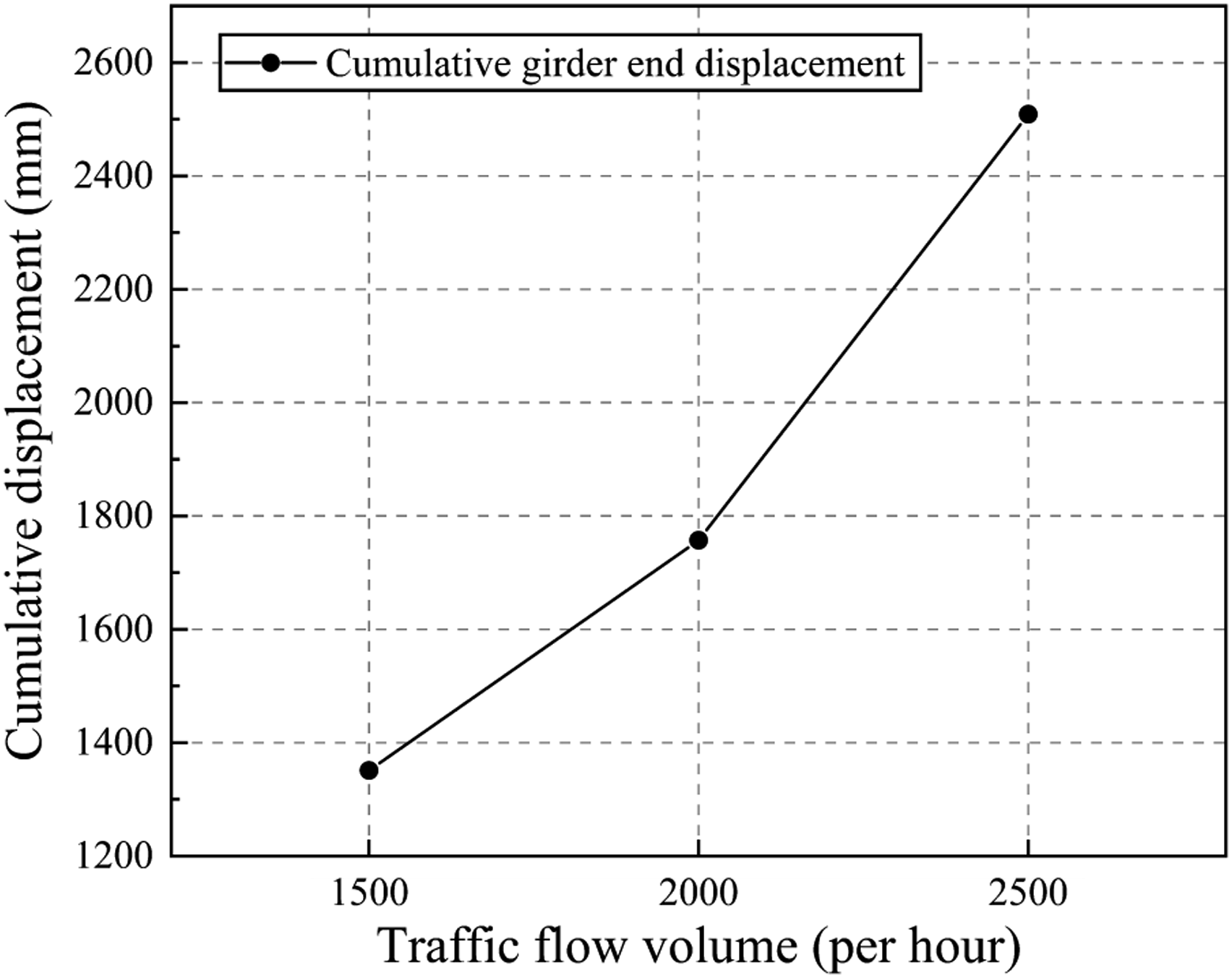

As shown in Figure 21, when the proportion of heavy vehicles was set to Level 1, the cumulative girder end displacement reached 1327.84 mm. As the heavy vehicle ratio increased to 30% (Level 2), the cumulative displacement rose to 1845.62 mm, representing an increase of approximately 1.4 times. Further increases in the heavy vehicle ratio to Level 3 and Level 4 resulted in continued growth in cumulative displacement, reaching 1960.803 mm and 213.437 mm, respectively. However, when the heavy vehicle proportion approached 40%, additional increases in the ratio did not lead to a significant rise in cumulative displacement.

Figure 21.

Girder end cumulative displacement at various heavy vehicle proportions.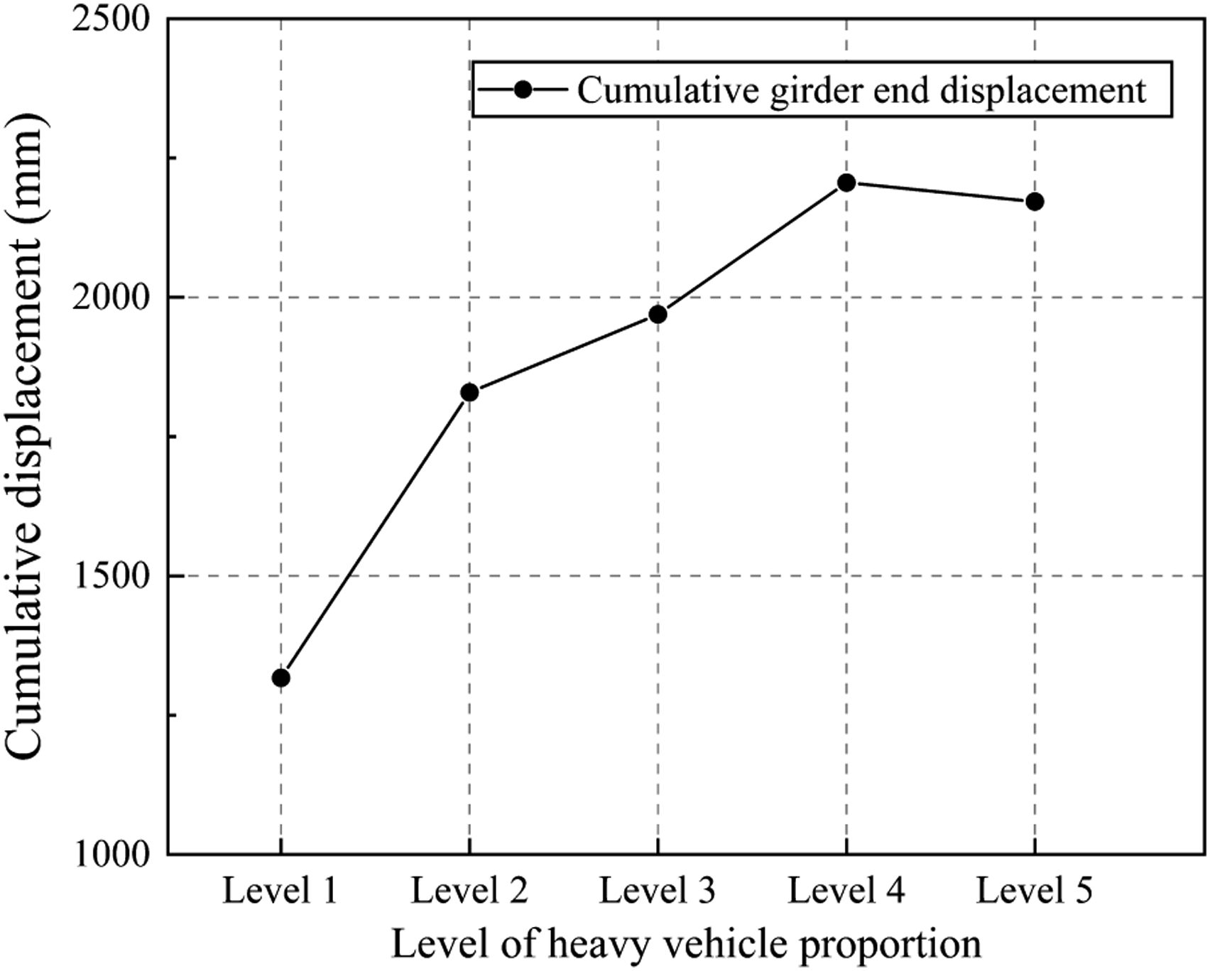

Overall, as both traffic volume and heavy vehicle proportion increase, the cumulative displacement at the girder ends increases significantly. For traffic volume, under non-congested conditions, the increase in traffic flow leads to a pronounced growth in cumulative girder end displacement. For different heavy vehicle ratio scenarios, the most significant increase in cumulative displacement occurs in the initial stage (from level 1 to level 2). However, when the heavy vehicle proportion approaches level 4, further increases in this ratio do not result in a noticeable rise in cumulative displacement. This phenomenon may be attributed to the relatively lower speeds of heavy vehicles. As the proportion of heavy vehicles increases substantially, the overall traffic flow speed decreases accordingly, thereby extending the action duration of girder end displacements. As a result, the accumulation effect gradually tends to stabilize rather than continue increasing significantly. It should be noted that such a dramatic increase in heavy vehicle ratio is unlikely to occur under realistic traffic conditions. In actual scenarios, a moderate increase in heavy vehicle proportion is expected to lead to greater cumulative displacements at the girder ends, which may accelerate bearing wear and compromise long-term structural performance.

It is worth noting that, based on the finite element analysis results, the high-amplitude responses of the beam-end displacement are primarily dominated by heavy vehicles. The results in Figure 17(a) further support this conclusion: under this loading condition, the peak girder end displacement reaches approximately 50 mm, indicating the passage of an overloaded vehicle. When a heavy truck imposes a load significantly larger than that of surrounding vehicles, the dynamic response of the main girder is often governed by this single vehicle. Relevant studies have also shown that heavy vehicles, due to their large mass and discrete spatial distribution, are more likely to induce an asymmetric stress state in the main girder, thereby significantly amplifying the longitudinal vibration response at the beam end (Gu et al., 2026).

For bridge maintenance purposes, the deck monitoring system should place particular emphasis on traffic volume as well as the weight and proportion of heavy vehicles. Simulation results indicate that increases in traffic flow and heavy vehicle ratio both lead to a nonlinear growth in cumulative girder end displacements. Such accumulation may accelerate fatigue damage development, promote bearing deterioration, and increase the demand on expansion joints and support systems. Prolonged exposure to high traffic loads can result in progressive degradation of critical components, thereby shortening the service life of the bridge and increasing future maintenance and repair requirements. In addition, overloaded vehicles should be given special attention, as their excessive loads can induce significant girder end displacements, potentially leading to damage of expansion joint restraint devices, such as loss or failure of bearing anchor bolts.

The finite element model developed in this study can be applied to the performance evaluation of bridges under future operational conditions. In addition to the aforementioned design scenarios involving different traffic volumes and heavy vehicle ratios, it can also be adapted to simulate other practical conditions as needed. For example, the friction coefficient can be modified to reflect bearing deterioration, and the velocity exponent of dampers can be adjusted to represent issues such as damper oil leakage.

Conclusions

This study proposes a finite element modeling approach refined using on-site vehicle load sequences, aiming to better capture the dynamic longitudinal motion behavior of long-span bridges under real-world traffic conditions. The model is designed to account for key nonlinearities, such as damping and friction effects. The major contributions of this work are summarized as follows:

(1) A practical nonlinear finite element analysis model considering multiple longitudinal restraints was developed. Viscous dampers were simulated using COMBIN37 elements, while the frictional interaction between the bearings and the stiffening girder was represented using CONTA178 contact elements. In addition, based on data from the bridge health monitoring system, actual traffic loads were transformed into equivalent nodal time-history loads using the principle of virtual work and applied to the model for transient dynamic analysis to simulate girder end displacement responses. This modelling strategy strikes a balance between computational efficiency and physical accuracy, achieving good agreement with observed displacement trends.

(2) The three key parameters governing longitudinal resistance are identified and calibrated using GA based on on-site vehicle load sequences. The GA proved effective in tuning the model to replicate real-world behaviour, significantly improving both convergence and predictive accuracy. By using the optimal parameters, the best MSE decreases to 1.50485, where the spring stiffness, damping coefficient, and frictional coefficient are 14,563.5 kN/m, 654,371 $N \cdot S \cdot m^{- 1}$ and 0.0330,256, respectively.

(3) Using a refined model, the longitudinal motion characteristics were analyzed under different traffic volumes and heavy-vehicle ratios. The results show that as both traffic volume and heavy-vehicle proportion increase, the accumulated displacement at the girder ends exhibits a nonlinear growth trend. Among the influencing factors, heavy-vehicle loads have a significant impact on the magnitude of girder end displacement.

In addition, the finite element model-updated with real-world traffic load inputs—offers a reliable and efficient tool for analyzing bridge dynamics under actual operational conditions. It incorporates key nonlinear behaviors and translates complex vehicle–structure interactions into realistic response predictions. Beyond estimating girder end displacements, the model is capable of outputting other critical response parameters, such as hanger stress histories and frictional force evolution, making it well-suited for long-term structural health monitoring and operational performance assessments of large-scale bridge systems.

Footnotes

ORCID iDs

Xiang Xu

Jiasheng Lan

Funding

The authors disclosed receipt of the following financial support for the research, authorship, and/or publication of this article: This work was supported by the National Key Research and Development Program of China (Grant No. 2022YFB3706704) and the National Natural Science Foundation of China (Grant No. 52308150). It was also supported by the Science and Technology Development Projects of China Railway Design Corporation Ltd. (Grant Nos. 2023A0248001, 2025A0248006, and 2025A0123801). The authors further acknowledge the support provided by the Big Data Computing Center of Southeast University.

Declaration of conflicting interests

The authors declared no potential conflicts of interest with respect to the research, authorship, and/or publication of this article.

Data Availability Statement

Some or all data, models, or code that support the findings of this study are available from the corresponding author upon reasonable request.*

References

Brownjohn

Koo

Scullion

, et al. (2020) Operational deformations in long-span bridges. In: Design, Assessment, Monitoring and Maintenance of Bridges and Infrastructure Networks. Routledge, pp. 144–162.

Deng

Cai

(2010) Development of dynamic impact factor for performance evaluation of existing multi-girder concrete bridges. Engineering Structures 32(1): 21–31. https://doi.org/10.1016/j.engstruct.2009.08.013

Deng

Duan

, et al. (2018) Study on vehicle model for vehicle-bridge coupling vibration of highway bridges in China. China Journal of Highway and Transport 31(7): 93–100.

Dong

Pan

Wang

, et al. (2024) Transformer‐enhanced traffic load simulation for wear evaluation of bridge expansion joint. Structural Control and Health Monitoring 2024(1): 6631877. https://doi.org/10.1155/2024/6631877

Feng

Zhang

Jing

, et al. (2025) Train-induced longitudinal motion in suspension bridges: synergetic control with eddy current damping and frictional damping. Structures 71: 108002. https://doi.org/10.1016/j.istruc.2024.108002

Gao

, et al. (2022) Impact of rigid central clamps on longitudinal deformation of long-span suspension bridges under vehicle excitations. Structure and Infrastructure Engineering 18(6): 760–774. https://doi.org/10.1080/15732479.2021.1875486

Yang

, et al. (2026) Mechanism and characteristics of vehicle-induced girder-end displacement for suspension bridges: a case study. Journal of Bridge Engineering 31(3): 05025010. https://doi.org/10.1061/jbenf2.beeng-7314

Guo

Liu

Zhang

, et al. (2015) Displacement monitoring and analysis of expansion joints of long-span steel bridges with viscous dampers. Journal of Bridge Engineering 20(9): 04014099. https://doi.org/10.1061/(asce)be.1943-5592.0000701

Guo

Liu

Huang

(2016) Investigation and control of excessive cumulative girder movements of long-span steel suspension bridges. Engineering Structures 125: 217–226. https://doi.org/10.1016/j.engstruct.2016.07.003

10.

Huang

Hua

, et al. (2023) Analytic solution to longitudinal deformation of suspension bridges under live loads. Journal of Bridge Engineering 28(2): 04022147. https://doi.org/10.1061/jbenf2.beeng-5835

11.

Jin

Ren

Guo

C-Y

, et al. (2025) A deep learning estimation method for temperature-induced girder end displacements of suspension bridges. Structural Durability & Health Monitoring 19(2): 307.

12.

Jing

Feng

Chen

, et al. (2024a) Enhancing longitudinal performance in railway suspension bridges through an integrated cable restrainer system. Structures 65: 106769. https://doi.org/10.1016/j.istruc.2024.106769

13.

Jing

Feng

Chen

, et al. (2024b) Analytical solutions for static longitudinal displacements of suspension bridges under a moving vertical concentrated load. Engineering Structures 320: 118871. https://doi.org/10.1016/j.engstruct.2024.118871

14.

Han

Chen

, et al. (2020) Wear evaluation on slide bearings in expansion joints based on cumulative displacement for long-span suspension bridge under monitored traffic flow. Journal of Performance of Constructed Facilities 34(1): 04019106. https://doi.org/10.1061/(asce)cf.1943-5509.0001388

15.

Hua

Wong

, et al. (2007) Assessment of bridge expansion joints using long-term displacement and temperature measurement. Journal of Performance of Constructed Facilities 21(2): 143–151. https://doi.org/10.1061/(asce)0887-3828(2007)21:2(143)

16.

Wang

Zhang

(2020) A Bayesian approach for condition assessment and damage alarm of bridge expansion joints using long-term structural health monitoring data. Engineering Structures 212: 110520. https://doi.org/10.1016/j.engstruct.2020.110520

17.

OBrien

Cantero

Enright

, et al. (2010) Characteristic dynamic increment for extreme traffic loading events on short and medium span highway bridges. Engineering Structures 32(12): 3827–3835. https://doi.org/10.1016/j.engstruct.2010.08.018

18.

Deng

Dong

, et al. (2023) Field monitoring and analysis for cumulative longitudinal movements of girder ends for the medium-span suspension bridges. Journal of Civil Structural Health Monitoring 13(2): 505–522. https://doi.org/10.1007/s13349-022-00656-3

19.

Ren

, et al. (2022) An anomaly pattern detection for bridge structural response considering time-varying temperature coefficients. Structures 46: 285−298. https://doi.org/10.1016/j.istruc.2022.10.020

20.

Shi

Cai

Chen

(2008) Vehicle induced dynamic behavior of short-span slab bridges considering effect of approach slab condition. Journal of Bridge Engineering 13(1): 83–92. https://doi.org/10.1061/(asce)1084-0702(2008)13:1(83)

21.

Sun

Santos

Caetano

, et al. (2023a) Interpreting cumulative displacement in a suspension bridge with a physics-based characterisation of environment and roadway/railway loads. Journal of Civil Structural Health Monitoring 13(2-3): 387–397. https://doi.org/10.1007/s13349-022-00647-4

22.

Sun

Siringoringo

Chen

, et al. (2023b) Cumulative displacement-based detection of damper malfunction in bridges using data-driven isolation forest algorithm. Engineering Failure Analysis 143: 106849. https://doi.org/10.1016/j.engfailanal.2022.106849

23.

Sun

Siringoringo

, et al. (2023c) Predicting bridge longitudinal displacement from monitored operational loads with hierarchical CNN for condition assessment. Mechanical Systems and Signal Processing 200: 110623. https://doi.org/10.1016/j.ymssp.2023.110623

24.

Wang

(2019) Traffic load simulation for long-span suspension bridges. Journal of Bridge Engineering 24(5): 05019005. https://doi.org/10.1061/(asce)be.1943-5592.0001381

25.

Wang

Huang

Shahawy

(1992) Dynamic response of multigirder bridges. Journal of Structural Engineering 118(8): 2222–2238. https://doi.org/10.1061/(asce)0733-9445(1992)118:8(2222)

26.

Wang

Shen

Wen

, et al. (2024) Investigation of longitudinal movements of girder ends considering various longitudinal non-linear resistances in railway suspension bridges. Journal of Constructional Steel Research 214: 108446. https://doi.org/10.1016/j.jcsr.2023.108446

27.

Wang

Shen

Bai

, et al. (2025) Analytical method for predicting train-induced longitudinal movement at girder ends of suspension bridges with full-scale test validation. Engineering Structures 327: 119673. https://doi.org/10.1016/j.engstruct.2025.119673

28.

Yang

, et al. (2021) Early warning method for bearing displacement of long-span bridges using a proposed time-varying temperature–displacement model. Journal of Bridge Engineering 26(9): 04021068. https://doi.org/10.1061/(asce)be.1943-5592.0001763

29.

Yang

, et al. (2023) Friction anomaly alarm for bridge sliding bearings under operating environmental conditions. Engineering Structures 278: 115481. https://doi.org/10.1016/j.engstruct.2022.115481

30.

Jing

Feng

, et al. (2024) Control of longitudinal movement response of suspension bridges induced by passing trains using low-exponent fluid viscous dampers. Structures 62: 106330. https://doi.org/10.1016/j.istruc.2024.106330

31.

Xia

Wan

, et al. (2020) Condition analysis of expansion joints of a long‐span suspension bridge through metamodel‐based model updating considering thermal effect. Structural Control and Health Monitoring 27(5): e2521. https://doi.org/10.1002/stc.2521

32.

Chen

, et al. (2010) Monitoring temperature effect on a long suspension bridge. Structural Control and Health Monitoring 17(6): 632–653.

33.

Ren

, et al. (2021) Site-specific extreme load estimation of a long-span cable-stayed bridge. Journal of Bridge Engineering 26(4): 05021001. https://doi.org/10.1061/(asce)be.1943-5592.0001700

34.

Cui

Chen

, et al. (2023) Longitudinal displacement control of a long-span suspension bridge under random traffic loads using a polyimide friction damper. Structures 55: 1861−1873. https://doi.org/10.1016/j.istruc.2023.05.148

35.

Forde

Caballero

, et al. (2023a) Cost‐effective maintenance policy for sliding surfaces of bridge bearings using a gamma stochastic process for forecasting. Structural Control and Health Monitoring 2023(1): 5751636. https://doi.org/10.1155/2023/5751636

36.

Caballero

, et al. (2023b) Vehicle-induced deflection prediction using long short-term memory networks. Structures 54: 596−606. https://doi.org/10.1016/j.istruc.2023.04.025

37.

Yang

, et al. (2024) Girder quasi-static cumulative displacement-based suspension bridge nonlinear damper leakage diagnosis by eliminating stochastic traffic effects. Engineering Structures 314: 118391. https://doi.org/10.1016/j.engstruct.2024.118391