Physics-guided probabilistic deep learning for modeling the cracking process of corroded reinforced concrete

Abstract

The process of corrosion cracking in reinforced concrete is important for understanding the durability evolution behavior of reinforced concrete. However, most of the proposed models in the literature are based on differential equations, which are computationally expensive when solved using traditional numerical methods, and they do not provide uncertainty quantification of the predicted results. In this study, a physics-guided probabilistic deep learning framework integrating Bayesian inference and physics-informed neural network (PINN) is proposed for modeling corrosion-induced cracking in reinforced concrete. Unlike existing PINN-based approaches that yield only deterministic predictions, the proposed framework embeds the governing physical equations directly into the Bayesian neural network training process, simultaneously enforcing physical consistency and quantifying prediction uncertainty. The Mean Absolute Percentage Error (MAPE) for the corrosion expansion force and radial displacement of the steel-bar concrete contact surface were 0.58% and 4.6%, respectively, demonstrating high prediction accuracy. The quantified uncertainty bounds provide engineers with reliable confidence intervals for the predicted corrosion expansion force and radial displacement, supporting structural inspection decision-making and risk-based maintenance planning. Finally, the effects of various parameters on modeling performance and stability were systematically investigated, offering practical guidance for model configuration in similar physics-informed probabilistic learning tasks.

Keywords

bayesian inference corrosion cracking probabilistic deep learning uncertainty quantification

Introduction

Reinforced concrete has been widely used in civil and hydraulic engineering due to its excellent mechanical properties and durability (Guo, 2014; Reis et al., 2023; Wang et al., 2024). Reinforced concrete structures are susceptible to various forms of degradation, including corrosion-induced cracking and flexural damage at critical sections under repeated loading. Accordingly, recent studies have investigated both automated crack detection in concrete walls using transfer learning techniques (Philip et al., 2023) and damage mechanisms in steel-fiber-reinforced concrete slabs under repeated loading (Ananthi, 2022). Understanding the corrosion cracking process and developing reliable predictive models are therefore essential for structural inspection, life assessment, and maintenance decision-making.

Various theoretical models have been proposed to simulate the cracking process in corroded reinforced concrete (Chang et al., 2024; Liang and Wang, 2020; Lu et al., 2011; Wang et al., 2016; Zhang et al., 2017; Zhao et al., 2021). Su and Zhang (2015) developed an analytical model based on the double-cylinder mechanism, incorporating concrete confinement effects and volume expansion at the steel-corrosion-concrete interface. Chen and Xiao (2012) modelled the corroded cover as a thick-walled cylinder and proposed control equations for directly calculating crack width. Xiao et al. (2016) proposed an analytical solution for cohesive cracking under inhomogeneous corrosion, assuming a fan-shaped corrosion contour. Šavija et al. (2013) conducted a mechanical analysis to investigate the cracking mechanism due to reinforcement corrosion. Their approach accounted for concrete’s non-homogeneity using a two-dimensional point model. Wang et al. (2014) proposed a displacement and stress calculation model based on anisotropic damage theory. Despite these advances, most existing models rely on numerical methods to solve governing differential equations, which are computationally expensive and do not provide uncertainty quantification of the predicted results.

The rapid growth of data and advances in computing have made machine learning a powerful tool for structural analysis and prediction (Li et al., 2024; Miele et al., 2023; Qin and Kaewunruen, 2024). Among these methods, physics-informed neural network (PINN) has emerged as a promising approach for solving differential equations by embedding physical constraints directly into the learning process (Raissi et al., 2019; Raissi and Karniadakis, 2018). Lagaris et al. (1998) introduced the first method for solving initial and boundary value problems using artificial intelligence. Their approach demonstrated applicability across a wide range of equations, from single ordinary differential equations to complex systems of coupled and partial differential equations. This groundbreaking work laid the foundation for using neural networks in solving differential equations. Raissi and Karniadakis (2018) proposed a machine learning approach from small amount of data. Subsequently, they proposed Physics-informed Neural Networks (PINN) by embedding physical information into neural networks (Raissi et al., 2019). In recent years, applications of PINN have encompassed a wide range of subject areas including fluid dynamics, materials science, geoscience, climate modeling, biomedical engineering, and structural engineering (Chen et al., 2021; Gao et al., 2020; Jagtap et al., 2020; Meng et al., 2020; Nabian et al., 2021; Uddin et al., 2023; Wang et al., 2020). Rao et al. (2020) proposed a mixed-variable scheme of PINN for fluid dynamics and applied it to simulate steady-state and transient laminar flows at low Reynolds numbers. Zhang et al. (2024a) integrated PINN and symbolic regression to discover a reaction-diffusion type partial differential equation for tau protein misfolding and diffusion. In structural engineering, PINN techniques have been used to accelerate computational structural dynamics simulations, to optimize design parameters, and to model complex multiphysics phenomena with limited observational data. Scneidereit and Breuss (2022) proposed a solution method for solving rigid ordinary differential equations in damped systems using feed-forward neural networks. Zhang and Yuen (2022) proposed a physically bootstrap deep learning solver for solving the time-varying Fokker-Planck (FP) equations. They further proposed a neural network-based analytical solution of the FP equations and used their explicit models as test functions for the FP equations (Zhang et al., 2023a).

Bayesian inference such as Bayesian networks is widely used in reliability analysis of complex systems (Lee and Kwon, 2023; Liu et al., 2025; Yu et al., 2025). The properties of the Bayesian network modeling framework that make it particularly suitable for reliability applications are discussed (Langseth and Portinale, 2007). Meng et al. (2024) proposed a method that combines a physics-informed Bayesian network and a data-driven Bayesian network for lithium-ion battery risk analysis. Bayesian theory is also integrated with methods such as neural networks to achieve the quantification of uncertainty in neural network training results, and is widely used in structural engineering and risk assessment. Zhang et al. (2023b) proposed embedding Bayesian inference into a convolutional neural network for concrete surface damage classification. Zhang et al. (2024b) proposed a rail damage identification method by embedding Bayesian probabilistic layer into deep neural network. Basora et al. evaluated several uncertainty quantification methods in deep learning prediction including Bayesian Neural Networks (Basora et al., 2025). Pan et al. (2024) proposed a method for fusing Bayesian Neural Networks with stochastic processes to address the lack of uncertainty prediction. It also achieved reliable probabilistic remaining useful life prediction in the absence of lifetime labels. Recent advances have further demonstrated the effectiveness of Bayesian approaches in structural health monitoring, including data reconstruction using Bayesian multi-task learning (Wan and Ni, 2019) and unsupervised anomaly detection using probabilistic deep learning features (Wan et al., 2025). These studies demonstrate the effectiveness of Bayesian approaches in quantifying uncertainty in deep learning predictions.

Furthermore, existing PINN-based approaches for structural cracking do not account for uncertainties arising from incomplete knowledge of the system or from inherent variability in the material and loading conditions. This limitation represents a critical gap for engineering applications, where accurate and reliable predictions are essential. To address these limitations, this study proposes a physics-guided probabilistic deep learning framework that systematically integrates Bayesian inference with PINNs for corrosion-induced cracking modeling. Unlike existing PINN studies that yield only deterministic predictions, the proposed framework embeds the governing physical equations directly into the Bayesian neural network training process. This approach simultaneously reduces computational cost, enforces physical consistency, and provides rigorous quantification of uncertainties in the predicted corrosion expansion force and radial displacement. The remainder of this paper is organized as follows: Theory of cracking in corroded reinforced concrete presents the governing theory of corrosion cracking; Methodology details the proposed methodology; Modeling performance analysis of cracking in corroded reinforced concrete and Modeling stability analysis of cracking in corroded reinforced concrete evaluate modeling performance and stability; Conclusions concludes the paper.

Theory of cracking in corroded reinforced concrete

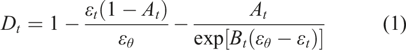
In this study, the theory of cracking in corroded reinforced concrete proposed by Wu (2013) was mainly adopted. In this theory, the concrete protective layer is simplified as a thick-walled concrete cylinder under the action of uniform corrosion of steel bar. The thick-walled cylinder idealization is widely adopted in analytical models of corrosion-induced cracking and has been validated against experimental data in numerous studies (Chang et al., 2024; Liang and Wang, 2020; Lu et al., 2011; Wang et al., 2016; Zhang et al., 2017; Zhao et al., 2021). This assumption is appropriate when the ratio of cover thickness to bar radius is not negligible, which is the case for typical reinforced concrete cover dimensions. However, it does not account for the influence of adjacent reinforcing bars, boundary effects near the concrete surface, or irregular cross-sectional geometries, which may introduce some deviation in practical applications. The assumption of uniform corrosion is a widely adopted simplification in analytical models of corrosion-induced cracking (Chang et al., 2024; Liang and Wang, 2020; Lu et al., 2011; Wang et al., 2016; Zhang et al., 2017; Zhao et al., 2021). Although non-uniform corrosion can occur in practice, the uniform corrosion assumption provides a tractable idealization that allows the corrosion expansion pressure and crack development to be described within a thick-walled cylinder framework. This simplification is particularly useful for structural assessment when detailed information on the actual corrosion morphology is unavailable. The corrosion expansion force is equated to a uniformly distributed radial internal pressure acting on the inner wall of the cylinder and inducing axisymmetric radial displacements. In the fully cracking stage, the concrete is all in the cracked zone. Since the cracks unfold in the radial direction, it is assumed that the modulus of elasticity of the concrete in the radial direction remains unchanged. The presence of cracks causes the modulus of elasticity in the circumferential direction to decrease (Zhao et al., 2016). In this study, the Mazars damage evolution theory (Mazars and Pijaudier, 1989) is used to describe the changes in the circumferential elastic modulus. In the Mazars damage model, two damage variables, D_t and D_c, are commonly used to describe tensile and compressive damage, respectively. Given that this paper investigates the process of corrosion cracking, the stresses on concrete are all tensile stresses, so this study only introduces the concept of the damage variable D_t to consider the damage of concrete in the radial direction. The evolution equation of the damage variable is obtained by fitting the experimental data as shown in the following equation. It can reflect the damage behavior of the material in different stress states:

D_{t} = 1 - \frac{ε_{t} (1 - A_{t})}{ε_{θ}} - \frac{A_{t}}{\exp [B_{t} (ε_{θ} - ε_{t})]}

(1)

where A_t, B_t are parameters determined from cylinder compression tests and beam bending tests;

ε_{θ}

is the circumferential strain;

ε_{t}

is the tensile strain. Therefore, the radial modulus of elasticity E_r satisfies the following relationship after damage due to corrosion.

E_{θ} = (1 - D_{t}) E_{r}

(2)

where

E_{θ}

is the circumferential modulus of elasticity. Coefficient is introduced from the above formula:

k = \frac{E_{θ}}{E_{r}} = 1 - D_{t}

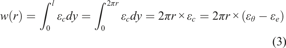
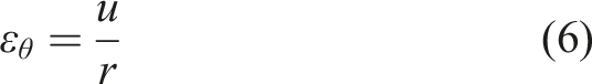
In this study, the concept of diffuse cracking is used in the modeling of concrete cracking (Long et al., 2008). The diffuse cracking concept treats the fracture process zone as a smeared band of microcracks rather than discrete cracks, which simplifies the mathematical treatment of crack width calculation. This assumption is reasonable for the fully cracked stage considered in this study, where multiple distributed cracks are present. However, it may lead to deviations in crack-width prediction in cases where localized macro-cracks dominate, and does not capture the discrete crack morphology observed in experimental specimens. The concept assumes that the fracture process area is a microfracture zone with a width of l. The microfractures are uniformly distributed along the width l of the fracture zone, and the conceptual diagram of diffuse fracture is shown in Figure 1. According to the concept of diffuse cracking, the circumferential strain at radius r (the total normal strain) is $ε_{θ}$ , elastic strain of concrete is $ε_{e}$ . Thus, the inelastic cracking strain at radius r is $ε_{c} = ε_{θ} - ε_{e}$ . Then the integration yields the crack width at radius r:

w (r) = \int_{0}^{l} ε_{c} d y = \int_{0}^{2 π r} ε_{c} d y = 2 π r \times ε_{c} = 2 π r \times (ε_{θ} - ε_{e})

(3)

where y is the crack normal coordinate. According to the elasticity theory, it is approximated that the elastic strain

ε_{e}

of the concrete in the fully cracked stage is:

ε_{e} = ε_{t} = f_{t} / E_{c}

(4)

where

ε_{t}

is the tensile strain of concrete, f _t the tensile strength of concrete, and E _c is the modulus of elasticity of concrete. For an anisotropic thick-walled cylinder subjected to axisymmetric action, the equilibrium differential, geometric, and physical equations (Li et al., 2006; Wu, 2013) are as follows: Equation (5) represents the radial equilibrium condition of the thick-walled cylinder, relating the spatial variation of radial stress to the difference between radial and circumferential stresses. Equations (6) and (7) are the geometric compatibility relations between strains and radial displacement. Equations (8) and (9) are the constitutive relations for the anisotropic damaged concrete, relating stresses to strains through the direction-dependent elastic moduli.

\frac{d σ_{r}}{d r} + \frac{σ_{r} - σ_{θ}}{r} = 0

(5)

ε_{θ} = \frac{u}{r}

(6)

ε_{r} = \frac{d u}{d r}

(7)

σ_{r} (r) = \frac{E_{c}}{1 - {ν_{c}}^{2}} [ε_{r} (r) + ν_{c} \sqrt{k} ε_{θ} (r)]

(8)

σ_{θ} (r) = \frac{E_{c}}{1 - {ν_{c}}^{2}} [k \cdot ε_{θ} (r) + ν_{c} \cdot \sqrt{k} \cdot ε_{r} (r)]

(9)

where

σ_{r}

is the circumferential stress,

σ_{θ}

is the tangential stress, u is the radial displacement, and

v_{c}

is the Poisson’s ratio. The Mohr-Coulomb yield criterion expressed in terms of radial and circumferential stresses with the inclusion of damage variables is (Zhao et al., 2011).

σ_{θ} = σ_{r} \frac{1 + (1 - D_{t}) \sin φ}{1 - (1 - D_{t}) \sin φ} + \frac{2 c \cos φ}{1 - (1 - D_{t}) \sin φ}

(10)

where D_t is the damage variable; c and φ are the cohesion and the angle of internal friction of the concrete, respectively.

Figure 1.

Diffuse crack modeling equivalent cracks.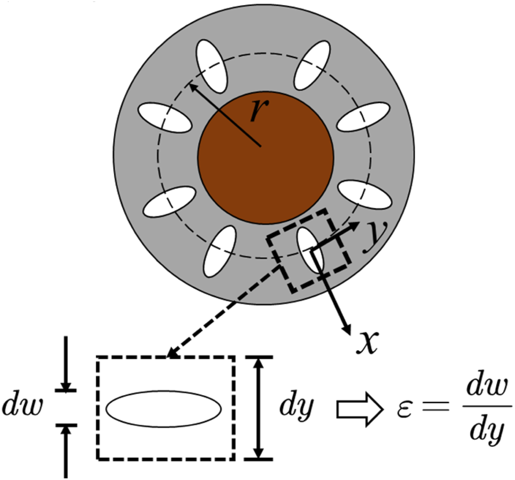

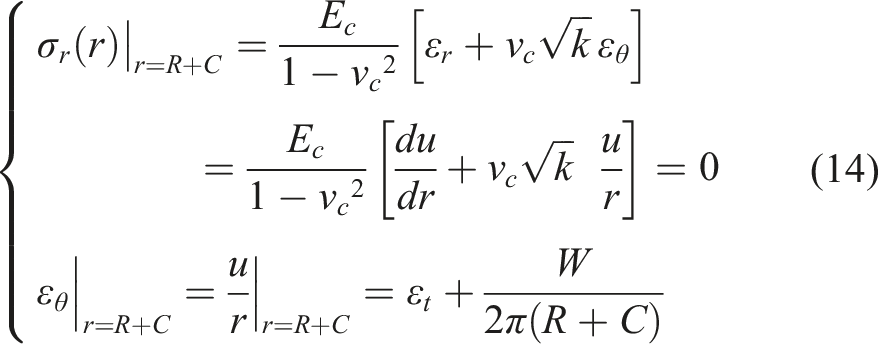
The stress control equation boundary conditions are.

{\begin{cases} σ_{r} |_{r = R + C} = 0 \\ ε_{θ} |_{r = R + C} = ε_{t} + \frac{W}{2 π (R + C)} \\ D_{t} = 1 - \frac{ε_{t} (1 - A_{t})}{ε_{θ} |_{r = R + C}} - \frac{A_{t}}{\exp [B_{t} (ε_{θ} |_{r = R + C} - ε_{t})]} \end{cases}

(11)

where W is the crack width on the surface of the concrete protection layer. The effect of radius variation on the damage variable D_t is ignored in this study. This simplification follows the theoretical framework adopted in previous corrosion-cracking models, where the damage variable is treated as an averaged parameter over the cracked concrete cover rather than a radius-dependent quantity. This assumption reduces the complexity of the governing equations while retaining the dominant effect of damage on the circumferential stiffness.

When r = R:

σ_{r} |_{r = R} = - q

(12)

where q is the corrosion expansion force acting on the inner wall of the concrete. If the crack width of the concrete surface is known, the corresponding expansion force q at this time can be obtained by using equations (5), (10)–(12).

The governing equation for the radial displacement is (Li et al., 2006):

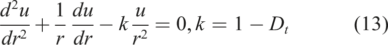
\frac{d^{2} u}{d r^{2}} + \frac{1}{r} \frac{d u}{d r} - k \frac{u}{r^{2}} = 0, k = 1 - D_{t}

(13)

The final expression for the boundary conditions of the displacement control equation is obtained by substituting the geometric relations into (11):

{\begin{cases} σ_{r} (r) |_{r = R + C} = \frac{E_{c}}{1 - {ν_{c}}^{2}} [ε_{r} + ν_{c} \sqrt{k} ε_{θ}] \\ = \frac{E_{c}}{1 - {ν_{c}}^{2}} [\frac{d u}{d r} + ν_{c} \sqrt{k} \frac{u}{r}] = 0 \\ ε_{θ} |_{r = R + C} = \frac{u}{r} |_{r = R + C} = ε_{t} + \frac{W}{2 π (R + C)} \end{cases}

(14)

Methodology

In this study, physics-guided probabilistic deep learning was proposed to complete the modeling of the cracking process of corroded reinforced concrete. Physics-guided probabilistic deep learning incorporates physical information, Bayesian theory and Deep Neural Networks. Thus, the following section is introduced from three parts: Deep Neural Networks (DNN), PINN, and physics-guided probabilistic deep learning.

DNN

DNN is a computational model consisting of multiple layers, including an input layer, several hidden layers, and an output layer. The tanh activation function is applied to introduce nonlinearity, with its output range of −1 to 1 keeping activations centered across layers, which contributes to the stability of the optimization process. The Mean Square Error (MSE) is used as the loss function (Li et al., 2024), optimized using the Adam algorithm (Kingma and Ba, 2015), which automatically adjusts the learning rate and performs well for sparse gradients.

Figure 2 illustrates the structure of the DNN, with input data denoted as (x₁, x₂, …, x_n) and the output as the predicted value, z. The fully connected DNN architecture is suitable for this problem because the corrosion cracking equations are formulated as functions of a single spatial variable r, and the target stress and displacement fields vary smoothly within the computational domain. Therefore, a compact fully connected network with tanh activation functions can provide sufficient nonlinear approximation capability while remaining computationally efficient. Since the input is one-dimensional, convolutional or recurrent structures are not required.

Figure 2.

Construction diagram of DNN.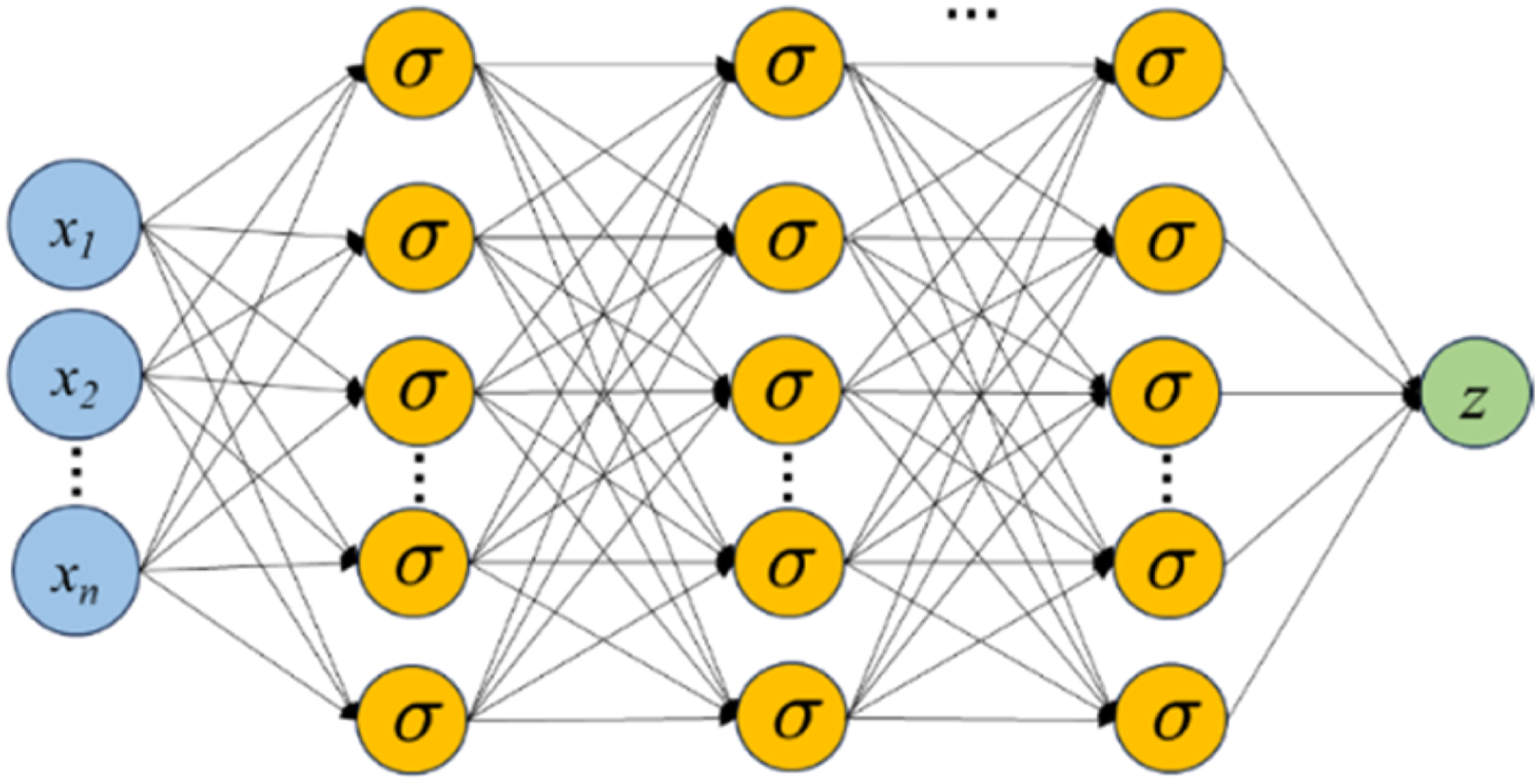

In this study, the specific network configurations are determined based on the stability analysis presented in Section 5. For the circumferential stress model, the network consists of 2 deterministic hidden layers and 1 probabilistic layer, with 50 neurons per hidden layer, trained for 20,000 epochs. For the radial displacement model, the network consists of 5 deterministic hidden layers with neurons configured as [10,50,100,20,20] and 1 probabilistic output layer, trained for 20,000 epochs. The tanh activation function is applied to all deterministic hidden layers in both models. The Adam optimizer is employed with a default learning rate of 0.001. Explicit regularization techniques such as dropout or L2 penalty are not applied. However, the KL divergence term in the variational inference objective implicitly regularizes the network weights by penalizing deviation from the prior distribution, as detailed in Section 3.3. All experiments were conducted on a laptop equipped with a 12th Gen Intel Core i5-1240P CPU, 16 logical processors, 1.70 GHz base frequency, and 16 GB RAM. No dedicated GPU was used, and all training was performed on the CPU. All network weights were initialized using the default Glorot uniform initializer (Xavier initialization), and biases were initialized to zero. The approximate training times were as follows: the PINN model for circumferential stress completed in less than 1 minute; the PINN model for radial displacement completed in approximately 20 minutes; and the physics-guided probabilistic deep learning models for circumferential stress and radial displacement each completed in approximately 30 minutes. The source code is available from the corresponding author upon reasonable request.

PINN

By directly embedding physical laws and constraints into the learning process, the PINN method can enhance the interpretability and generalization ability of the model, while reducing the need for large amounts of labeled training data (Bonfanti et al., 2023; Monaco and Apiletti, 2023; Zhang et al., 2024a). The construction diagram of PINN is shown in Figure 3. In this method, PINN is used to fit the solution z(x) at x, which is constrained by a physical model. The method learns the solution to the corroded reinforced concrete cracking equation in a self-supervised manner.

Figure 3.

Construction diagram of PINN.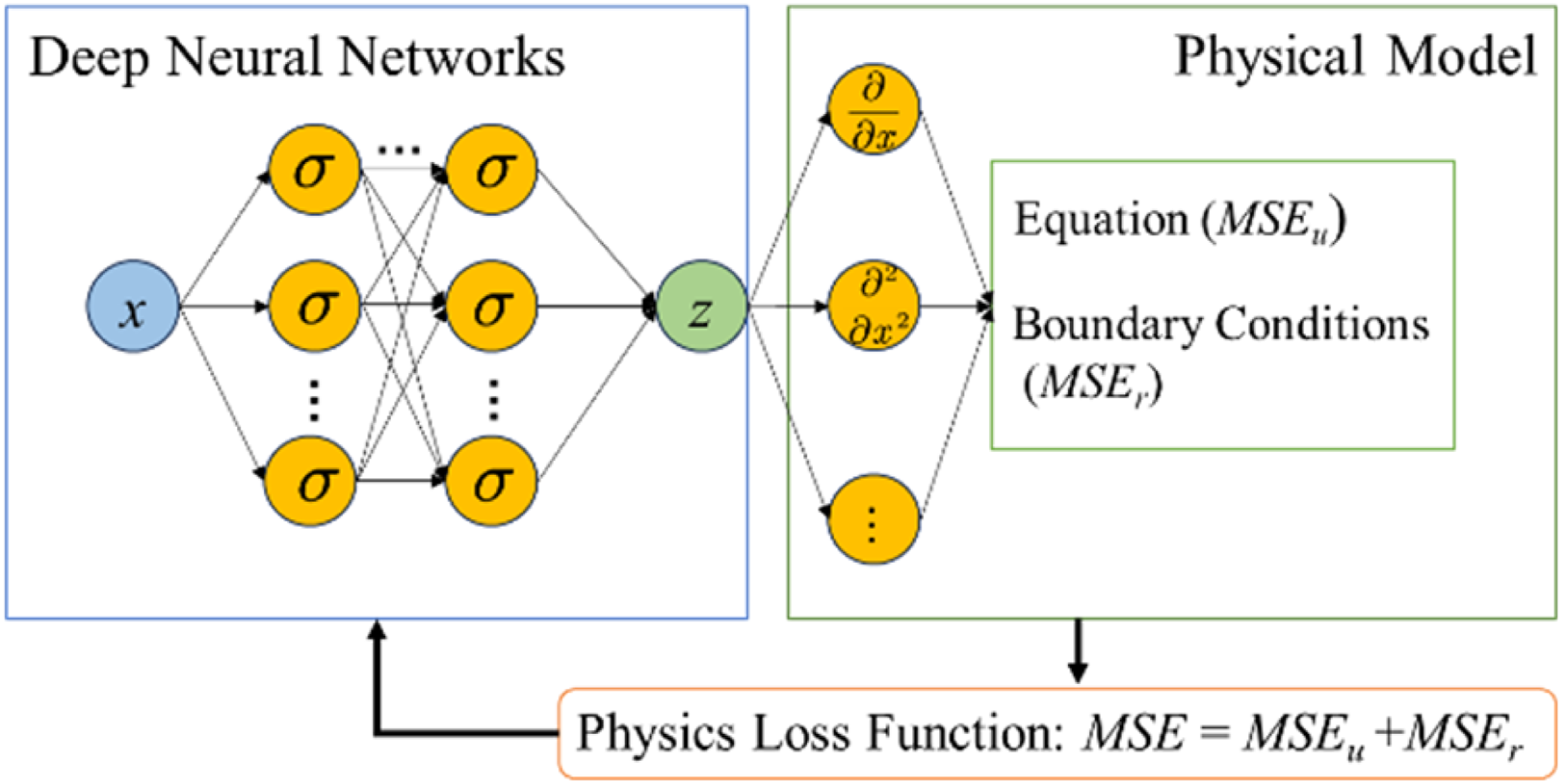

A series of data points (x) obtained by random sampling in the computational domain are used as inputs to the deep neural network. The number of neurons matches the feature dimensions of the data. However, in contrast to the supervised learning with true values in the previous section, PINN do not require true values as input. Thus, two physical constraints are added to the neural network to define the total loss function of the method in this paper as:

M S E = M S E_{u} + M S E_{r}

(15)

where MSE is the overall loss,

M S E_{u}

is the mean square error of the data points in the computational domain constrained by the equilibrium equations, and MSE_r is the mean square error of the data points in the boundary domain (r = R) constrained by the boundary conditions. In this study, equal weighting is applied to both loss components, i.e.,

M S E_{u}

and

M S E_{r}

are summed directly without additional coefficients. This is justified because both are mean squared errors over comparable collocation points, and Section 5 shows that the model achieves satisfactory convergence and accuracy under this scheme. The selection of optimal weighting strategies for physics-informed probabilistic models remains an open research question and is identified as a direction for future work.

Specifically, for the circumferential stress problem, $M S E_{u}$ is constructed from equations (5) and (10), which describe the equilibrium condition and the Mohr-Coulomb yield criterion within the domain R ≤ r ≤ R + C. At each collocation point, the neural network output and its spatial derivative are substituted directly into these equations, and the residual is minimized. $M S E_{r}$ is constructed from equations (11) and (12), which impose the stress boundary conditions at r = R and r = R + C. For the radial displacement problem, $M S E_{u}$ is constructed from equation (13), the governing second-order ordinary differential equation for radial displacement. The network output and its first- and second-order derivatives with respect to r are computed via automatic differentiation and substituted into equation (13) to form the residual. $M S E_{r}$ is constructed from equation (14), which enforces the displacement boundary condition at r = R + C. During training, minimizing the total loss MSE simultaneously drives the network solution to satisfy both the physical governing equations and the boundary conditions, without requiring any labeled solution data.

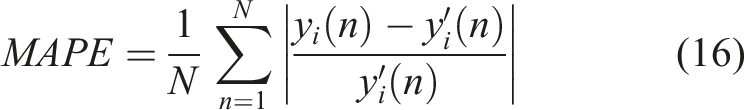
To evaluate the methodology of this paper, MAPE were used as the test metric (Behera et al., 2024). It is defined as follows:

M A P E = \frac{1}{N} \sum_{n = 1}^{N} | \frac{y_{i} (n) - y_{i}^{'} (n)}{y_{i}^{'} (n)} |

(16)

where N the number of samples in the test set,

y_{i}

(n) denotes the true value of the n^th sample, and

y_{i}^{'} (n)

denotes the predicted value of the n^th sample. Compared to traditional numerical methods such as finite element or finite difference approaches, PINNs offer several advantages for this problem. They do not require mesh generation and produce continuous differentiable solutions over the entire computational domain. Furthermore, they incorporate the governing physical equations directly into the training objective, eliminating the need for labeled solution data. However, PINNs are subject to known limitations. Training convergence can be sensitive to hyperparameter choices such as the number of collocation points, network depth, and the relative weighting of loss components. The selection of these parameters in this study is guided by the stability analysis presented in Section 5, which systematically evaluates their effects on model performance and provides practical recommended ranges.

Physics-guided probabilistic deep learning

The key idea behind physics-guided probabilistic deep learning is straightforward: instead of learning a single fixed set of network weights as in deterministic DNN or PINN, the proposed framework treats the weights as probability distributions. This allows the model to express uncertainty in its predictions. Specifically, regions where the physical constraints are weaker or less directly imposed tend to produce wider uncertainty intervals. The mathematical formulation below describes how this is implemented through Bayesian inference and variational inference.

In deterministic deep learning, methods such as backpropagation and gradient descent are typically used to update the weights and biases of neural networks to minimize a loss function. These weights and biases are fixed point estimates that do not take uncertainty into account. Thus, deterministic deep learning often fails to understand and quantify their own uncertainties in the solution process. However, in Bayesian Neural Networks (BNN), weights and biases are considered as random variables that obey some probability distribution (e.g., Gaussian distribution). This probability distribution reflects the uncertainty of these parameters. During training, the parameters of these probability distributions (mean and variance) are updated instead of the weights and biases themselves being directly updated (Zhang et al., 2024b). It is equivalent to ensemble an infinite number of neural networks on a certain weight distribution for prediction (Blundell et al., 2015). In order to quantitatively analyze the uncertainty of the output results, Bayesian theory and physical information neural network are combined in this paper to model the cracking process of corroded reinforced concrete.

The computational process of physics-guided probabilistic deep learning includes prior distribution selection, parameter posterior distribution calculation and prediction uncertainty estimation. $P (θ)$ is the prior of the network parameters as well as the unknown terms in the differential equation, and a Gaussian distribution is generally chosen as the prior distribution. Gaussian distribution can well describe the uncertainty of data and is widely used in practice. The mean (µ) and variance (σ²) of the prior distribution are generally determined by prior knowledge and domain properties. The Gaussian distribution is chosen as the prior because it is mathematically convenient, widely used in Bayesian neural networks, and compatible with variational inference implementations. In addition, a zero-mean Gaussian prior acts as an implicit L2 regularizer on the network weights, penalizing excessively large weight values and reducing the risk of overfitting, which is particularly beneficial when the number of collocation points is limited.

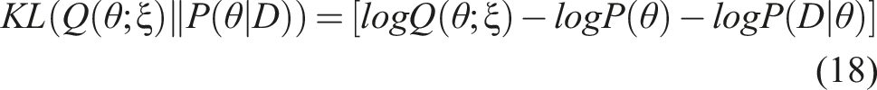
For parameter posterior distribution calculation, according to Bayesian theory, the posterior distribution of weights in physics-guided probabilistic neural networks is generally defined as: $P (θ | D)$ . $P (D | θ)$ represents the likelihood of the dataset D. D includes D_z, D_f, D_r three components. D_z includes the physically guided probabilistic deep learning fit z(x) and its corresponding value x. D_f includes the forcing term f of the control equation and its counterpart x. D_r includes the boundary value r and its counterpart x (Yang et al., 2021). Then, the likelihood can be calculated as:

P (D | θ) = P (D_{z} | θ) P (D_{f} | θ) P (D_{r} | θ)

(17)

This posterior distribution is the value to be inferred, but this is difficult for the vast majority of neural networks. Methods for the computation of posterior distributions include Markov Chain Monte Carlo (MCMC) methods, importance sampling, and approximate Bayesian computation methods (Gelman et al., 2013). Among them, Variational Inference (VI) is one of the most effective and more efficient methods to compute the posterior distribution, which approximates the true posterior distribution by approximating a set of parameters of the posterior distribution (Gelman et al., 2013). In the VI method, we approximate the posterior density $P (θ | D)$ of the unknown parameter vector $θ$ with another density function Q (θ;ξ). VI transforms the inference of the posterior distribution of the parameter into an optimization problem based on the principle of variational lower bounding (Graves, 2011). The Kullback-Leibler scattering (KL) is used to measure the proximity of the two distributions. The closer the distributions are, the smaller KL is (Belov and Armstrong, 2011). Unlike deterministic deep learning, physics-guided probabilistic deep learning is to optimize the parameter ξ to maximize the similarity of the two distributions, i.e., to minimize the KL between the two distributions. The Adam optimizer is often used to update ξ to minimize the loss. The conversion of the KL is as follows:

K L (Q (θ; ξ) ‖ P (θ | D)) = [l o g Q (θ; ξ) - l o g P (θ) - l o g P (D | θ)]

(18)

In this way, the BNN is combined with the physical information. The network architecture is illustrated in Figure 4.

Figure 4.

Architecture of physics-guided probabilistic deep learning.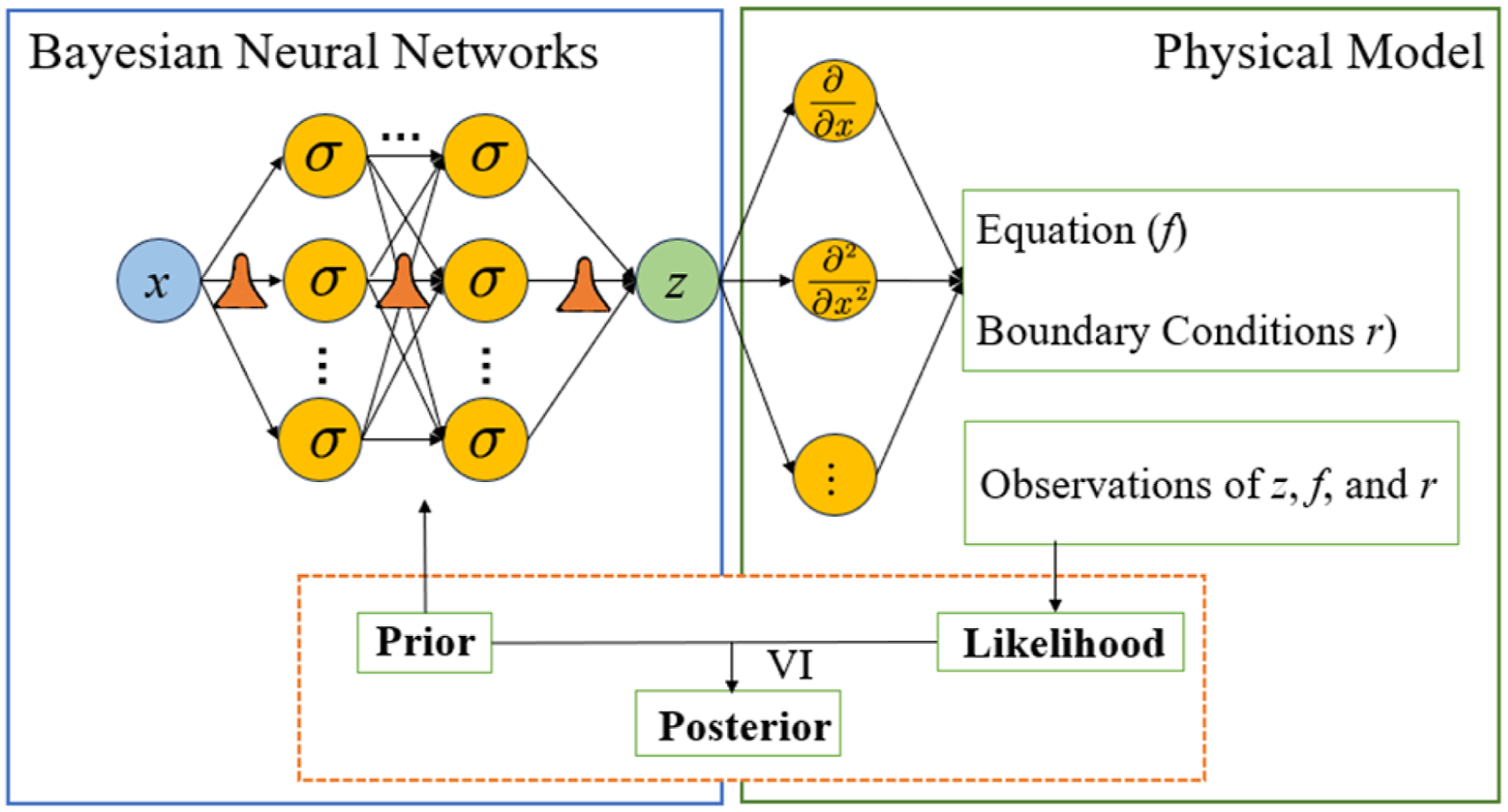

In the standard training process of deep learning, backpropagation algorithms are usually utilized to compute the gradient and update the network parameters to minimize the loss function. When it comes to weights sampled from the posterior distribution, it becomes difficult to directly perform differentiation operations on these samples because the sampling process itself is usually not differentiable. This means that one cannot simply apply the standard backpropagation algorithm directly to randomly chosen weight samples to compute the gradient. To overcome this difficulty, reparameterization techniques (Kingma and Welling, 2013) and Flipout methods (Wen et al., 2018) can be applied. Reparameterization techniques convert the process of sampling random variables into a sampling problem with derivable parameters. Specifically, the random weights are represented as a combination of a deterministic function and a random variable with a fixed distribution (e.g., standard normal distribution). For example, z, which was originally sampled from N (x, ϕ²), can be converted to sampling ε from the standard normal distribution N (0, 1) and then obtaining z by means of z = x + ε ⋅ ϕ. In this way, the sampling process is converted to the sampling of x and ϕ, which are derivable parameters, and thus they can be updated using a gradient descent algorithm. The Flipout method is an efficient weight transformation technique that enables near-independent weight transformations in small batches. Specifically, Flipout introduces randomness by “flipping” each weight randomly without adding additional computational burden. This “flipping” process can be accomplished by sampling the weights and adding them to the network, thus making better use of stochasticity in the computation of the gradient and improving the efficiency of the gradient estimation. In the section on modeling stability analysis of cracking in corroded reinforced concrete, a comparative analysis of the effects of the two methods in this study is presented.

In this framework, uncertainty in the model predictions stems from the probabilistic treatment of the network weights. Rather than assigning fixed values to the weights, the proposed framework models them as probability distributions, whose parameters are optimized through VI as described above. Once the posterior distribution of the network weights is approximated, uncertainty is propagated to the model predictions via Monte Carlo sampling. Specifically, the network weights are sampled repeatedly from the approximated posterior distribution, and a forward pass is performed for each sample. In this study, 1000 forward passes are conducted for each input point, yielding an ensemble of predictions from which the mean and standard deviation are computed. The mean serves as the point estimate of the predicted quantity, while the standard deviation characterizes the prediction uncertainty. The 95% predictive uncertainty interval is approximated as the mean ±1.96 standard deviations, assuming an approximately normal predictive distribution. The validity of the uncertainty estimates is assessed in the section on modeling performance analysis of cracking in corroded reinforced concrete by examining whether the theoretical values fall within the predicted confidence intervals across the computational domain. This provides a practical assessment of whether the predicted uncertainty bounds are consistent with the reference theoretical solutions.

Compared to deterministic PINN, the proposed framework offers two additional capabilities. First, it provides quantified prediction uncertainty, enabling engineers to assess the reliability of the predicted corrosion expansion force and radial displacement rather than relying solely on point estimates. Second, the Bayesian framework incorporates prior knowledge through the prior distribution, which acts as a regularizer and helps stabilize training when the number of collocation points is limited.

Modeling performance analysis of cracking in corroded reinforced concrete

In order to mention the feasibility and performance of the method, a practical arithmetic example was used for validation (Zhao et al., 2011). The calculation parameters were: the diameter of the steel-bar d = 20 mm; tensile strength of concrete f _t = 2.2 MPa; thickness of the protective layer C = 35 mm; modulus of elasticity E _c = $3.15 \times 10^{4}$ MPa; Poisson’s ratio v _c = 0.2; cohesion c = 3 MPa; angle of internal friction $φ = 55 °$ ; the coefficients of the Mazars model $A_{t} = 0.7$ and $B_{t} = 10000$ . The above parameters were substituted into the stress, and radial displacement equations. Then the equations were embedded into the algorithm. Thus, the modeling of the cracking process of corroded reinforced concrete was completed. The above parameters are derived from experimental values (Zhao et al., 2011). All the theoretical values of the circumferential stress and radial displacement mentioned in this study refer to the values obtained by analytical solution methods. Instead of dividing the training and test sets, it is only necessary to design the sampling points to be solved in the physical domains R to R + C.

The theoretical model adopted in this study is directly derived from the analytical framework proposed by Zhao et al. (2011) and Wu (2013), which integrates damage mechanics and the Mazars damage model to describe the corrosion-induced cracking process. The model was verified against experimental measurements of steel-bar radial loss at concrete surface cracking from multiple independent experimental programs, demonstrating reasonable agreement with test data. The analytical solutions generated by this verified framework serve as the reference values for evaluating the performance of the proposed physics-guided probabilistic deep learning approach in the present study.

PINN-based modeling performance analysis

By assuming different values for the surface crack width, the variation curve of circumferential stress with the inner radius of the steel bar was obtained, as shown in Figure 5. All the theoretical values mentioned in this study refer to the values obtained by analytical solution methods. In this section, PINN was used to complete the modeling of the cracking process of corroded reinforced concrete.

Figure 5.

Fitting effects of PINN (circumferential stress). (a) W = 0.06 mm; (b) W = 0.1 mm; (c) W = 0.2 mm; (d) W = 0.3 mm; (e) W = 0.4 mm; (f) W = 0.5 mm.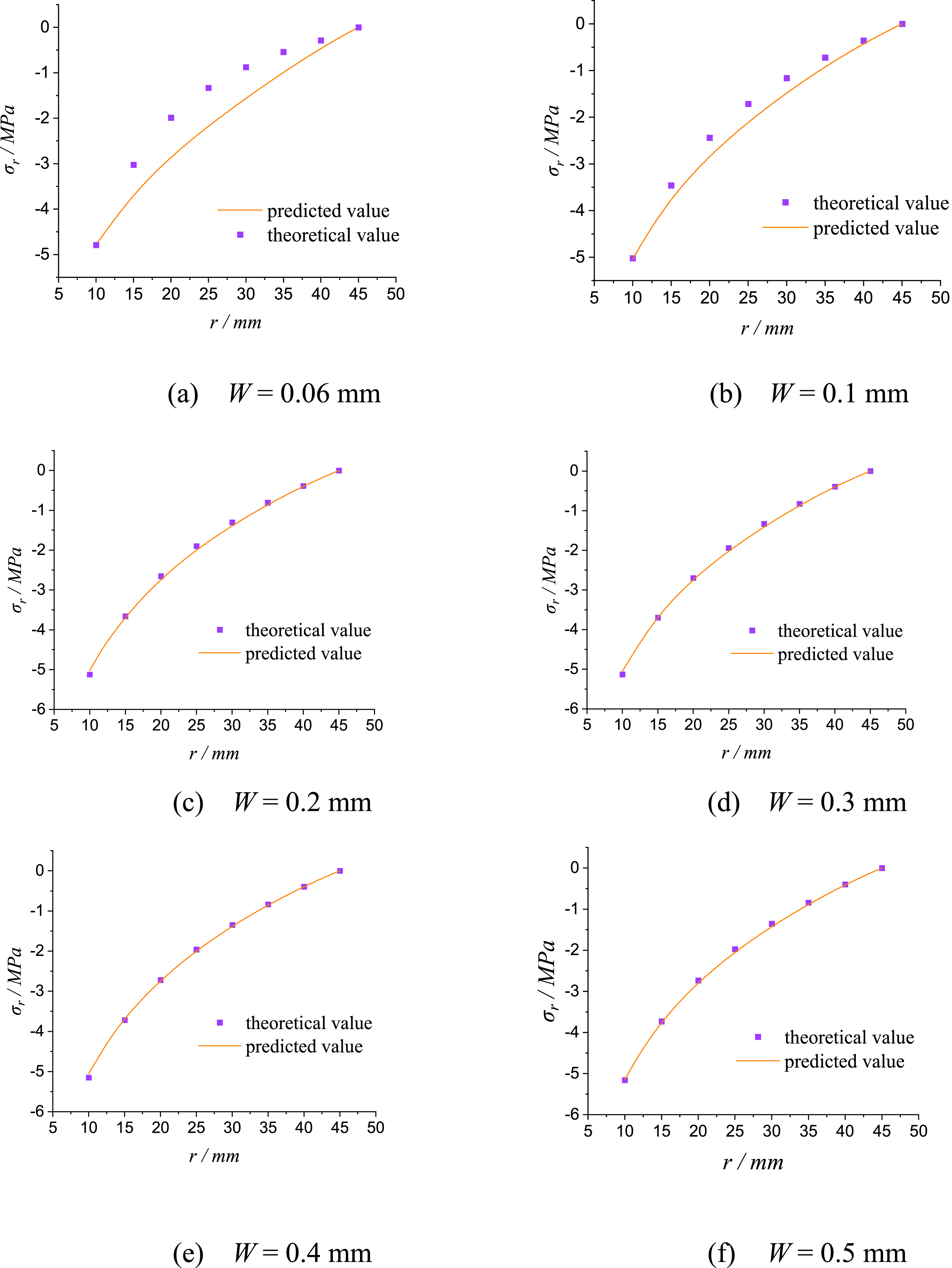

The important hyperparameters in PINN are listed below: the number of hidden layers setting as 2; the number of hidden layer neurons setting as 50; the number of training samples as 20; the number of epochs setting as 2000. The circumferential stresses increased with the inner radius, but the rate of increase slowed down with growth. The fit to the boundary values was accurate regardless of the change in W (crack width on the surface of the concrete protection layer), while the intermediate fitting values were a little off at the small values of W. This was because the control conditions were at the boundary points.

By assuming different values for the surface crack width, the variation curve of displacement with the inner radius of the steel bar was obtained, as shown in Figure 6. The important hyperparameters in PINN are listed below: the hidden layer of the neural network as 6 layers; the number of neurons in the hidden layer as 10,50,100,20,20,1; the number of training samples as 50; the number of epochs as 20,000. The fitted values of the displacements at r = 45 are very accurate at different surface crack widths, however, the fitted values at r = 10 are somewhat deviated. This is because the points controlled by the control equations in this study are all at r = 45. This phenomenon also reveals the sensitivity of the model fit at different locations. Since the PINN model relies on the control equations to guide the training of the solution, the region covered by the control equations directly affects the model fitting. To address this issue, future research could consider adding more control points, especially in the low-radius region, to improve the model’s performance throughout the computational domain.

Figure 6.

Fitting effects of PINN test set (radial displacement). (a) W = 0.06 mm; (b) W = 0.10 mm; (c) W = 0.20 mm; (d) W = 0.30 mm; (e) W = 0.40 mm; (f) W = 0.50 mm.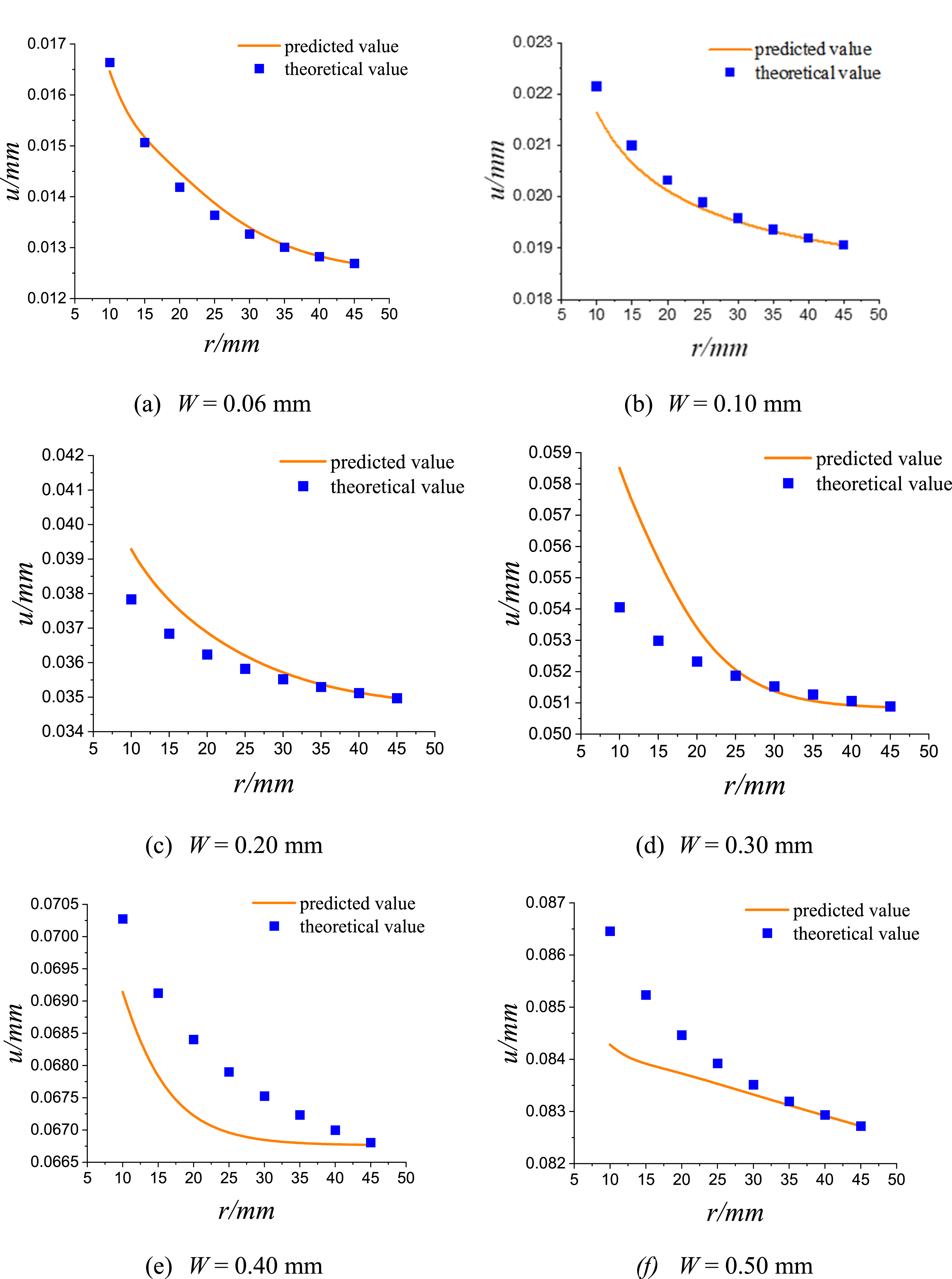

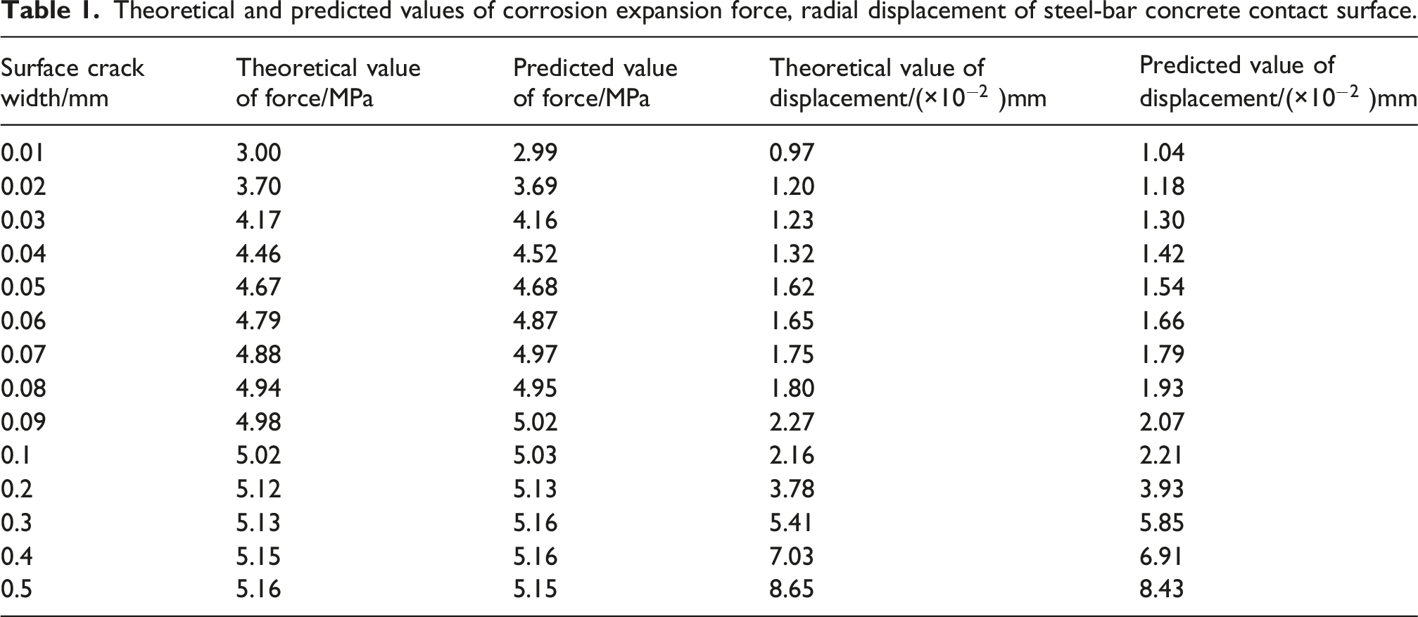
In this study, the surface crack width was assumed, and then the corresponding circumferential stress value at the specific inner radius was obtained based on PINN. According to the boundary condition equation (12), the opposite of the value of the circumferential stress at r = 10 can be known as the corrosion expansion force. The comparison between the theoretical and predicted values of the corrosion expansion force and radial displacement of the steel-bar concrete contact surface obtained accordingly is shown in Table 1. In order to visualize the comparison, the theoretical and predicted values for the values are shown in Figure 7. The MAPE of corrosion expansion force and radial displacement of the steel-bar concrete contact surface were 0.58% and 4.6%, respectively. According to the relevant theoretical and empirical formulas, the values of steel-bar consumption raw material, critical corrosion expansion cracking time, steel-bar mass corrosion rate, and steel-bar corrosion depth can be further obtained from the radial displacement of the steel-bar concrete contact surface (Pantazopoulou and Papoulia, 2001; Zhao and Jin, 2006).

Table 1.

Theoretical and predicted values of corrosion expansion force, radial displacement of steel-bar concrete contact surface.

Surface crack width/mm	Theoretical value of force/MPa	Predicted value of force/MPa	Theoretical value of displacement/( $\times 1 0^{- 2}$ )mm	Predicted value of displacement/( $\times 1 0^{- 2}$ )mm
0.01	3.00	2.99	0.97	1.04
0.02	3.70	3.69	1.20	1.18
0.03	4.17	4.16	1.23	1.30
0.04	4.46	4.52	1.32	1.42
0.05	4.67	4.68	1.62	1.54
0.06	4.79	4.87	1.65	1.66
0.07	4.88	4.97	1.75	1.79
0.08	4.94	4.95	1.80	1.93
0.09	4.98	5.02	2.27	2.07
0.1	5.02	5.03	2.16	2.21
0.2	5.12	5.13	3.78	3.93
0.3	5.13	5.16	5.41	5.85
0.4	5.15	5.16	7.03	6.91
0.5	5.16	5.15	8.65	8.43

Figure 7.

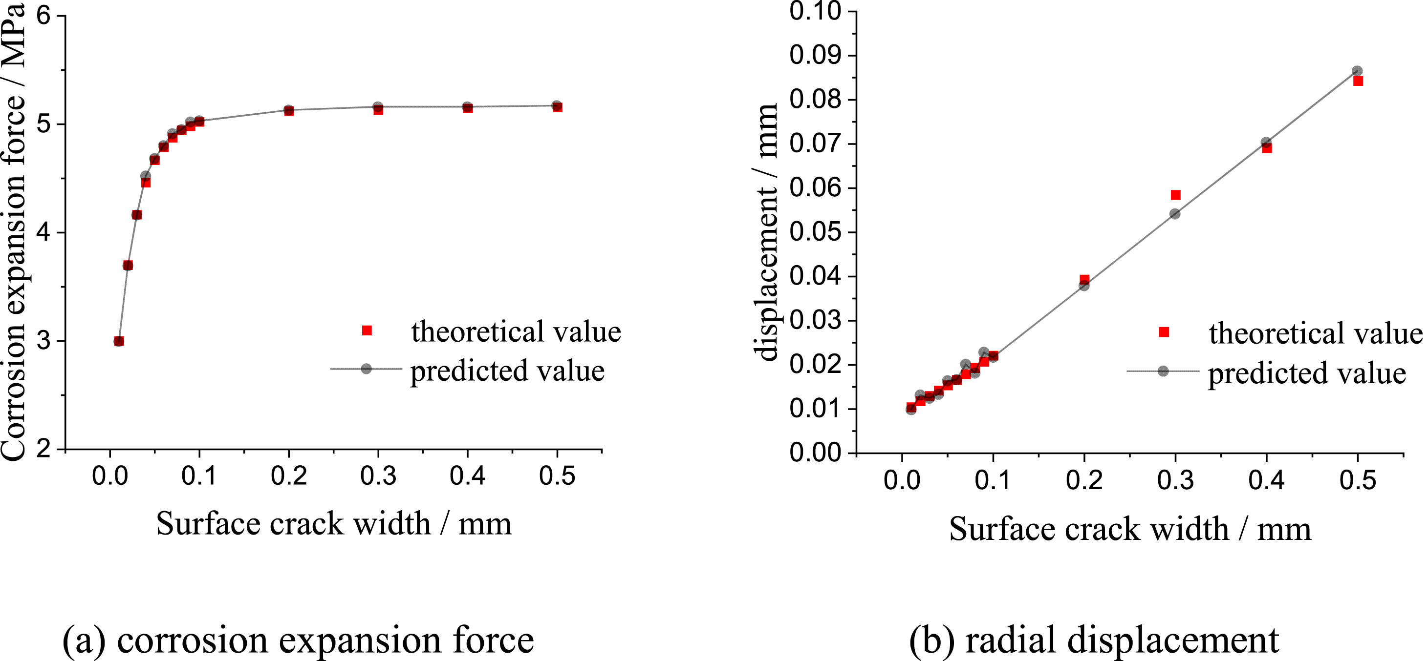
Comparison of theoretical and predicted values of PINN. (a) Corrosion expansion force; (b) Radial displacement.

Physics-guided probabilistic deep learning-based modeling performance analysis

In this subsection, the physics-guided probabilistic deep learning was used to analyze the uncertainty of the output results quantitatively. The curve of the process of circumferential stress variation with the inner radius of the steel-bar and the uncertainty of the prediction is shown in Figure 8 below. The closer the point was to the control point (r = 45) the lower the uncertainty was, for the reason that control equations controlled the point at the value at r = 45. The boundary loss term $M S E_{r}$ explicitly constrains the network output at r = 45 during training, effectively anchoring the prediction and reducing the admissible solution space near this location. As a result, the posterior predictive distribution becomes more concentrated near the constrained boundary point, leading to narrower uncertainty intervals. The important hyperparameters are listed below: the number of hidden layers as 2, the number of probabilistic layers as 1, the number of neurons in the hidden layer as 50, the number of training samples as 50, the number of epochs as 20,000, and the gradient descent algorithm as the reparameterization algorithm.

Figure 8.

Fitting effects of physics-guided probabilistic deep learning (circumferential stress). (a) W = 0.06 mm; (b) W = 0.1 mm; (c) W = 0.2 mm; (d) W = 0.3 mm; (e) W = 0.4 mm; (f) W = 0.5 mm.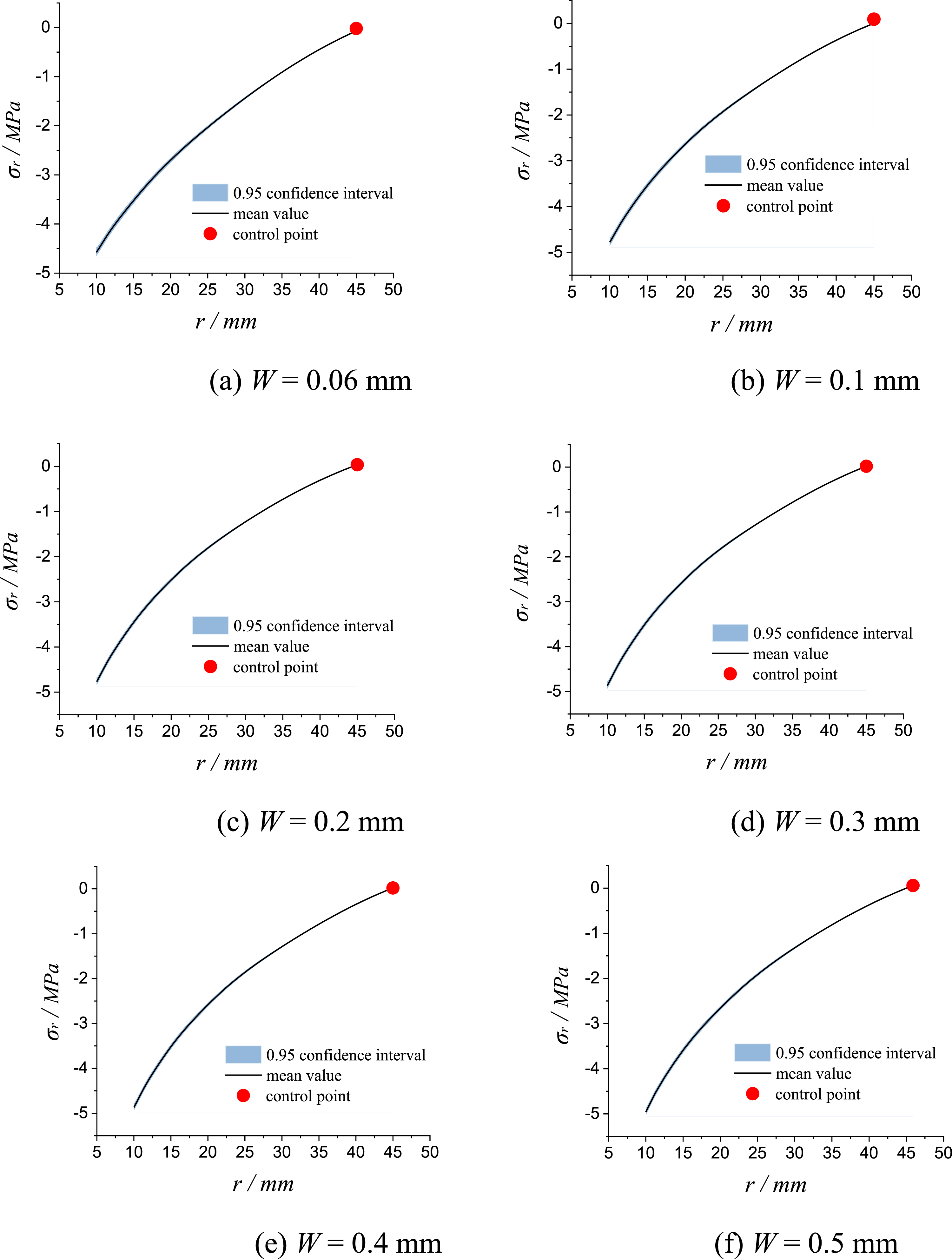

The important hyperparameters for predicting the radial displacement in physics-guided probabilistic deep learning are listed below: the hidden layer of the neural network as 6; the number of neurons in the hidden layer as 10,50,100,20,20,1; the number of probabilistic layers as 1; the number of training samples as 50; the number of epochs as 20,000; the gradient descent algorithm as the reparameterization algorithm. The curve of the process of radial displacement variation with the inner radius of the steel-bar and the uncertainty of the prediction is shown in Figure 9 below. With this approach, not only the predicted values of the output results are obtained, but also the uncertainty of these predicted values is quantified, thus providing more reliable information for practical applications. However, the fitting of the model performed better in the vicinity of the control points, while the fitting decreased in the region away from the control points. To improve this, increasing the number of control points or adding more boundary constraints should be considered in the future research. A similar pattern is observed for the radial displacement predictions, where uncertainty also decreases near the boundary point r = R + C, for the same reason as described above.

Figure 9.

Fitting effects of physics-guided probabilistic deep learning (radial displacement). (a) W = 0.06 mm; (b) W = 0.1 mm; (c) W = 0.2 mm; (d) W = 0.3 mm; (e) W = 0.4 mm; (f) W = 0.5 mm.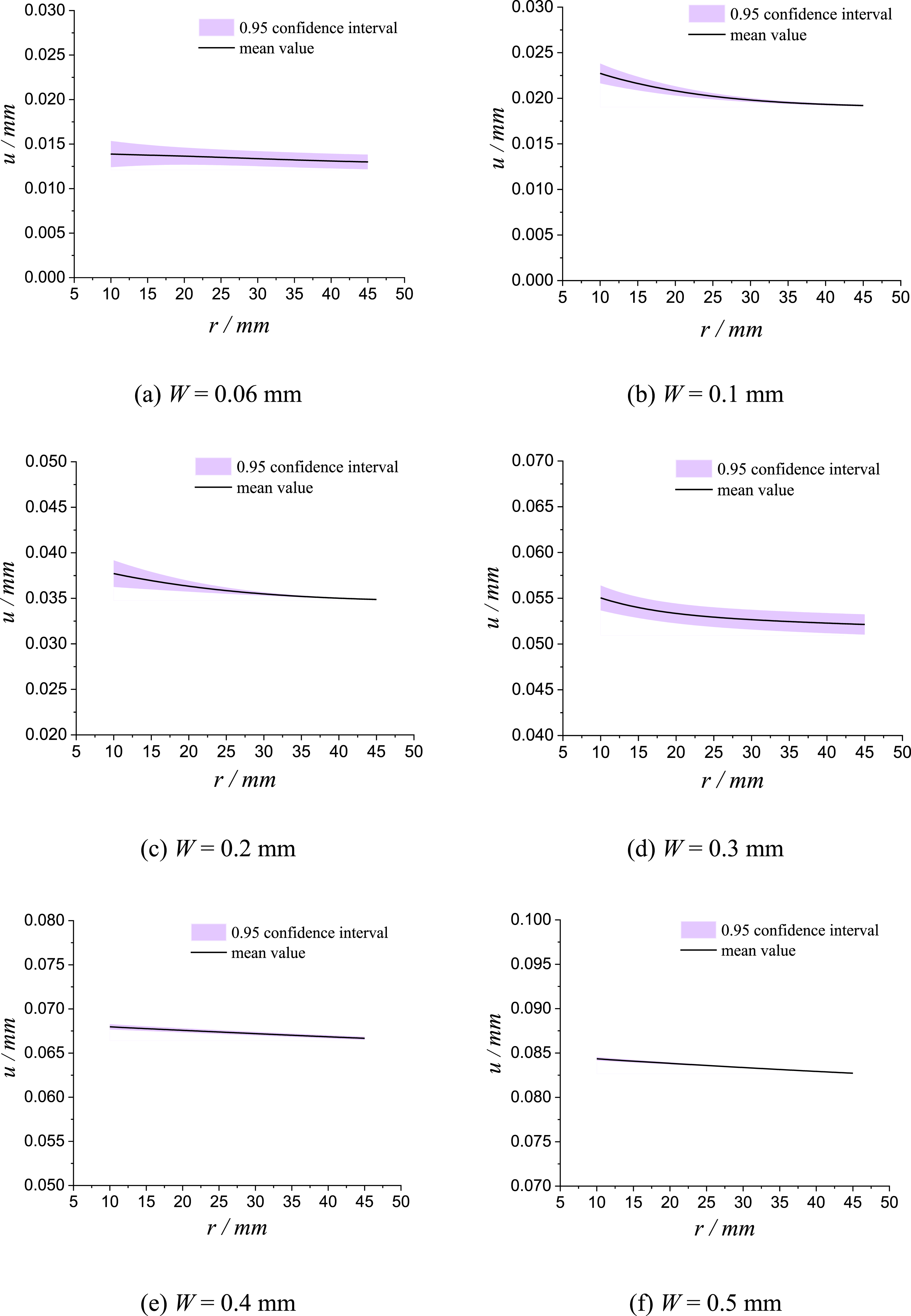

In this study, the corrosion expansion force and radial displacement at the steel-bar concrete contact surface, as predicted by physics-guided probabilistic deep learning, were evaluated. The predicted values were then compared with the theoretical values, as shown in Figure 10. The physics-guided probabilistic deep learning predicted the approximate range of the corrosion expansion force and radial displacement. It can be seen that the theoretical values are almost within the predicted range. It was superior to PINN in performance and generalization. The uncertainty quantified in this framework is primarily epistemic in nature, arising from finite collocation points, limited boundary constraints, and uncertainty in the learned network parameters. Aleatory uncertainty associated with intrinsic material variability, corrosion randomness, or measurement noise is not explicitly modeled in the current framework. The improvement of physics-guided probabilistic deep learning over deterministic PINN is not limited to the provision of uncertainty intervals. While PINN produces a single point estimate for each predicted quantity, the proposed framework provides a full predictive distribution, which enables a more informative assessment of model reliability. In particular, the narrower uncertainty intervals observed near the boundary point r = R + C reflect the stronger constraint imposed by the boundary loss term, whereas the wider intervals in the interior of the domain indicate regions where the model relies more heavily on the governing equations rather than direct boundary anchoring. This spatially varying uncertainty pattern provides engineers with location-specific confidence information that is not available from deterministic PINN predictions.

Figure 10.

Comparison of theoretical and predicted values of physics-guided probabilistic deep learning. (a) Corrosion expansion force; (b) Radial displacement.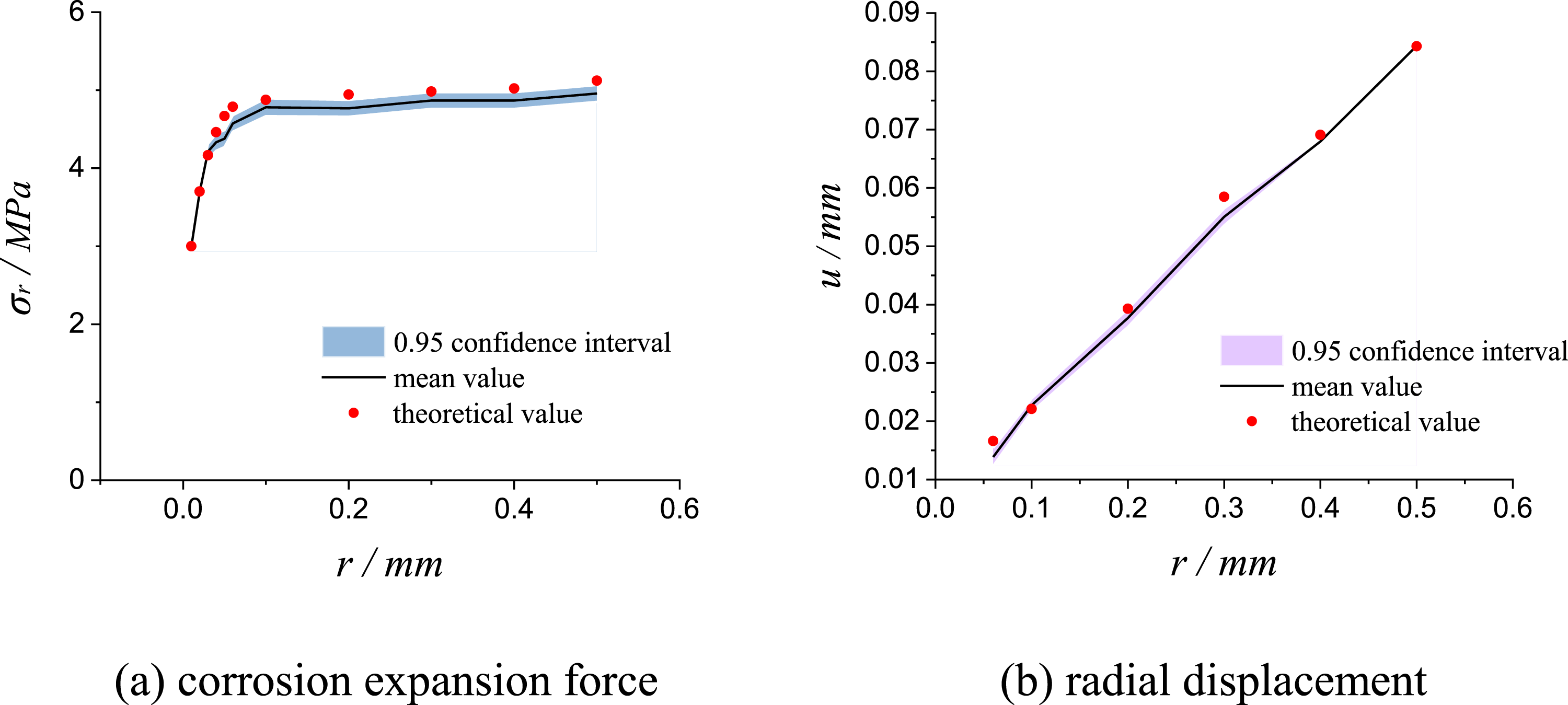

Modeling stability analysis of cracking in corroded reinforced concrete

PINN-based modeling stability analysis

Stability analysis of circumferential stress fitting

Factors affecting the fitting effectiveness of PINN include the number of hidden layers of the neural network (HL), the number of neurons in the hidden layer (NH), and the number of training samples (TS) etc. In order to explore the effect of TS, the cracking process was modelled when W was 0.5 mm, HL was 2, and NH was 50. The samples were uniformly sampled in an interval from 10 to 60 mm radius. TS was transformed, and the gap between the circumferential stress fitting effect and the theoretical value was compared, which is shown in Table 2. When the TS was too small or too large, the neural network performance was poor, and the MAPE were over 0.05. In order to visualize the prediction effect, the predicted and theoretical values under different TS are shown in Figure 11(a). It is obvious that when the TS was too small or too large, the fitted curves are all far from the theoretical value. So, the recommended interval for TS is 10 - 100, and the MAPE of this interval is within 0.03. When TS is too small, the network has insufficient collocation points to learn the spatial variation of the governing equations, leading to underfitting. When TS is too large, the increased density of points does not provide additional information beyond what the physical equations already constrain, and may introduce numerical instability during training.

Table 2.

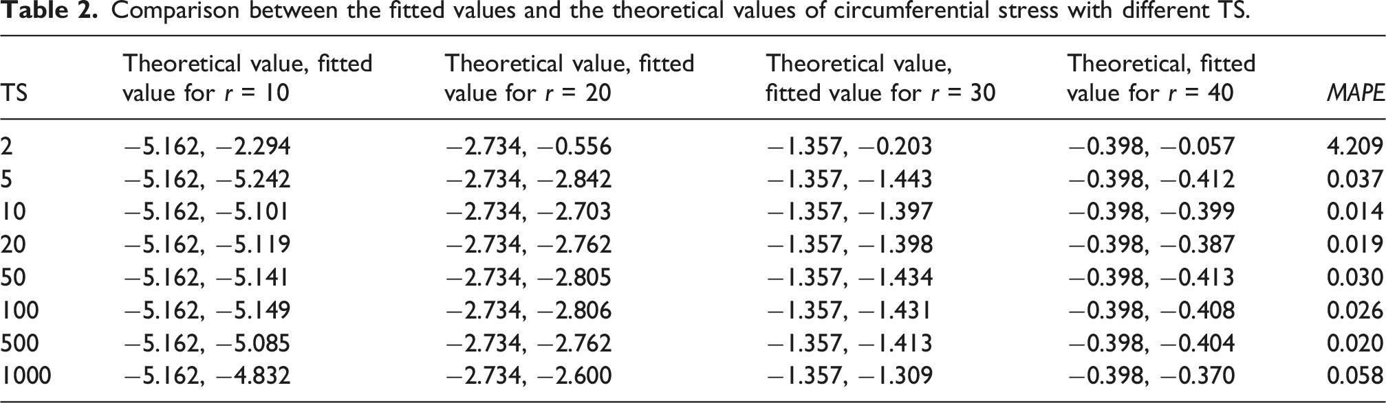
Comparison between the fitted values and the theoretical values of circumferential stress with different TS.

TS	Theoretical value, fitted value for r = 10	Theoretical value, fitted value for r = 20	Theoretical value, fitted value for r = 30	Theoretical, fitted value for r = 40	MAPE
2	−5.162, −2.294	−2.734, −0.556	−1.357, −0.203	−0.398, −0.057	4.209
5	−5.162, −5.242	−2.734, −2.842	−1.357, −1.443	−0.398, −0.412	0.037
10	−5.162, −5.101	−2.734, −2.703	−1.357, −1.397	−0.398, −0.399	0.014
20	−5.162, −5.119	−2.734, −2.762	−1.357, −1.398	−0.398, −0.387	0.019
50	−5.162, −5.141	−2.734, −2.805	−1.357, −1.434	−0.398, −0.413	0.030
100	−5.162, −5.149	−2.734, −2.806	−1.357, −1.431	−0.398, −0.408	0.026
500	−5.162, −5.085	−2.734, −2.762	−1.357, −1.413	−0.398, −0.404	0.020
1000	−5.162, −4.832	−2.734, −2.600	−1.357, −1.309	−0.398, −0.370	0.058

Figure 11.

Comparison of the effects of different factors on the performance of neural networks (stress). (a) TS; (b) NH; (c) HL.

In order to explore the effect of NH, the cracking process was modelled when W was 0.5 mm, HL was 2, and TS was 20. NH was changed. The circumferential stress fitting effect with the theoretical values are compared, as shown in Table 3. When the NH was too small (2 or 5), the neural network did not learn the laws of differential equations well, and the MAPE values in this interval were all more than 100. However, when the NH was too large (1000 neurons), the neural network also performed badly. It was not only slow in training speed, but also occurred overfitting phenomenon. In order to visualize the prediction effect, the predicted and theoretical values under different NH are shown in Figure 11(b). It is obvious that when the NH was too small or too large, the fitted curves are all far from the theoretical value. Therefore, it is recommended that the NH should be in the range of 10 to 50, and the MAPE value in this range will be within 0.03. When NH is too small, the network lacks sufficient capacity to represent the nonlinear stress distribution, resulting in poor approximation. When NH is too large, the increased model complexity leads to overfitting of the collocation points rather than learning the underlying physical behavior, which manifests as degraded generalization.

Table 3.

Comparison between the fitted values and the theoretical values of circumferential stress with different NH.

NH	Theoretical value, fitted value for r = 10	Theoretical value, fitted value for r = 20	Theoretical value, fitted value for r = 30	Theoretical value, fitted value for r = 40	MAPE
2	−5.162, −0.00012	−2.734, −0.00012	−1.357, −0.00012	−0.398, −0.00012	20,105.250
5	−5.162, −1.847	−2.734, −0.211	−1.357, −0.00877	−0.398, 0.000745	175.678
10	−5.162, −5.147	−2.734, −2.800	−1.357, −1.429	−0.398, −0.408	0.025
20	−5.162, −5.008	−2.734, −2.672	−1.357, −1.340	−0.398, −0.385	0.025
50	−5.162, −5.043	−2.734, −2.721	−1.357, −1.375	−0.398, −0.397	0.011
100	−5.162, −5.168	−2.734, −2.799	−1.357, −1.387	−0.398, −0.349	0.047
500	−5.162, −5.113	−2.734, −2.697	−1.357, −1.312	−0.398, −0.366	0.036
1000	−5.162, −4.838	−2.734, −2.321	−1.357, −0.996	−0.398, −0.252	0.297

In order to explore the effect of HL, the cracking process was modelled when W was 0.5 mm, TS was 20, and NH was 50. HL was transformed to compare the circumferential stress fitting effect with the theoretical value, as shown in Table 4. The HL had no significant effect on the fitting effect of the neural network, and the MAPE value was within 0.05. It is also visually shown in Figure 11(c). However, the increase in the HL significantly increased the training time, thus the interval of HL is recommended to be 2–20 for the efficiency of training. The relatively weak sensitivity of model performance to HL suggests that the circumferential stress problem can be adequately represented by shallow networks, as the governing equations involve smooth functions of a single spatial variable. Deeper networks increase computational cost without providing meaningful improvement, consistent with the principle of parsimony in model selection.

Table 4.

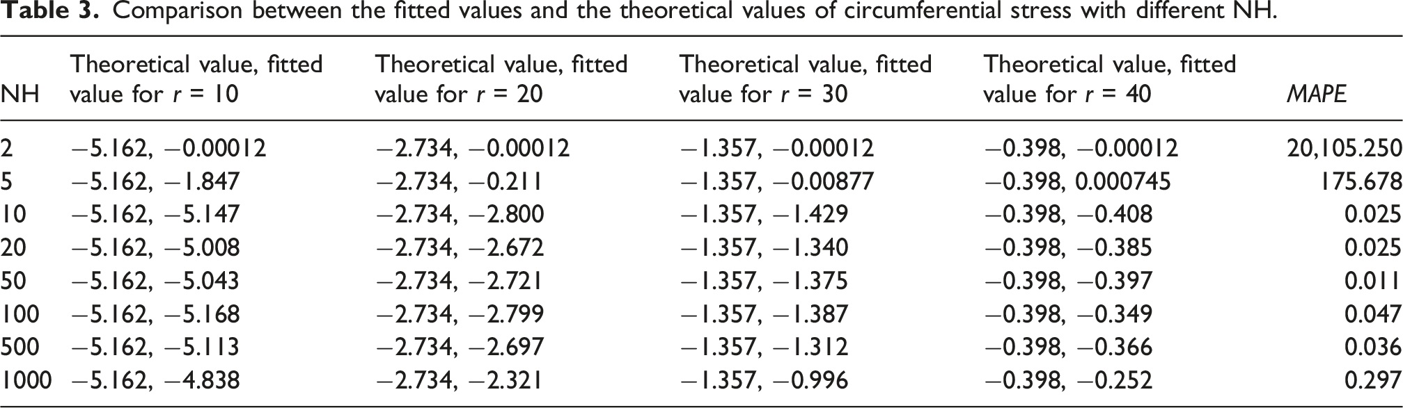
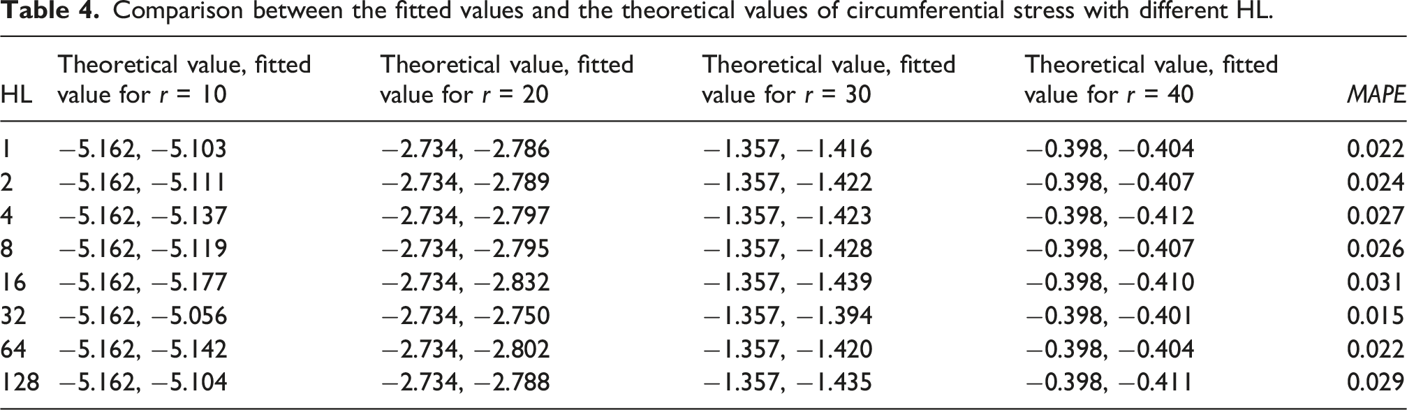
Comparison between the fitted values and the theoretical values of circumferential stress with different HL.

HL	Theoretical value, fitted value for r = 10	Theoretical value, fitted value for r = 20	Theoretical value, fitted value for r = 30	Theoretical value, fitted value for r = 40	MAPE
1	−5.162, −5.103	−2.734, −2.786	−1.357, −1.416	−0.398, −0.404	0.022
2	−5.162, −5.111	−2.734, −2.789	−1.357, −1.422	−0.398, −0.407	0.024
4	−5.162, −5.137	−2.734, −2.797	−1.357, −1.423	−0.398, −0.412	0.027
8	−5.162, −5.119	−2.734, −2.795	−1.357, −1.428	−0.398, −0.407	0.026
16	−5.162, −5.177	−2.734, −2.832	−1.357, −1.439	−0.398, −0.410	0.031
32	−5.162, −5.056	−2.734, −2.750	−1.357, −1.394	−0.398, −0.401	0.015
64	−5.162, −5.142	−2.734, −2.802	−1.357, −1.420	−0.398, −0.404	0.022
128	−5.162, −5.104	−2.734, −2.788	−1.357, −1.435	−0.398, −0.411	0.029

Stability analysis of radial displacement fitting

In order to explore the effect of TS, the cracking process was modelled and radial displacement was fitted when W was 0.2 mm, HL was 6, and the number of neurons in each layer was 10, 50, 100, 20, 20, 1. TS was transformed, and the gap between the radial displacement fitting effect and the theoretical value was compared, as shown in Table 5. When the TS was too small or too large, the neural network performance was poor, and the MAPE were over 0.05. In order to visualize the prediction effect, the predicted and theoretical values under different TS are shown in Figure 12(a). It is obvious that when the TS was too small or too large, the fitted curves are all far from the theoretical value. The recommended interval for the TS is 50–100. For the radial displacement problem, the governing equation involves second-order derivatives, making the solution more sensitive to the density of collocation points than the circumferential stress problem. This explains why the recommended TS range (50–100) is higher than that for the stress problem (10–100), as more points are needed to accurately capture the curvature of the displacement field.

Table 5.

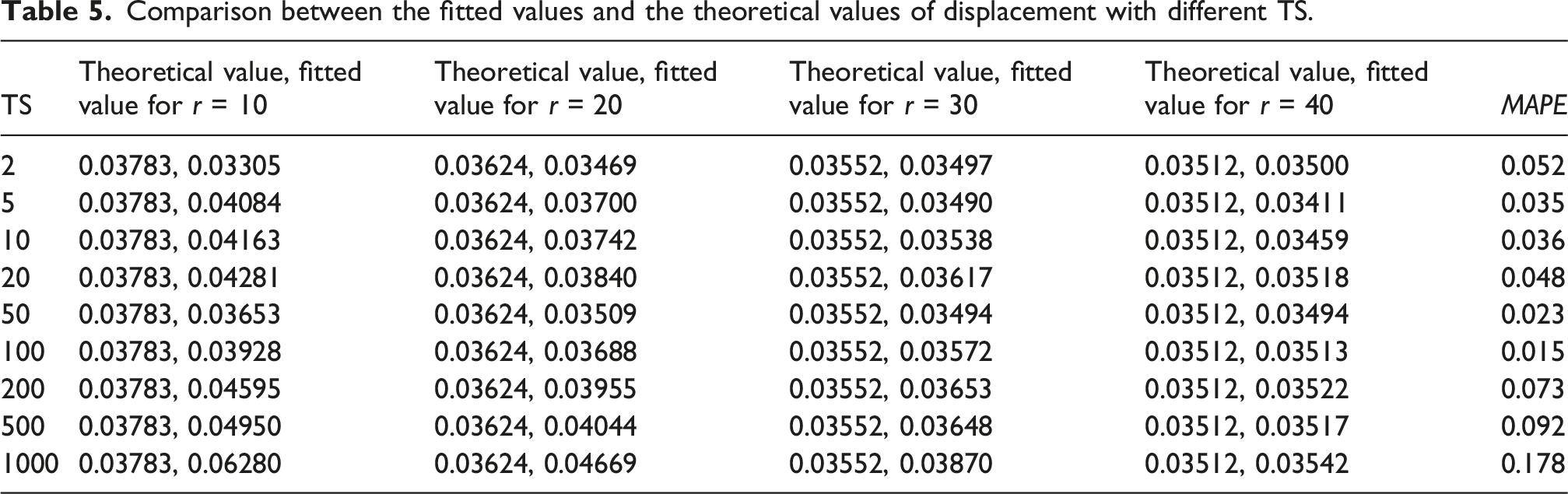
Comparison between the fitted values and the theoretical values of displacement with different TS.

TS	Theoretical value, fitted value for r = 10	Theoretical value, fitted value for r = 20	Theoretical value, fitted value for r = 30	Theoretical value, fitted value for r = 40	MAPE
2	0.03783, 0.03305	0.03624, 0.03469	0.03552, 0.03497	0.03512, 0.03500	0.052
5	0.03783, 0.04084	0.03624, 0.03700	0.03552, 0.03490	0.03512, 0.03411	0.035
10	0.03783, 0.04163	0.03624, 0.03742	0.03552, 0.03538	0.03512, 0.03459	0.036
20	0.03783, 0.04281	0.03624, 0.03840	0.03552, 0.03617	0.03512, 0.03518	0.048
50	0.03783, 0.03653	0.03624, 0.03509	0.03552, 0.03494	0.03512, 0.03494	0.023
100	0.03783, 0.03928	0.03624, 0.03688	0.03552, 0.03572	0.03512, 0.03513	0.015
200	0.03783, 0.04595	0.03624, 0.03955	0.03552, 0.03653	0.03512, 0.03522	0.073
500	0.03783, 0.04950	0.03624, 0.04044	0.03552, 0.03648	0.03512, 0.03517	0.092
1000	0.03783, 0.06280	0.03624, 0.04669	0.03552, 0.03870	0.03512, 0.03542	0.178

Figure 12.

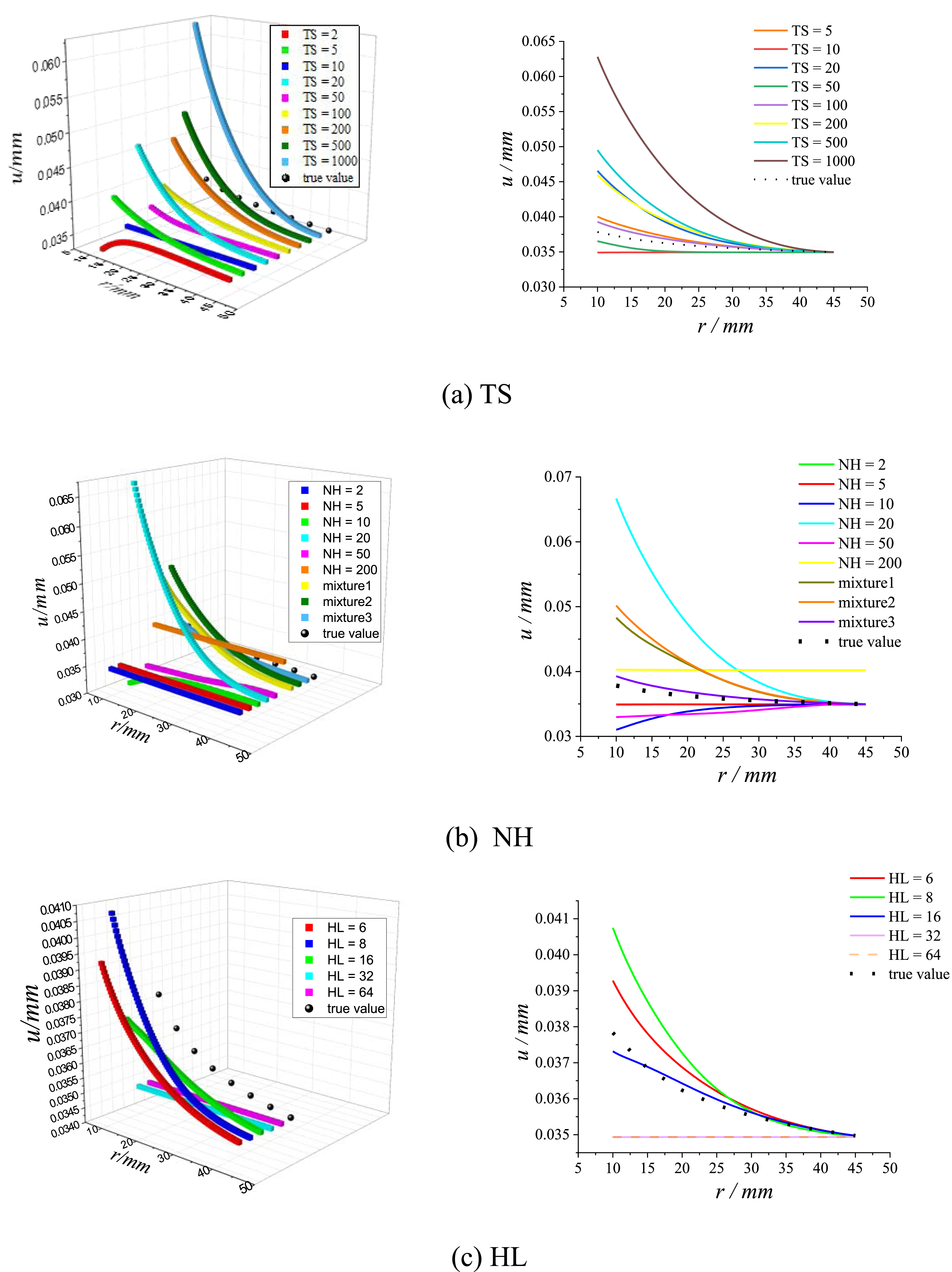
Comparison of the effects of different factors on the performance of neural networks (radial displacement). (a) TS; (b) NH; (c) HL.

In order to explore the effect of NH, the cracking process was modelled and radial displacement was fitted when W was 0.2 mm, HL was 6, and TS was 50. The NH was transformed, the gap between the radial displacement fitting effect and the theoretical value was compared, as shown in Table 6. Setting the number of neurons to increase and then decrease by hidden layer is more conducive to training, such as Mix 3, with a MAPE value of 0.015. This structure could make full use of the high-dimensional feature extraction ability of the early layers, and also improved the generalization ability of the model through the compression and simplification of the features in the later layers. It is also visually shown in Figure 12(b). So, the recommended number of neurons to train the hidden layer is the hybrid setting. The superior performance of the hybrid neuron configuration (Mix 3) can be attributed to its gradually expanding and then contracting structure. The wider middle layers provide sufficient nonlinear approximation capacity, while the narrower later layers help stabilize the output. This configuration is suitable for the radial displacement problem because it can capture the relatively steep variation near the inner boundary and the smoother variation near the outer boundary.

Table 6.

Comparison between the fitted values and the theoretical values of displacement with different NH.

NH	Theoretical value, fitted value for r = 10	Theoretical value, fitted value for r = 20	Theoretical value, fitted value for r = 30	Theoretical value, fitted value for r = 40	MAPE
2	0.03783, 0.03494	0.03624, 0.03494	0.03552, 0.03494	0.03512, 0.03494	0.035
5	0.03783, 0.03492	0.03624, 0.03493	0.03552, 0.03494	0.03512, 0.03494	0.036
10	0.03783, 0.03102	0.03624, 0.03384	0.03552, 0.03471	0.03512, 0.03491	0.080
20	0.03783, 0.06667	0.03624, 0.04734	0.03552, 0.03834	0.03512, 0.03534	0.187
50	0.03783, 0.03298	0.03624, 0.03343	0.03552, 0.03407	0.03512, 0.03491	0.070
100	0.03783, 10.6101	0.03624, 10.6101	0.03552, 10.6099	0.03512, 10.6098	0.997
200	0.03783, 0.04029	0.03624, 0.04024	0.03552, 0.04021	0.03512, 0.04020	0.101
500	0.03783, 9.6906	0.03624, 9.6906	0.03552, 9.6906	0.03512, 9.6906	0.996
1000	0.03783, 12.3376	0.03624, 12.3376	0.03552, 12.3376	0.03512, 12.3376	0.997
Mix 1	0.03783, 0.04829	0.03624, 0.04116	0.03552, 0.03684	0.03512, 0.03520	0.094
Mix 2	0.03783, 0.05017	0.03624, 0.04137	0.03552, 0.03691	0.03512, 0.03522	0.103
Mix 3	0.03783, 0.03928	0.03624, 0.03688	0.03552, 0.03572	0.03512, 0.03513	0.015

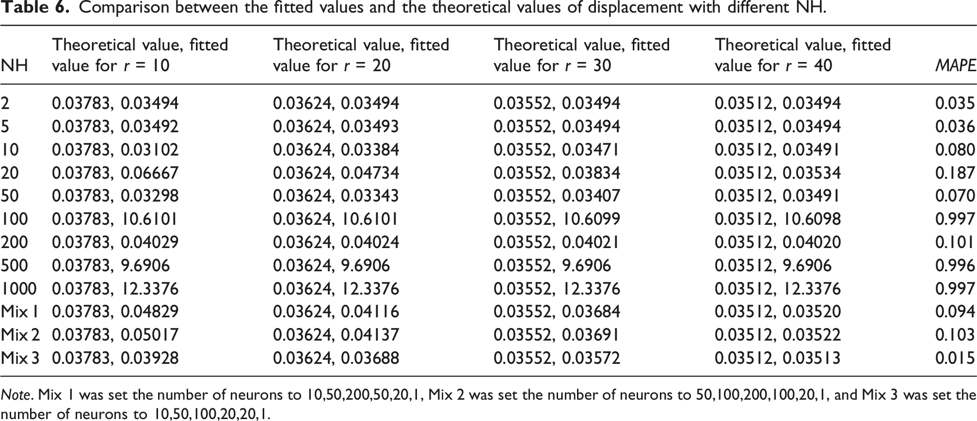
Note. Mix 1 was set the number of neurons to 10,50,200,50,20,1, Mix 2 was set the number of neurons to 50,100,200,100,20,1, and Mix 3 was set the number of neurons to 10,50,100,20,20,1.

In order to explore the effect of HL, the cracking process was modelled and radial displacement was fitted when W was 0.2 mm, TS was 50, the number of neurons in the first two layers of the hidden layer was 10,50, and the number of neurons in the last three layers was 20, 20, 1. The number of layers of the hidden layer with 100 neurons was changed, so as to choose the appropriate HL, as shown in Table 7. The increase in HL instead made the fitting effect of the neural network worse, resulting an overfitting phenomenon. It is also visually shown in Figure 12(c). For the efficiency of training, it is recommended that the interval of HL is 6–16.

Table 7.

Comparison between the fitted values and the theoretical values of displacement with different HL.

HL	Theoretical value, fitted value for r = 10	Theoretical value, fitted value for r = 20	Theoretical value, fitted value for r = 30	Theoretical value, fitted value for r = 40	MAPE
6	0.03783, 0.03928	0.03624, 0.03688	0.03552, 0.03572	0.03512, 0.03513	0.015
8	0.03783, 0.04075	0.03624, 0.03721	0.03552, 0.03563	0.03512, 0.03507	0.026
16	0.03783, 0.03732	0.03624, 0.03640	0.03552, 0.03561	0.03512, 0.03512	0.005
32	0.03783, 0.03493	0.03624, 0.03493	0.03552, 0.03493	0.03512, 0.03493	0.036
64	0.03783, 0.03493	0.03624, 0.03493	0.03552, 0.03493	0.03512, 0.03493	0.036

Physics-guided probabilistic deep learning-based modeling stability analysis

Stability analysis of circumferential stress fitting

Factors affecting the fitting effect of physics-guided probabilistic deep learning include HL, NH, and different weight calculation methods etc. In order to explore the effect of different ways, the cracking process was modelled when HL was 2 layers, NH was 50, the number of probability layers was 1, the TS was 50, and the number of epochs was 20,000, and W was 0.06 mm. The results of two different ways of weights calculation, reparameterization and Flipout are shown in Figure 13. The theoretical value of the circumferential stress at a radius of 10 mm is −4.79 MPa. It could be seen that the convergence speed of Flipout was not as fast as that of the reparameterization method. Flipout estimates the gradient by introducing a special kind of noise, whereas the reparameterization method directly transforms the stochastic variable into a deterministic one by means of the differentiable transformation. The noise introduced by Flipout may affect the model parameter updating to some extent, making the convergence speed slower.

Figure 13.

The effect of different weight calculation methods on the effectiveness of the fit. (a) Reparameterization; (b) Flipout.

In order to explore the effect of different HL, the cracking process was modelled when NH was 50, the number of probability layers was 1, the TS was 50, and the number of epochs was 20,000, the gradient was calculated by the reparameterization method, and W was 0.06 mm. The fitting effect of the networks with HL of 2, 10 and 50 layers was compared, respectively, as shown in Figure 14. The theoretical value of the circumferential stress at a radius of 10 mm is −4.79 MPa. From the figure, it could be seen that excessively increasing the HL could not increase the performance of the prediction, but rather decreased it. This show that adding HL can improve the expression ability of the model, but this improvement is bounded. When the complexity of the model exceeds a certain limit, further adding HL may not significantly improve the performance, but rather increase the computational cost and reduce the running efficiency of the code.

Figure 14.

The effect of HL on the effectiveness of the fit. (a) HL = 2; (b) HL = 10; (c) HL = 50.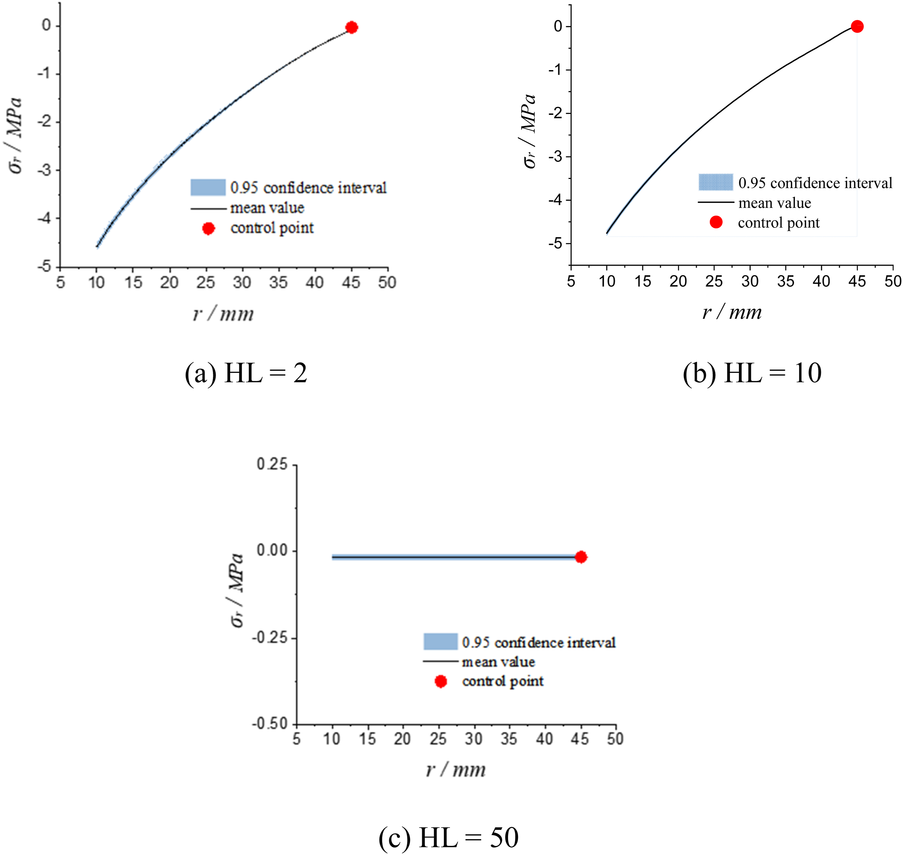

In order to explore the effect of different NH, the cracking process was modelled when HL was 2, the number of probability layers was 1, the TS was 50, and the number of epochs was 20,000, the gradient was calculated by the reparameterization method, and W was 0.06 mm. The fitting effect of the network was compared when the NH was 5, 50, and 300, as shown in Figure 15. When the NH was drastically reduced, the prediction was significantly distorted. It means that the number of parameters of the model decreases, resulting in insufficient capacity of the model to capture complex patterns in the data. Increasing the NH results in a significant increase in the uncertainty of the prediction, while the performance of the prediction is not significantly improved. Increasing the NH will make it easier to fit the noise in the training data, and thus the model’s prediction uncertainty will increase. At this point, the model has already reached the upper limit of its expressive capacity. Thus, continuing to increase the number of neurons will only lead to an increase in the model’s complexity, and will not improve the model’s prediction performance.

Figure 15.

The effect of NH on the effectiveness of the fit. (a) NH = 5; (b) NH = 50; (c) NH = 300.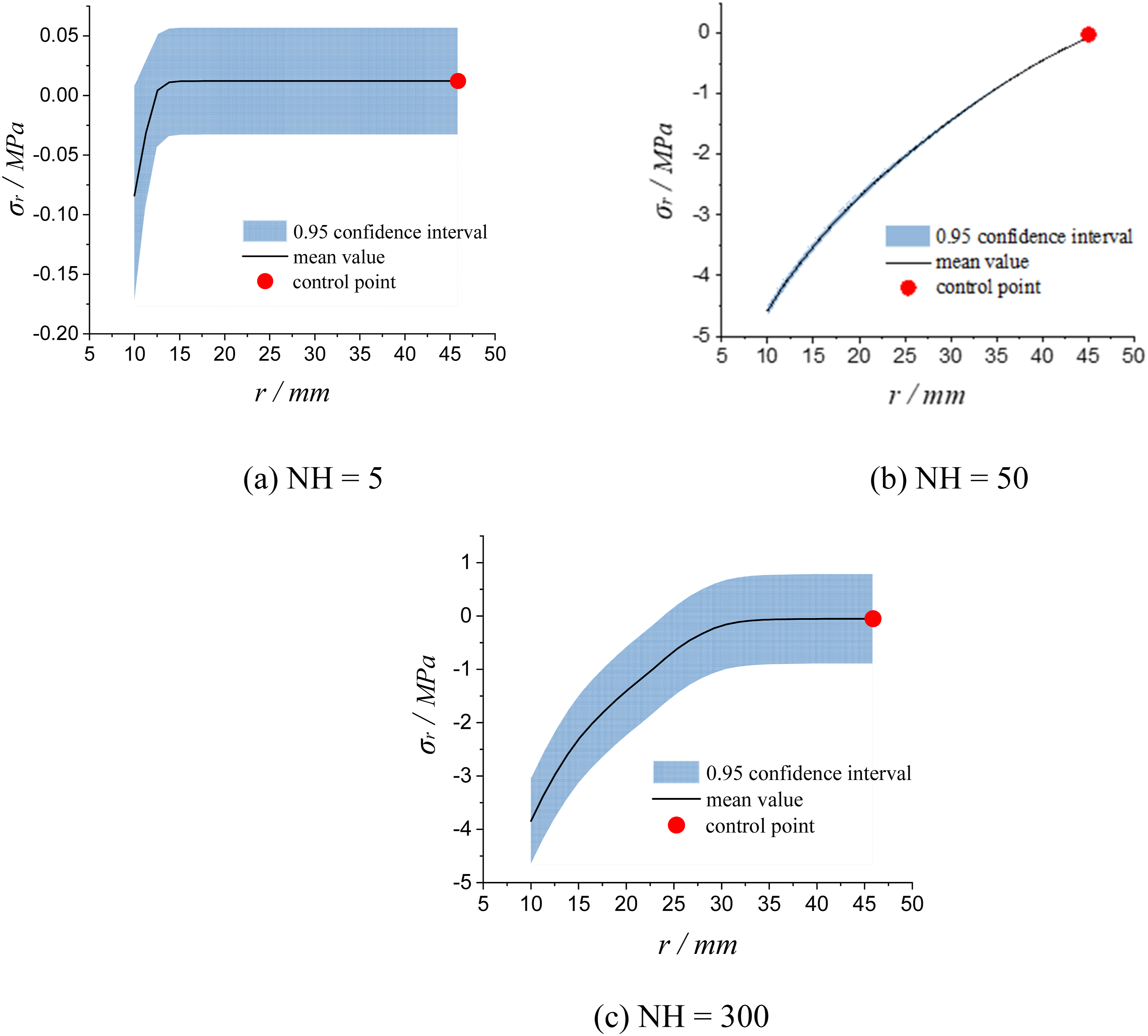

Stability analysis of radial displacement fitting

In order to explore the effect of different weight calculation methods, the cracking process was modelled when HL was 6, the number of probability layers was 1, the TS was 50, and the number of epochs was 20,000, the number of neurons in the hidden layer was set to 10,50,100,20,20,1, and W was 0.2 mm. The fit of two different weights, reparameterization and Flipout was compared, as shown in Figure 16. The uncertainty interval of Flipout was large, and the convergence speed was not as fast as that of the reparameterization method, which was the same as the results and reasons of the stress part. From a practical standpoint, the reparameterization method is recommended for this problem due to its faster convergence and narrower uncertainty intervals. The Flipout method, while theoretically providing more decorrelated gradient estimates within a mini-batch, introduces additional noise that slows convergence when the training set is small, as is the case here. For problems with larger datasets or mini-batch training, Flipout may offer advantages in gradient estimation efficiency.

Figure 16.

The effect of different weight calculation methods on the effectiveness of the fit. (a) Reparameterization; (b) Flipout.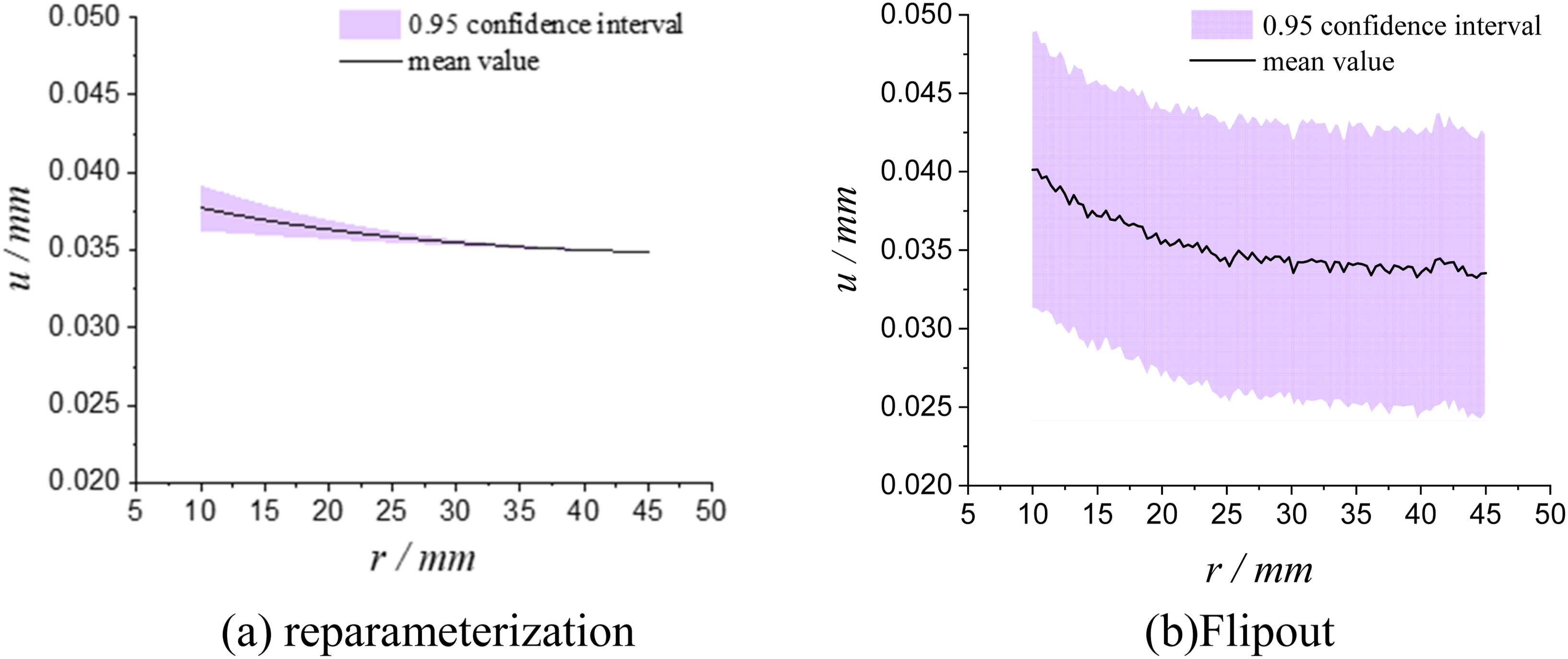

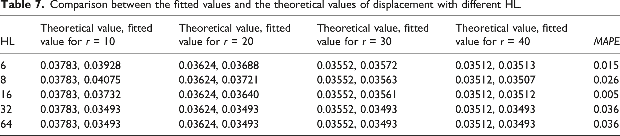
In order to explore the effect of different HL, the cracking process was modelled when HL was 6, the number of probability layers was 1, the TS was 50, and the number of epochs was 20,000, the weights were calculated by the reparameterization method, the number of neurons of the first two layers is 10,50, the number of neurons of the last three layers is 20, 20, 1, the number of neurons in the middle hidden layers is 100, and W was 0.2 mm. The number of layers of hidden layers with 100 neurons was transformed, as shown in Figure 17. The theoretical value of displacement is 0.03,783 mm for the radius of 10 mm and 0.03,497 mm for the radius of 45 mm. The addition of the hidden layer did not significantly increase the performance of the prediction, but rather made the code run slower, which was the same result and reason as in the stress section.

Figure 17.

The effect of HL on the effectiveness of the fit. (a) HL = 6; (b) HL = 8; (c) HL = 16; (d) HL = 32.

In order to explore the effect of different number of probability layers, the cracking process was modelled when HL was 6, the number of probability layers was 1, the TS was 50, and the number of epochs was 20,000, the weights were calculated by the reparameterization method, the number of neurons in the six hidden layers was set to 10, 50, 100, 20, 20, 1, and W was 0.2 mm. The fitting effects of the penultimate layer set as deterministic and probabilistic network layers respectively were compared respectively in Figure 18. Increasing the number of probabilistic layers increased the uncertainty of the predictions and did not increase the performance of the predictions, instead it made the code run slower. This indicates that as the number of probability layers increases, the randomness introduced in the model accumulates and the uncertainty increases. Meanwhile, the introduction of probabilistic layers usually increases the computational complexity of the model, thus increasing the training time.

Figure 18.

The effect of the number of probability layer on the effectiveness of the fit. (a) The number of probability layer layers is 1; (b) The number of probability layer layers is 2.

It should be noted that the recommended parameter ranges (Table 8) are derived from the specific case study presented in this paper. Some of the observed trends are consistent with general neural network behavior and may provide useful reference for similar physics-informed modeling tasks. For example, model performance degrades when neurons are too few or too many, and increasing hidden layers beyond a certain depth yield diminishing returns. However, the specific numerical ranges recommended here are influenced by the particular governing equations, boundary conditions, and computational domain of this study. They may therefore require adjustment when applied to other corrosion scenarios, material properties, or structural configurations.

Table 8.

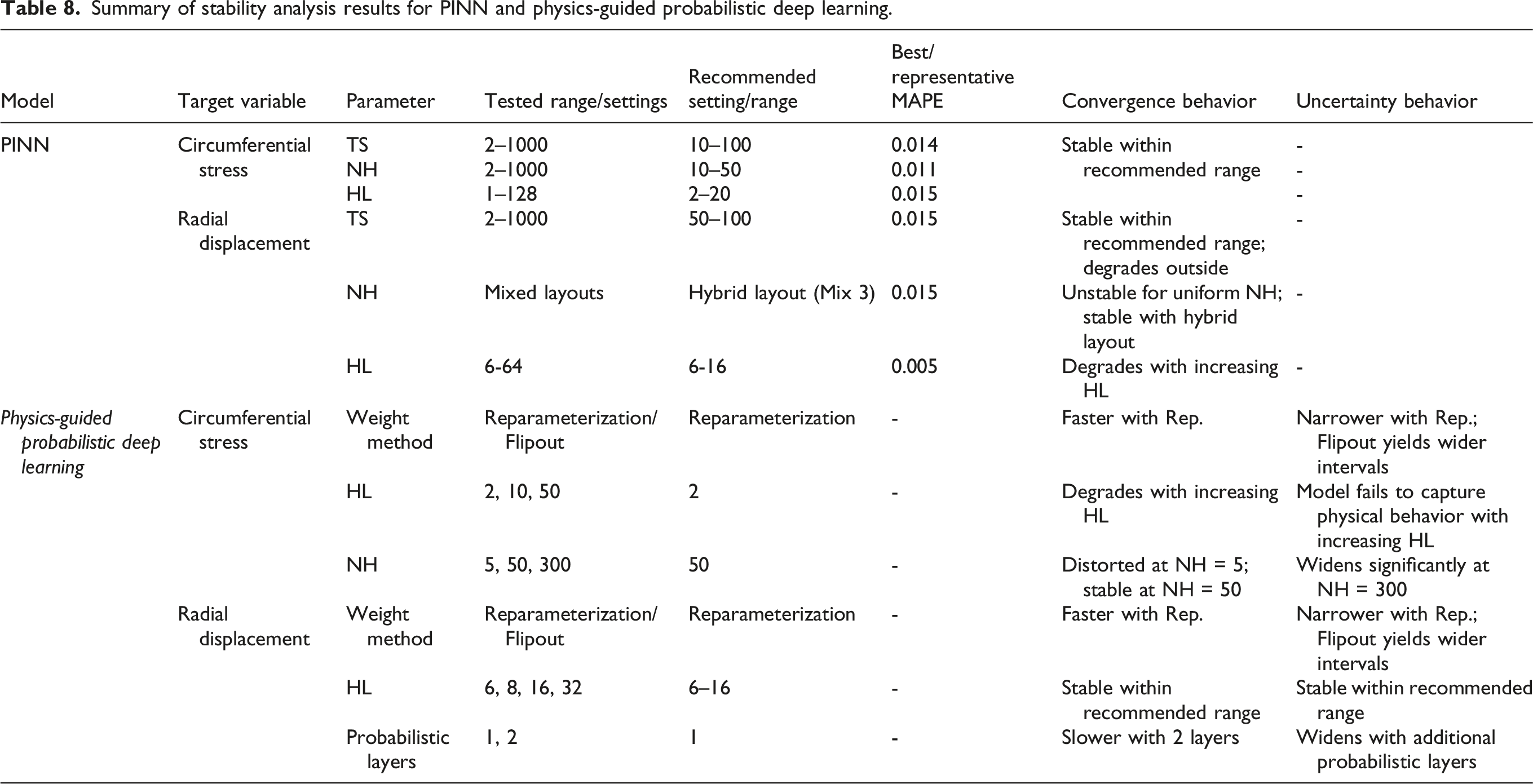
Summary of stability analysis results for PINN and physics-guided probabilistic deep learning.

Model	Target variable	Parameter	Tested range/settings	Recommended setting/range	Best/representative MAPE	Convergence behavior	Uncertainty behavior
PINN	Circumferential stress	TS	2–1000	10–100	0.014	Stable within recommended range	-
		NH	2–1000	10–50	0.011		-
		HL	1–128	2–20	0.015		-
	Radial displacement	TS	2–1000	50–100	0.015	Stable within recommended range; degrades outside	-
		NH	Mixed layouts	Hybrid layout (Mix 3)	0.015	Unstable for uniform NH; stable with hybrid layout	-
		HL	6-64	6-16	0.005	Degrades with increasing HL	-
Physics-guided probabilistic deep learning	Circumferential stress	Weight method	Reparameterization/Flipout	Reparameterization	-	Faster with Rep.	Narrower with Rep.; Flipout yields wider intervals
		HL	2, 10, 50	2	-	Degrades with increasing HL	Model fails to capture physical behavior with increasing HL
		NH	5, 50, 300	50	-	Distorted at NH = 5; stable at NH = 50	Widens significantly at NH = 300
	Radial displacement	Weight method	Reparameterization/Flipout	Reparameterization	-	Faster with Rep.	Narrower with Rep.; Flipout yields wider intervals
		HL	6, 8, 16, 32	6–16	-	Stable within recommended range	Stable within recommended range
		Probabilistic layers	1, 2	1	-	Slower with 2 layers	Widens with additional probabilistic layers

Conclusions

In the study, focusing on the cracking model of corroded steel-bar concrete at the stage of complete cracking, damage theory was used for corrosion cracking, and diffuse crack theory was used for the crack distribution case. Steel-bar concrete was simplified into an anisotropic thick-walled cylinder, and the cracking process was modeled with physics-guided probabilistic deep learning. The results of the study can be summarized as follows:

(1) Focusing on the complete cracking stage, for solving the differential equations triggered by the change of circumferential stress and displacement with radius, physics-guided probabilistic deep learning was applied. The MAPE values of the corrosion expansion force and the radial displacement of the steel-bar concrete contact surface were 0.58% and 4.6%, respectively.

(2) This provided a new idea for the modeling process of the cracking stage of corroded steel-bar concrete and the subsequent problem solving. It also achieved a quantitative analysis of the uncertainty of the output results, and increased solution performance and generalization ability.

(3) Modeling stability analysis of cracking in corroded reinforced concrete for PINN was achieved. In the fitting process of stress, the optimal interval of the TS was 10-100, the optimal interval of the NH was 10–50, and the optimal interval of the HL was 2–20; in the fitting process of displacement, the optimal interval of the TS was 50–100, and the optimal effect was achieved by setting the NH to increase firstly and then decrease, and the optimal interval of the HL was 6–16.

(4) Modeling stability analysis of cracking in corroded reinforced concrete for physics-guided probabilistic deep learning was achieved. The TS, the NH, and the HL should likewise not be too large or too small; The convergence speed of the weight calculation method Flipout was not as fast as that of the reparameterization method; Increasing the number of probabilistic layer layers increased the uncertainty of prediction, and did not increase the performance of prediction.

The primary novelty of this study lies in the integration of Bayesian inference into the PINN framework, enabling the model to move beyond deterministic predictions and produce probabilistic outputs with quantified uncertainty. This physics-guided probabilistic deep learning approach bridges the gap between physics-based modeling and uncertainty-aware machine learning in the context of corrosion-induced cracking in reinforced concrete. From a practical engineering perspective, the proposed framework offers a computationally efficient alternative to conventional numerical methods for assessing the cracking process in corroded reinforced concrete structures. The quantified uncertainty bounds on the predicted corrosion expansion force and radial displacement can directly support structural inspection decision-making, remaining service life estimation, and risk-based maintenance planning. This is particularly valuable in practical scenarios where experimental data are scarce or material parameters are subject to variability.

Nevertheless, several limitations should be acknowledged. The framework is validated against analytical solutions rather than independent experimental data, the uniform corrosion assumption may not capture non-uniform corrosion patterns in chloride-dominated environments, and the simplified thick-walled cylinder geometry may not represent complex structural configurations in practice. Future research could address these limitations by incorporating experimental validation using published corrosion cracking datasets, extending the model to non-uniform corrosion and two- or three-dimensional geometries, and investigating the transferability of the recommended hyperparameter ranges to other structural configurations.

Footnotes

Acknowledgments

The authors gratefully acknowledge the support from the Deep Earth Probe and Mineral Resources Exploration-National Science and Technology Major Project (Grant No. 2024ZD1004103), the Special Funding Support for Taishan Scholars Project (Grant No. tsqn202408036) and the Shandong Provincial Natural Science Foundation (Grant No. ZR2025QC1114).

ORCID iDs

Yang Zhang

Li Li

Funding

The authors disclosed receipt of the following financial support for the research, authorship, and/or publication of this article: This study is supported by The Deep Earth Probe and Mineral Resources Exploration-National Science and Technology Major Project; 2024ZD1004103. The Special Funding Support for Taishan Scholars Project; tsqn202408036. The Shandong Provincial Natural Science Foundation; ZR2025QC1114.

Declaration of conflicting interests

The authors declared no potential conflicts of interest with respect to the research, authorship, and/or publication of this article.

References

Ananthi

GBG

(2022) Plastic Hinge length mechanism of steel-fiber-reinforced concrete slab under repeated loading. Journal of Composites Science 6(6): 164.

Basora

Arthur

Arias Chao

, et al. (2025) A benchmark on uncertainty quantification for deep learning prognostics. Reliability Engineering & System Safety 253: 110513. https://doi.org/10.1016/j.ress.2024.110513

Behera

Kumar

AVSP

Nayak

(2024) Analyzing the performance of geometric mean optimization-based artificial neural networks for cryptocurrency forecasting. International Journal of Information Technology 17: 2511.

Belov

Armstrong

(2011) Distributions of the Kullback--Leibler divergence with applications. British Journal of Mathematical and Statistical Psychology 64(2): 291-309. https://doi.org/10.1348/000711010X522227

Blundell

Cornebise

Kavukcuoglu

, et al. (2015) Weight Uncertainty in Neural Networks. Proceedings of the 32nd International Conference on Machine Learning 37: 1613-1622. Available at: https://arxiv.org/abs/1505.05424

Bonfanti

Santana

Ellero

, et al. (2023) On the generalization of PINNs outside the training domain and the hyperparameters influencing it. Neural Computing and Applications 36: 22677–22696.

Chang

L-Z

Jonathan

Karin

(2024) 3D modelling of the interaction between bending and corrosion-induced cracks in reinforced concrete beams. Construction and Building Materials 411: 134272. https://doi.org/10.1016/j.conbuildmat.2023.134272

Chen

Xiao

(2012) Analytical solutions for corrosion induced cohesive concrete cracking. Journal of Applied Mathematics 2012: 1–25. https://doi.org/10.1155/2012/769132

Chen

Liu

Sun

(2021) Physics-informed learning of governing equations from scarce data. Nature Commununications 12: 6136. https://doi.org/10.1038/s41467-021-26434-1

10.

Gao

Sun

Jian-Xun

(2020) PhyGeoNet: physics-Informed geometry-adaptive convolutional neural networks for solving parameterized steady-state PDEs on irregular domain. Journal of Computational Physics 428: 110079.

11.

Gelman

Carlin John

Stern Hal

, et al. (2013) Bayesian Data Analysis. CRC Press.

12.

Graves

(2011) Practical variational inference for neural networks. Advances in Neural Information Processing Systems. Curran Associates, Inc, 24, 2348–2356.

13.

Guo

(2014) Principles of Reinforced Concrete. Tsinghua University Press.

14.

Jagtap

Kawaguchi

Em Karniadakis

(2020) Adaptive activation functions accelerate convergence in deep and physics-informed neural networks. Journal of Computational Physics 404: 109136. https://doi.org/10.1016/j.jcp.2019.109136

15.

Kingma

Jimmy

(2015) Adam: a method for stochastic optimization. Proceedings of the 3rd International Conference on Learning Representations. Available at: https://arxiv.org/abs/1412.6980

16.

Kingma

Welling

(2013) Auto-encoding variational bayes. arXiv preprint arXiv:1312.6114. Available at: https://arxiv.org/abs/1312.6114

17.

Lagaris

Likas

Fotiadis

(1998) Artificial neural networks for solving ordinary and partial differential equations. IEEE Transactions on Neural Networks 9(5): 987–1000. https://doi.org/10.1109/72.712178

18.

Langseth

Portinale

(2007) Bayesian networks in reliability. Reliability Engineering & System Safety 92(1): 92–108. https://doi.org/10.1016/j.ress.2005.11.037

19.

Lee

Kwon

(2023) Dynamic Bayesian network model for comprehensive risk analysis of fatigue-critical structural details. Reliability Engineering & System Safety 229: 108834. https://doi.org/10.1016/j.ress.2022.108834

20.

Melchers

Zheng

(2006) Analytical model for corrosion-induced crack width in reinforced concrete structures. ACI Structural Journal 103: 479–487.

21.

Yihang

Yang

, et al. (2024) Bond strength between recycled aggregate concrete and rebar: interpretable machine learning modeling approach for performance estimation and engineering design. Materials Today Communications 39: 108945. https://doi.org/10.1016/j.mtcomm.2024.108945

22.

Liang

Wang

(2020) Prediction of corrosion-induced cracking of concrete cover: a critical review for thick-walled cylinder models. Ocean Engineering 213: 107688. https://doi.org/10.1016/j.oceaneng.2020.107688

23.

Liu

Sun

Liu

, et al. (2025) Quantitative risk assessment for connected automated vehicles: integrating improved STPA-SafeSec and Bayesian network. Reliability Engineering & System Safety 253: 110528. https://doi.org/10.1016/j.ress.2024.110528

24.

Long

Zhang

Zhou

(2008) A comparative study for concrete fracture analysis using smeared and discrete-crack model. Engineering Mechanics 25(3): 80–84.

25.

Jin

Liu

(2011) Reinforcement corrosion-induced cover cracking and its time prediction for reinforced concrete structures. Corrosion Science 53(4): 1337–1347. https://doi.org/10.1016/j.corsci.2010.12.026

26.

Mazars

Pijaudier

(1989) Continuum damage theory - application to concrete. Journal of Engineering Mechanics 115(2): 223–446.

27.

Meng

Zhen

Zhang

, et al. (2020) PPINN: parareal physics-informed neural network for time-dependent PDEs. Computer Methods in Applied Mechanics and Engineering 370: 113250. https://doi.org/10.1016/j.cma.2020.113250

28.

Meng

Mengqian

Kong

, et al. (2024) Risk analysis of lithium-ion battery accidents based on physics-informed data-driven Bayesian networks. Reliability Engineering & System Safety 251: 110294. https://doi.org/10.1016/j.ress.2024.110294

29.

Miele

Karve

Mahadevan

(2023) Multi-fidelity physics-informed machine learning for probabilistic damage diagnosis. Reliability Engineering & System Safety 235: 109243. https://doi.org/10.1016/j.ress.2023.109243

30.

Monaco

Apiletti

(2023) Training physics-informed neural networks: one learning to rule them all? Results in Engineering 18: 101023. https://doi.org/10.1016/j.rineng.2023.101023

31.

Nabian

Gladstone

Meidani

(2021) Efficient training of physics‐informed neural networks via importance sampling. Computer-Aided Civil and Infrastructure Engineering 36: 962–977. https://doi.org/10.1111/mice.12685

32.

Pan

Sun

, et al. (2024) Probabilistic remaining useful life prediction without lifetime labels: a Bayesian deep learning and stochastic process fusion method. Reliability Engineering & System Safety 250: 110313. https://doi.org/10.1016/j.ress.2024.110313

33.

Pantazopoulou

Papoulia

(2001) Modeling cover cracking due to reinforcement corrosion in RC structures. Journal of Engineering Mechanics 127(4): 342–351. https://doi.org/10.1061/(asce)0733-9399(2001)127:4(342)

34.

Philip

Baby

Soorya

, et al. (2023) A comparative study on crack detection in concrete walls using transfer learning techniques. Journal of Composites Science 7(4): 169. https://doi.org/10.3390/jcs7040169

35.

Qin

Kaewunruen

(2024) Machine learning and traditional approaches in shear reliability of steel fiber reinforced concrete beams. Reliability Engineering & System Safety 251: 110339. https://doi.org/10.1016/j.ress.2024.110339

36.

Raissi

Karniadakis

(2018) Hidden physics models: machine learning of nonlinear partial differential equations. Journal of Computational Physics 357: 125–141. https://doi.org/10.1016/j.jcp.2017.11.039

37.

Raissi

Perdikaris

Karniadakis

(2019) Physics-informed neural networks: a deep learning framework for solving forward and inverse problems involving nonlinear partial differential equations. Journal of Computational Physics 378: 686–707. https://doi.org/10.1016/j.jcp.2018.10.045

38.

Rao

Sun

Liu

(2020) Physics-informed deep learning for incompressible laminar flows. Theoretical and Applied Mechanics Letters 10(3): 207–212. https://doi.org/10.1016/j.taml.2020.01.039

39.

Reis

de Azevedo

Christoforo

, et al. (2023) Bonding of steel bars in concrete: a systematic review of the literature. Structures 49: 508–519. https://doi.org/10.1016/j.istruc.2023.01.141

40.

Šavija

Luković

Pacheco

, et al. (2013) Cracking of the concrete cover due to reinforcement corrosion: a two-dimensional lattice model study. Construction and Building Materials 44: 626–638. https://doi.org/10.1016/j.conbuildmat.2013.03.063

41.

Scneidereit

Breuss

(2022) Computational characteristics of feedforward neural networks for solving a stiff differential equation. Neural Computing & Applications 34(10): 7975–7989.

42.

RKL

Zhang

(2015) A double-cylinder model incorporating confinement effects for the analysis of corrosion-caused cover cracking in reinforced concrete structures. Corrosion Science 99: 205–218. https://doi.org/10.1016/j.corsci.2015.07.009

43.

Uddin

Ganga

Asthana

, et al. (2023) Wavelets based physics informed neural networks to solve non-linear differential equations. Science Reports 13: 2882. https://doi.org/10.1038/s41598-023-29806-3

44.

Wan

(2019) Bayesian multi-task learning methodology for reconstruction of structural health monitoring data. Structural Health Monitoring 18(4): 1282–1309. https://doi.org/10.1177/1475921718794953

45.

Wan

Zhu

Luo

, et al. (2025) Unsupervised deep learning approach for structural anomaly detection using probabilistic features. Structural Health Monitoring 24(1): 247–264. https://doi.org/10.1177/14759217241226804

46.

Wang

Jin

, et al. (2014) Cover cracking model in reinforced concrete structures subject to rebar corrosion. Journal of Zhejiang University - Science A 15: 496–507. https://doi.org/10.1631/jzus.a1300393

47.

Wang

Bao

Ueda

(2016) Prediction of mass transport in cracked-unsaturated concrete by mesoscale lattice model. Ocean Engineering 127: 144–157. https://doi.org/10.1016/j.oceaneng.2016.09.044

48.

Wang

Zhang

Haibin

, et al. (2020) Deep learning of subsurface flow via theory-guided neural network. Journal of Hydrology 584: 124700. https://doi.org/10.1016/j.jhydrol.2020.124700

49.

Wang

, et al. (2024) Machine learning to estimate the bond strength of the corroded steel bar-concrete. Structural Concrete 25: 696–715. https://doi.org/10.1002/suco.202300401

50.

Wen

Vicol

, et al. (2018) Flipout: efficient pseudo-independent weight perturbations on mini-batches. Proceedings of the 6th International Conference on Learning Representations. Available at: https://arxiv.org/abs/1803.04386

51.

(2013) Two-Stage Model and Crack Development in Reinforced Concrete Structures with Rebar Corrosion. Zhejiang University.

52.

Xiao

Yang

Chen

, et al. (2016) Analytical solutions for cohesive concrete cracking due to non-uniform corrosion of the steel reinforcements. In: Life-Cycle of Engineering Systems: Emphasis on Sustainable Civil Infrastructure. CRC Press, pp. 373–378.

53.

Yang

Meng

Karniadakis

(2021) B-PINNs: bayesian physics-informed neural networks for forward and inverse PDE problems with noisy data. Journal of Computational Physics 425: 109913. https://doi.org/10.1016/j.jcp.2020.109913

54.

Bin

Wencheng

(2025) Resilience evaluation of train control on-board system considering component failure correlations: based on apriori-multi layer-copula bayesian network model. Reliability Engineering & System Safety 253: 110514. https://doi.org/10.1016/j.ress.2024.110514

55.

Zhang

Yuen

(2022) Physically guided deep learning solver for time-dependent Fokker-Planck equation. International Journal of Non-linear Mechanics 147: 104202. https://doi.org/10.1016/j.ijnonlinmec.2022.104202

56.

Zhang

Tang

, et al. (2017) Corrosion induced stress field and cracking time of reinforced concrete with initial defects: analytical modeling and experimental investigation. Corrosion Science 120: 158–170. https://doi.org/10.1016/j.corsci.2017.01.012

57.

Zhang

Yi-Qing

Jia

, et al. (2023a) Identification of concrete surface damage based on probabilistic deep learning of images. Automation in Construction 156: 105141. https://doi.org/10.1016/j.autcon.2023.105141

58.

Zhang

Run-Fa

Ka-Veng

(2023b) Neural network-based analytical solver for Fokker-Planck equation. Engineering Applications of Artificial Intelligence 125: 106721. https://doi.org/10.1016/j.engappai.2023.106721

59.

Zhang

Dang

Wang

, et al. (2024a) Damage identification for railway tracks using ultrasound guided wave and hybrid probabilistic deep learning. Construction and Building Materials 418: 135466. https://doi.org/10.1016/j.conbuildmat.2024.135466

60.

Zhang

Zou

Ellen

, et al. (2024b) Discovering a reaction-diffusion model for Alzheimer’s disease by combining PINNs with symbolic regression. Computer Methods in Applied Mechanics and Engineering 419: 116647. https://doi.org/10.1016/j.cma.2023.116647

61.

Zhao

Jin

(2006) Modeling the amount of steel corrosion at the cracking of concrete cover. Advances in Structural Engineering 9(5): 687–696. https://doi.org/10.1260/136943306778827556

62.

Zhao

Jiang

Jin

(2011) Damage analysis and cracking model of reinforced concrete structures with rebar corrosion. Corrosion Science 53(10): 3388–3397. https://doi.org/10.1016/j.corsci.2011.06.018

63.

Zhao

Dong

, et al. (2016) Corrosion-induced concrete cracking model considering corrosion product-filled paste at the concrete/steel interface. Construction and Building Materials 116: 273–280. https://doi.org/10.1016/j.conbuildmat.2016.04.097

64.

Zhao

Wang

Dong

(2021) Prediction of corrosion-induced concrete cracking under external loading and stirrup constraint. Construction and Building Materials 266: 121053. https://doi.org/10.1016/j.conbuildmat.2020.121053