Sweep frequency remote field eddy current testing for thickness estimation of small diameter ferritic steel tube

Abstract

This paper presents the 2D axi-symmetric finite element modeling and experimental studies carried out towards estimation of thickness of ferritic steel tube using sweep frequency remote field eddy current (RFEC) technique. The inductive reactance component of the impedance of the RFEC receiver coil as a function of frequency was predicted and analyzed to arrive at a unique value of frequency called as the peak frequency. A perfect linear relationship was observed between this peak frequency and thickness of the tube. The peak frequency variation for thickness reduction in the tube arising due to extended and localized corrosion type of degradation was analyzed in detail and results are presented. An attempt was also made to size the remaining wall thickness of the tubes from the peak frequency parameter. Experimental measurements were also found to be in good agreement with the model predictions. Studies are promising for accurate and absolute thickness estimation of ferritic steel tubes using sweep frequency RFEC technique.

Keywords

remote field eddy current sweep frequency finite element modeling ferromagnetic tubes nonlinear magnetic permeability

Introduction

Remote field eddy current (RFEC) technique is used for in-service inspection of ferromagnetic pipes and tubes.^1,2 This technique is efficient in detecting localized flaws in ferromagnetic tubes with better sensitivity than the conventional eddy current technique performed at the same frequency.³ However, in addition to detection of defects, it is often desired to estimate the thickness of the tubes, especially when large extended or uniform corrosion is expected. Modified 9Cr-1Mo steam generator tube of fast breeder reactors is one such component wherein the tubes are subjected to high pressure supersaturated steam in the ID side and high temperature sodium on the OD side. The minimum acceptable thickness of these tubes is 1.85 mm. Periodic in-service inspection (ISI) of these tubes is planned using RFEC technique. Estimation of the remaining wall thickness of the tubes is envisaged during ISI, in addition to detection of localized defects.

The phase change of the receiver coil voltage measured in the RFEC technique linearly varies with the wall thickness. This feature of the technique can be exploited to estimate the wall thickness of the tubes based on a calibration curve approach. However, it is only a relative measurement and prone to errors. Sweep frequency technique is promising in this context for absolute measurement of thickness.⁴ In sweep frequency technique the frequency of excitation is varied to measure the frequency dependent impedance change of the coil. Especially the quadrature component of the impedance, which is zero at extreme frequencies i.e., f = 0 and f=∞.⁵ Hence at some intermediate frequency, it should have a maximum value. This characteristic frequency called the peak frequency is proportional to the thickness of the tube. Thus, measurement of the peak frequency by sweeping the excitation frequency in a specific range would yield an absolute measurement of thickness as there exists a unique frequency for each thickness.

This paper presents for the first time the finite element model based studies carried out to understand the variation of the peak frequency with extended and localized wall thickness in small diameter (OD 17.2 mm, nominal thickness 2.3 mm) modified 9Cr-1Mo SG tubes. It also presents the details of development of a sweep frequency RFEC instrument and experimental determination of thickness in this ferritic steel tube.

Finite element modeling

A 2D axisymmetric finite element model was developed to investigate the variations in the excitation frequency as a function of thickness of the steam generator tubes. In this study, Finite Element Method Magnetics (FEMM) software was used to solve the governing partial differential equation of eddy current behavior in conducting and magnetic material as given below:

\nabla \times [\frac{1}{μ (H)} \nabla \times A] = - j σ ω A - σ \nabla V + J_{s}

(1)

where A is vector potential, V is scalar potential, J_s is source current density, ω = 2πf, in which f is excitation frequency, σ is electrical conductivity and µ is the magnetic permeability of the material. FEMM is an open-source finite element software for electromagnetics (static and quasi-static). In ferromagnetic materials, the magnetic permeability is a nonlinear function of the applied magnetic field (H). FEMM software handles this type of nonlinear magnetic material property through the concept of complex effective permeability. The formalism is based on an effective BH curve as reported in.^6,7 For this case, the virgin BH hysteresis curve of the material (shown in Figure 1) is given as input to the model so that the solver ensures nonlinear BH relation in the solution domain especially when the excitation currents are higher enough for nonlinear magnetic effects to be present. However, in practical cases very low excitation currents are used.

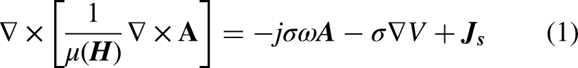
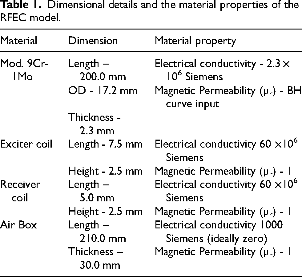
Figure 2 (a) shows the 2D axi-symmetric geometric model of the RFEC problem with the optimized finite element mesh. The geometry consists of a modified 9Cr-1Mo tube, exciter and receiver coils kept at an axial separation of 35 mm (optimized based on finite element modeling and experimental pull-out test). The dimensions and the material properties used in the model are given in Table 1. A rectangular air box surround the tube-coil geometry as shown in the figure. Asymptotic boundary condition was defined at the outer boundary of the air box. This boundary condition reduces the effective size of the outer boundary so that higher number of mesh nodes in the outer air box could be reduced leading to quicker solution time.⁸

Figure 1.

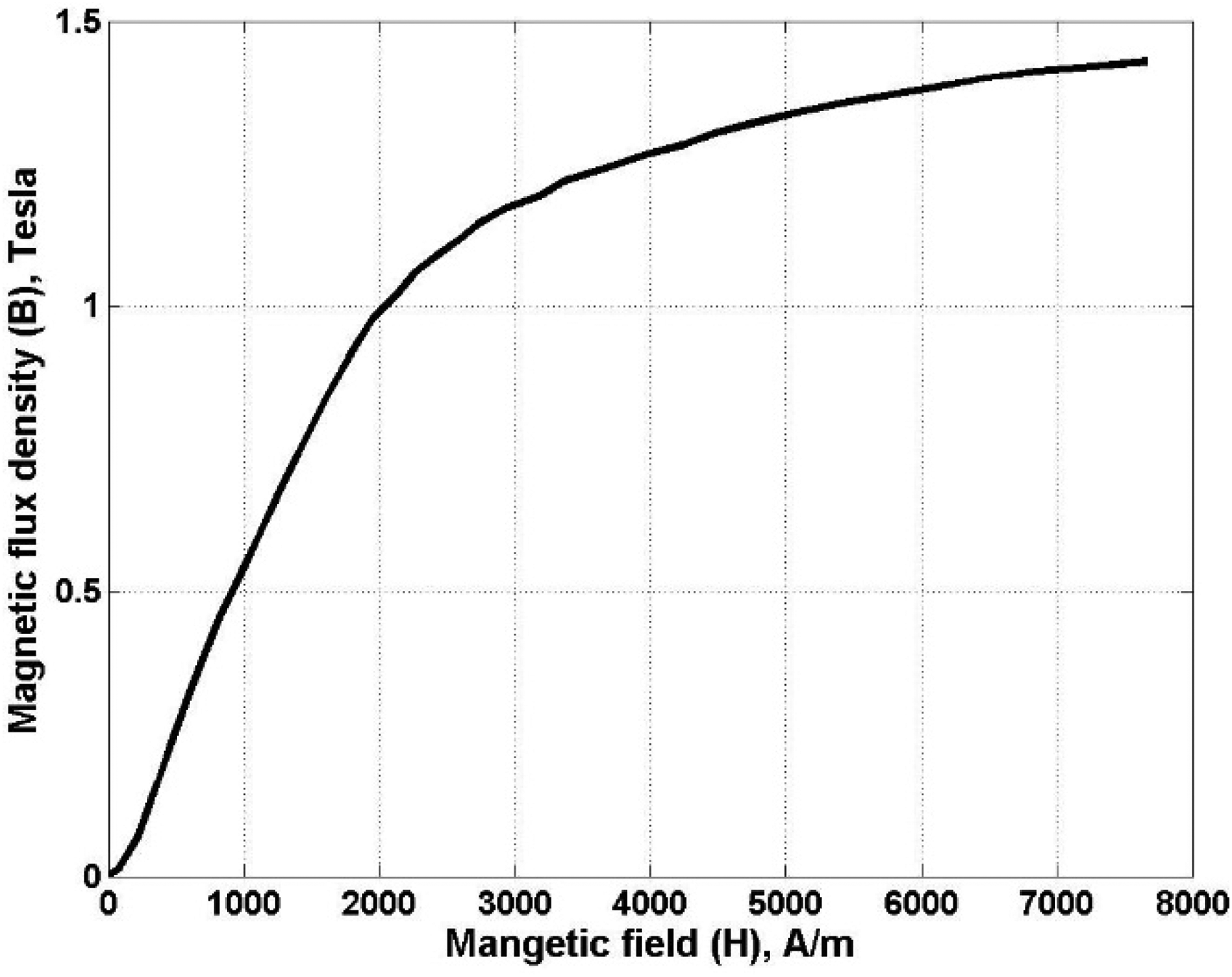
Measured BH curve of modified 9Cr-1Mo steel.

Figure 2.

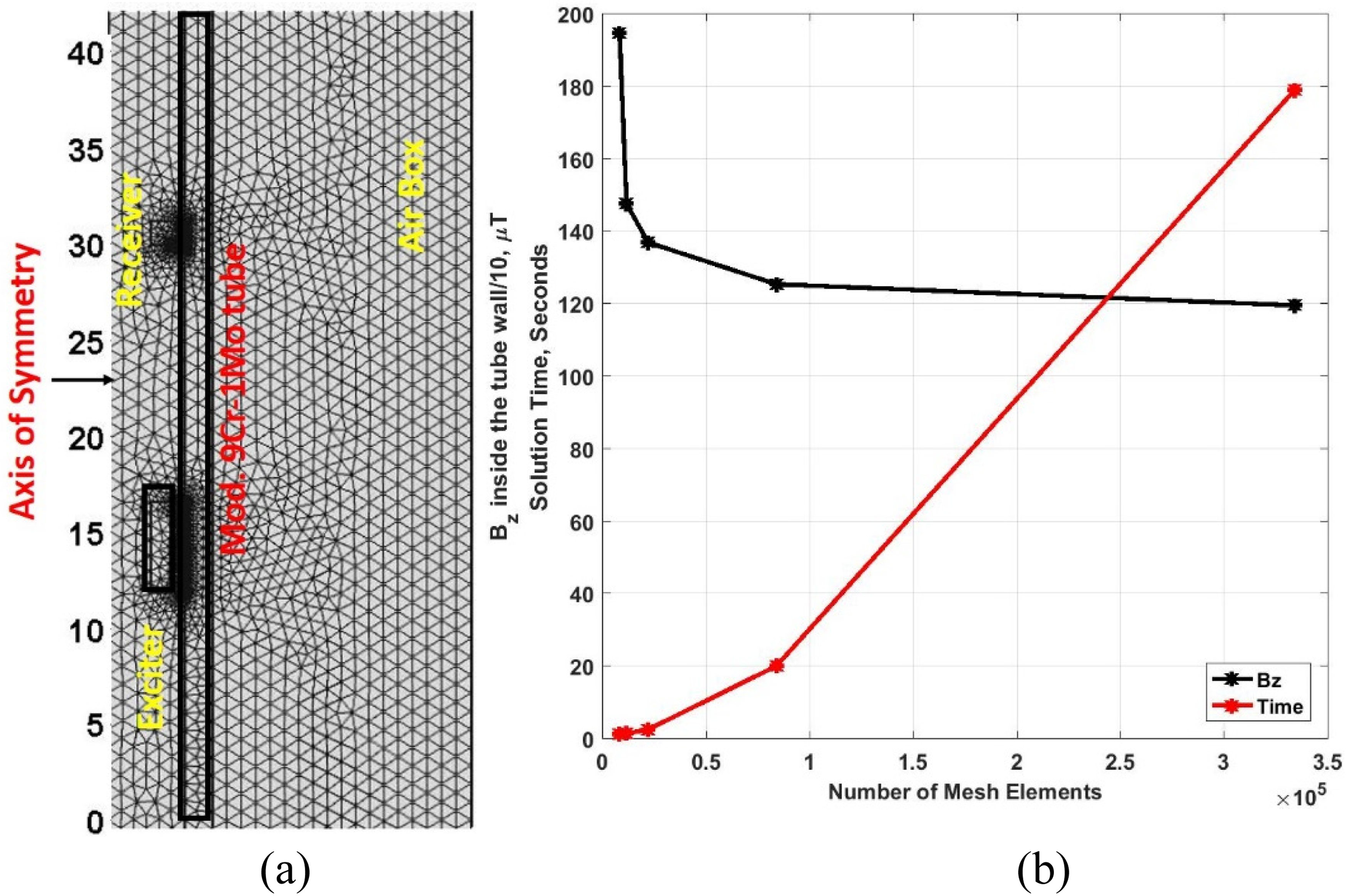
Geometry and meshing of the 2D axi-symmetric RFEC finite element model.

Table 1.

Dimensional details and the material properties of the RFEC model.

Material	Dimension	Material property
Mod. 9Cr-1Mo	Length – 200.0 mm	Electrical conductivity - 2.3 × 10⁶ Siemens
	OD - 17.2 mm	Magnetic Permeability (µ_r) - BH curve input
	Thickness - 2.3 mm
Exciter coil	Length - 7.5 mm	Electrical conductivity 60 ×10⁶ Siemens
Exciter coil	Height - 2.5 mm	Magnetic Permeability (µ_r) - 1
Receiver coil	Length – 5.0 mm	Electrical conductivity 60 ×10⁶ Siemens
Receiver coil	Height - 2.5 mm	Magnetic Permeability (µ_r) - 1
Air Box	Length – 210.0 mm	Electrical conductivity 1000 Siemens (ideally zero)
Air Box	Thickness – 30.0 mm	Magnetic Permeability (µ_r) - 1

The geometry is discretized with triangular finite element mesh. The number of mesh elements is optimized after systematically varying the same and monitoring the Bz (Z-component of the magnetic flux density) inside the tube wall in the RFEC zone and computational time. In addition to solution convergence, the best mesh combination with minimum computational time was chosen as optimum. Figure 2(b) shows the variation of the Bz and solution time for different number of mesh elements. It can be observed that beyond 84035 elements the solution time increased drastically without significant improvement in the solution. Thus, 84035 number of tetrahedral mesh elements were chosen as optimum. The resulting global matrix for this time harmonic partial differential equation (Eq. 1) is complex and symmetric in nature.⁹ Hence, the complex symmetric version of Bi-conjugate gradient (BCG) matrix solver is used to obtain the vector potential values at the nodal points of the mesh. To accelerate solution convergence, symmetric successive over relaxation (SSOR) preconditioner is used. Typical solution time in Intel core I5, 3.6 GHz, 64-bit processor is 2.5 s for the RFEC problem geometry with 54642 elements. After obtaining the solution, the complex induced voltage in the receiver coil is computed using inbuilt routine.

The model was parametrically solved at multiple excitation frequencies and for different thicknesses of the tube to study the frequency dependent impedance behavior as a function of thickness. The excitation frequency in the finite element model was varied from 1000 to 4000 Hz in steps of 25 Hz and thickness was varied from 2.5 mm to 1.5 mm in steps of 0.25 mm. In order to understand the results, two distinct cases of wall thickness reductions were considered viz., extended wall thickness reduction and localized wall thickness reduction. In extended wall thickness reduction, the thickness of the material was reduced to an axial extent of 3 times the physical dimensions of the RFEC probe i.e., ∼ 150 mm. On the other hand, the localized wall thickness reduction was in less than 30 mm axial extent.

Experimental

A high sensitive modular RFEC instrument was developed earlier to measure the phase lag of the receiver coil induced voltage and the same was used in this study.¹⁰ The instrument has excitation and receiver modules. The excitation module consists of a 16-bit, 45 kSa/s analog output card (function generator) for generating fixed frequency continuous sine wave and a 10 Watts power amplifier to amplify the sine wave and power up the excitation coil of the RFEC probe. The output voltage of the power amplifier (excitation voltage) is set to a value such that 100 mA current is driven into the excitation coil. This is deliberately done to avoid accidentally exceeding the current rating of the power amplifier, to reduce heating of the coil and to operate in the linear regime of the BH curve to avoid nonlinear magnetic effects. The receiver module consists of a 24-bit 200 kSa/s analog-to-digital converter card to acquire the feeble induced voltage from the RFEC receiver coil. A software based lock-in amplifier was used to measure in-phase and quadrature (inductive reactance) components of the receiver coil sinusoid with respect to the excitation. Ten cycles of the sine wave of particular frequency are acquired by the lock-in amplifier module for one impedance measurement. The software of this modular RFEC instrument was modified for sweep frequency measurements by repeatedly varying the excitation frequency and measuring the inductive reactance (imaginary part of impedance of the coil) at each frequency in a synchronized manner. One RFEC probe with exciter (7.5 mm long and 2.5 mm thick) and receiver (5 mm long and 2.5 mm thick) coils separated by a distance of 35 mm was fabricated and used for experimental measurements.

Two numbers of 1.0 m long modified 9Cr-1Mo tubes were machined to introduce extended and localized wall thickness reduction for experimental measurements. The measured thickness of the tubes was 2.5 mm, and outer diameter was 17.2 mm. Figure 3 shows schematic sketch of the tubes having different machined thicknesses. Extended wall thickness reduction in one tube was made by machining at the OD side to different values such that the remaining wall thickness values were 2.2 mm, 2.05 mm, 1.95 mm and 1.85 mm as schematically shown in the figure. In the second tube, uniform wall loss grooves of 3 mm width having depth of 0.5 mm, 0.75 mm and 1 mm were machined, such that the remaining wall thickness was 2 mm, 1.75 mm and 1.5 mm, respectively.

Figure 3.

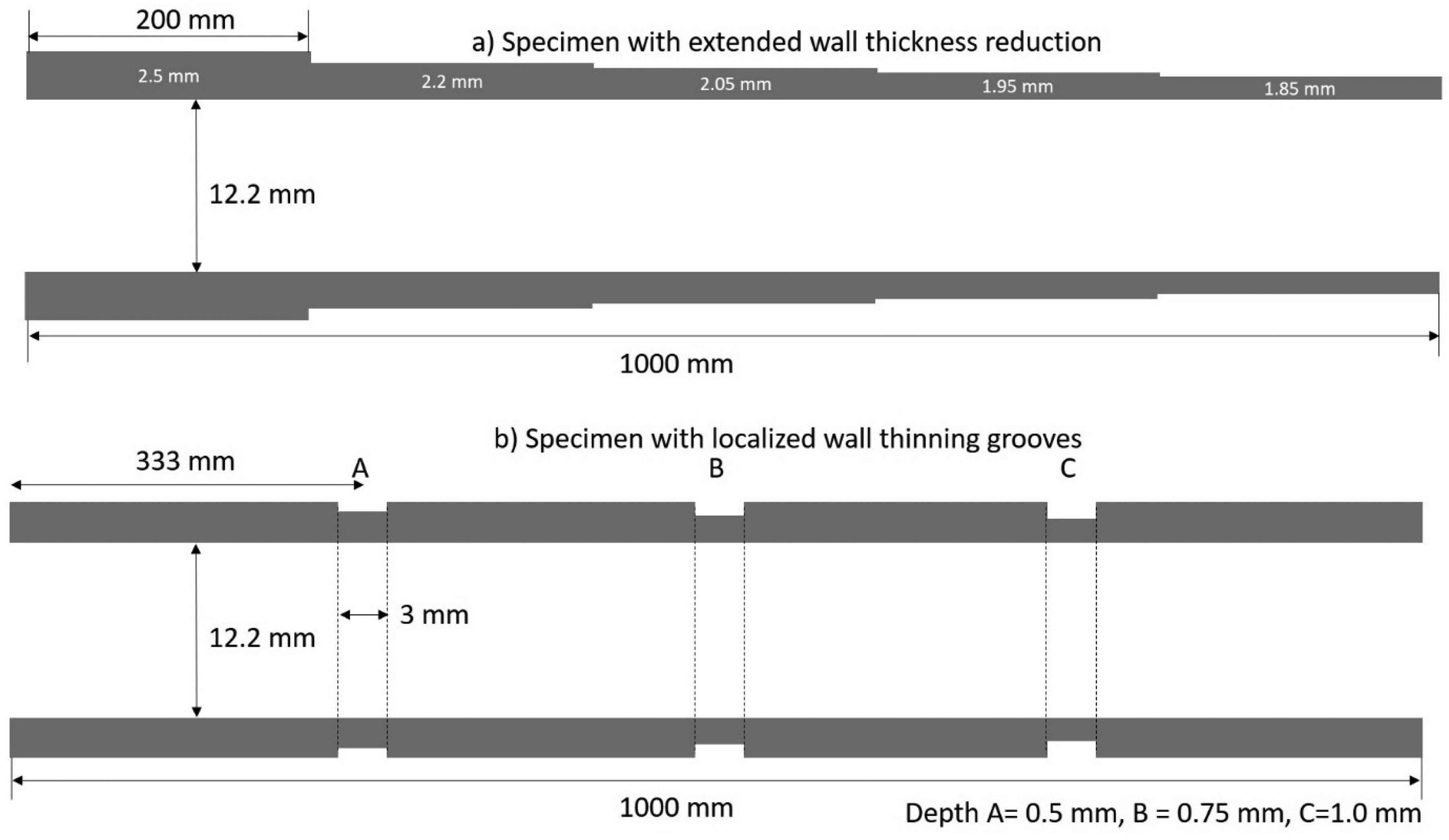
Schematic sketch of extended and localized wall thickness reduction in mod. 9Cr-1Mo steam generator tubes.

Results and discussion

Effect of excitation current on the nonlinear model

As indicated in Section 3 the excitation current was fixed at 100 mA following practical considerations. It is understood that the nonlinear effects for such an excitation current is negligibly small. To study this effect numerical experiments were performed, wherein the RFEC amplitude of a 20% wall loss groove was predicted for linear and nonlinear models for different excitation currents ranging from 50 mA – 500 mA (increase in the current will increase the magnetic field). Figure 4 shows the results of the study. As can be seen from the figure that there is a no deviation in the amplitude of the flaw between the linear and nonlinear models when the excitation currents are below 100 mA. Nonlinear effects are more pronounced beyond 100 mA currents. In this study, the excitation currents used in both the model-based analysis and the experimental setup are sufficiently low for the material to operate within the linear region of its B–H curve, where magnetic non-linearity is negligible. Consequently, extending the proposed methodology to strongly nonlinear regimes lie outside the scope of this study.

Figure 4.

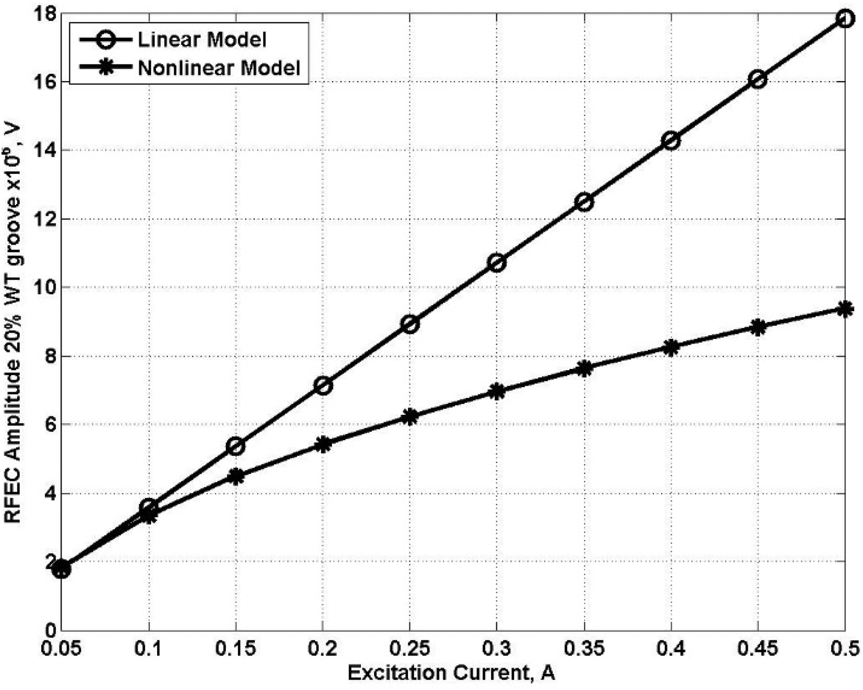
Variation of the model predicted amplitude of a 20% wall thinning groove in a steel tube for linear and nonlinear models.

Finite element model results

Figure 5(a) shows the model predicted inductive reactance changes of the probe as a function of excitation frequency for different thicknesses of the tube viz. 2.5 mm, 2.25 mm, 2.0 mm, 1.75 mm and 1.5 mm. In this case, the wall thickness reductions were made from the OD side of the tube. Figure 5(b) shows the simulation results for thickness reduction from the ID side of the tube. As envisaged, there exists a unique frequency for each thickness of the tube at which the reactance is maximum (peaks). This is because at lower and higher excitation frequencies on either side of the peak frequency, the eddy current density in the material becomes higher and offer higher secondary fields causing a reduction of impedance. At the peak frequency the current density is optimal for the selected tube thickness. This peak frequency (fp) is evaluated and is plotted as a function of percentage wall loss of the tube. Figure 6(a) shows variations in the peak frequency with wall thickness for both OD and ID thickness reductions. It can be seen in Figure 6(a) that the peak frequency quadratically increases with increase in percentage wall thickness reduction of the tube. This observation is in accordance with the skin-effect (Eq. 2):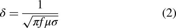

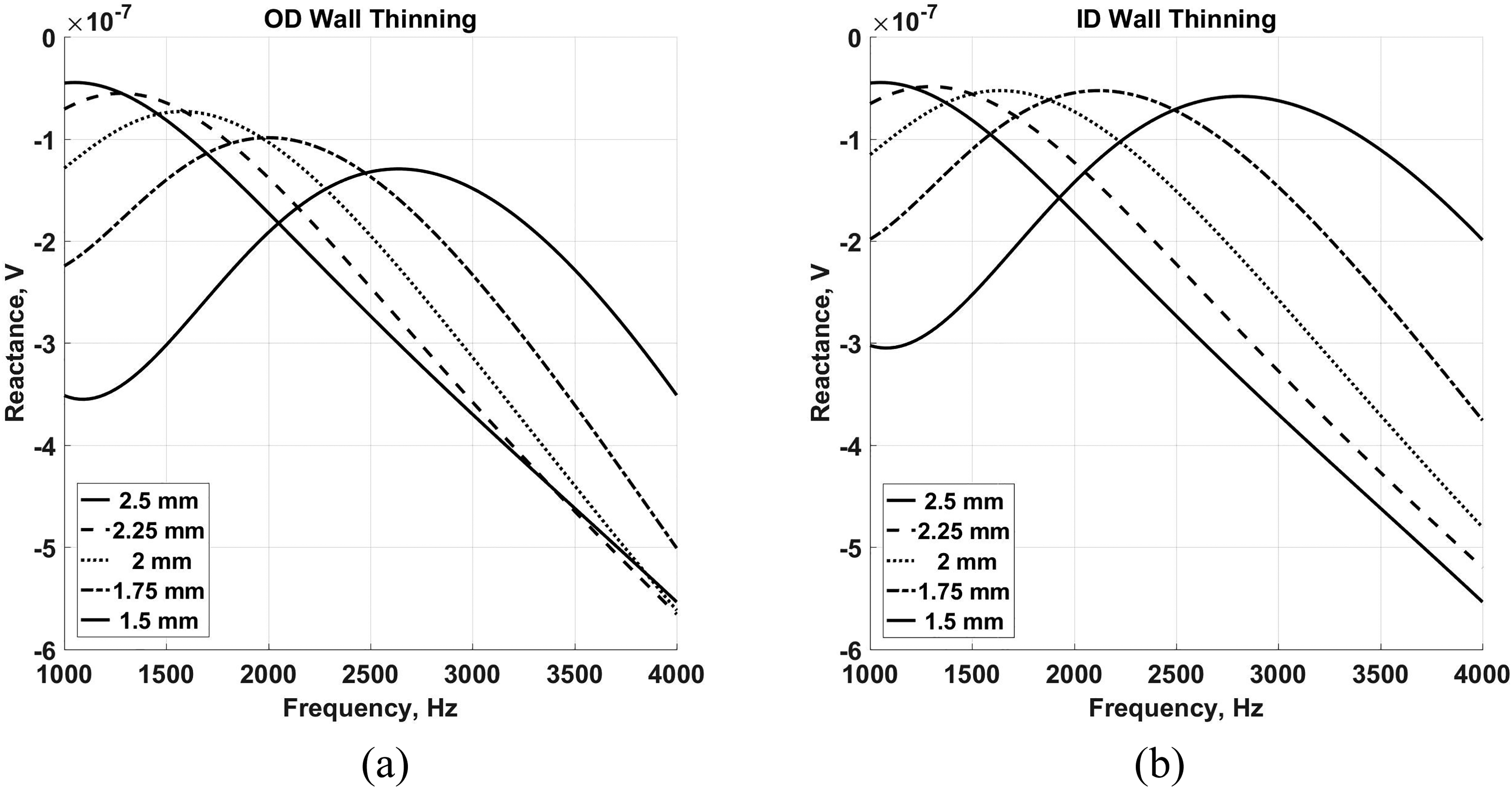
δ = \frac{1}{\sqrt{π f μ σ}}

(2)

where δ is standard depth of penetration of eddy currents, σ is electrical conductivity of the material and µ is the magnetic permeability of the material. As per the skin-effect theory, the depth of penetration of eddy currents in a material is inversely related to the square root of frequency (Eq. 2). Hence, to further confirm this behavior, a quadratic fit of peak frequency with wall loss was made. The R-squared value of the quadratic fit was found to be 99.93% and 99.91% for OD and ID wall thickness reductions respectively. Furthermore, a perfect linear relationship is observed between the inverse square root of peak frequency and wall loss as depicted in Figure 6(b). These observations confirm that the phenomenon is based on the skin-effect. An interesting observation is that the peak frequency changes are similar for both OD and ID wall thickness reductions especially for larger thickness regime. This is a characteristic of the RFEC technique that it is equally sensitive to ID and OD flaws. The minor deviation at lower thicknesses may be attributed to the changes in the RFEC behavior itself, when thickness changes are significant. These results clearly demonstrate that it is possible to accurately estimate the absolute thickness of the SG tubes using sweep frequency technique. An important point to be noted is that the results presented so far is applicable for extended wall thickness reduction and it is important to study this peak frequency behavior for localized wall thickness reduction.

Figure 5.

Variation of phase angle as a function of the frequency for different thickness for a) OD and b) ID extended wall thickness reduction.

Figure 6.

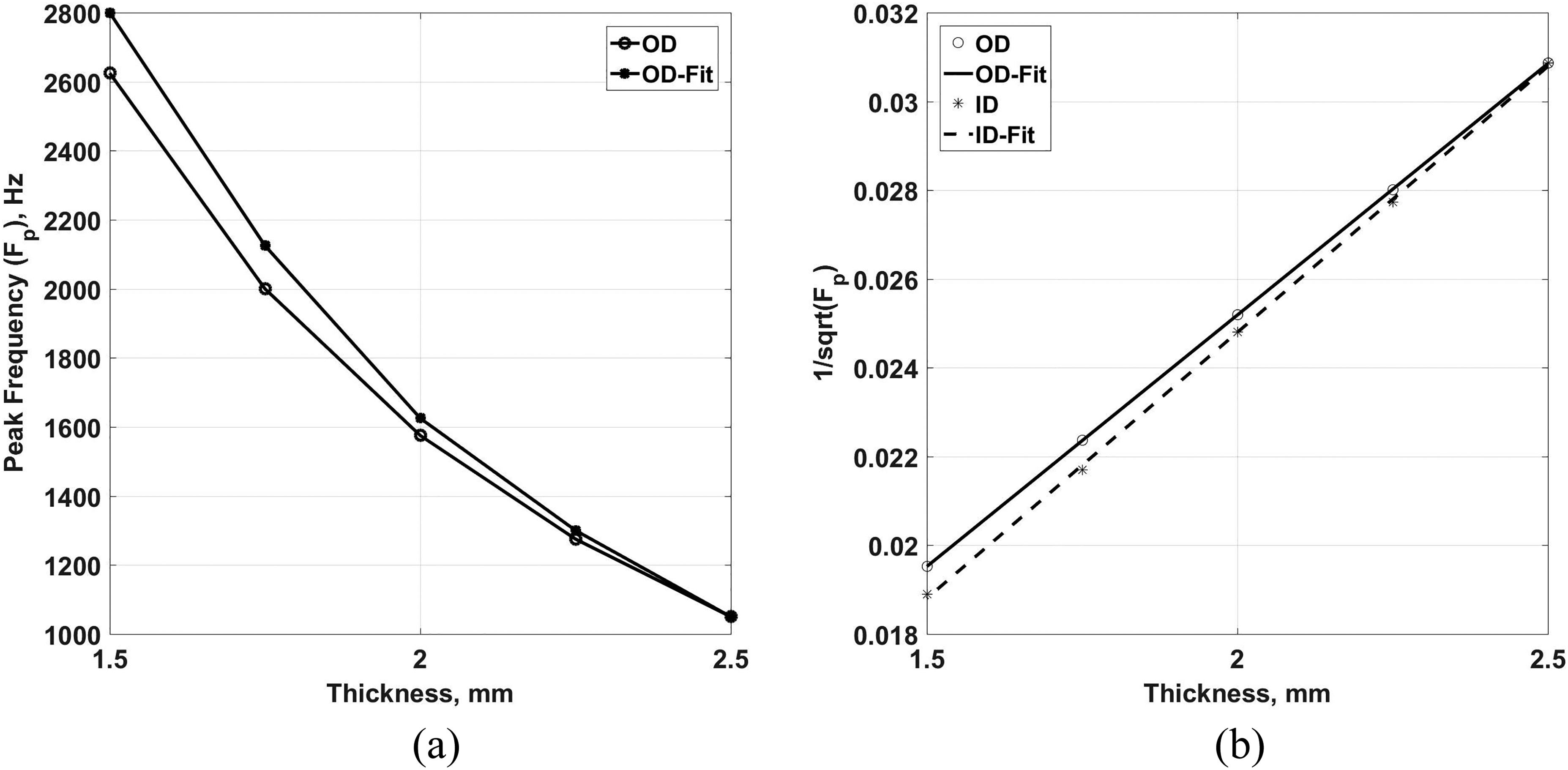
a) Peak frequency as a function of thickness with quadratic fit for OD and ID extended wall thickness reduction b) Linear variation of inverse square root of peak frequency with thickness for OD and ID extended wall thickness reduction.

In order to understand the peak frequency variation for localized wall thickness reduction, sweep frequency modeling was carried out for groove type localized OD and ID wall thickness reductions. The width of the grooves was kept at 2 mm, 5 mm, 10 mm and 30 mm for different remaining wall thickness values from 2.25 mm to 1.25 mm in steps of 0.25 mm. The frequency was swept from 1000 Hz to 2500 Hz when the receiver coil is placed exactly over the defect with centers of both the coil and defect matching. Figure 7(a) and (b) show the variation in reactance with frequency for OD and ID localized thickness reductions, respectively. Peaking behavior is seen for localized thinning also as observed from the figures and the results are like the case of the extended wall thickness reduction. Figure 8(a) shows the variations in inverse square root of peak frequency with thickness. In this case also, a perfect linear correlation is observed with percentage wall loss. However, the variations in peak frequency for OD and ID thickness reduction (Figure 8(b)) of the same width grooves are found to be significantly lower as compared to the extended wall thickness reduction. Careful observation of Figure 8 also reveals that this difference keeps on reducing as the width of the groove approach higher values.

Figure 7.

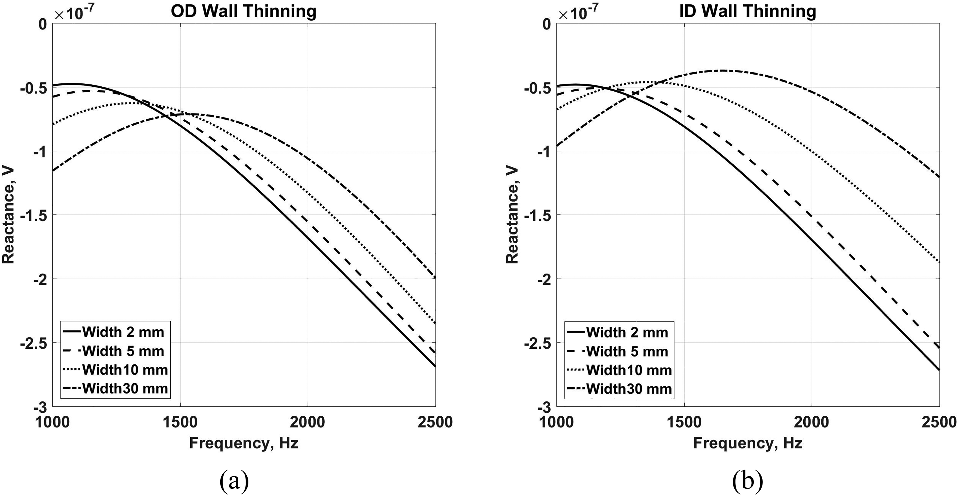
Variation of phase angle as a function of the frequency for different thickness for a) OD and b) ID localized wall thickness reduction.

Figure 8.

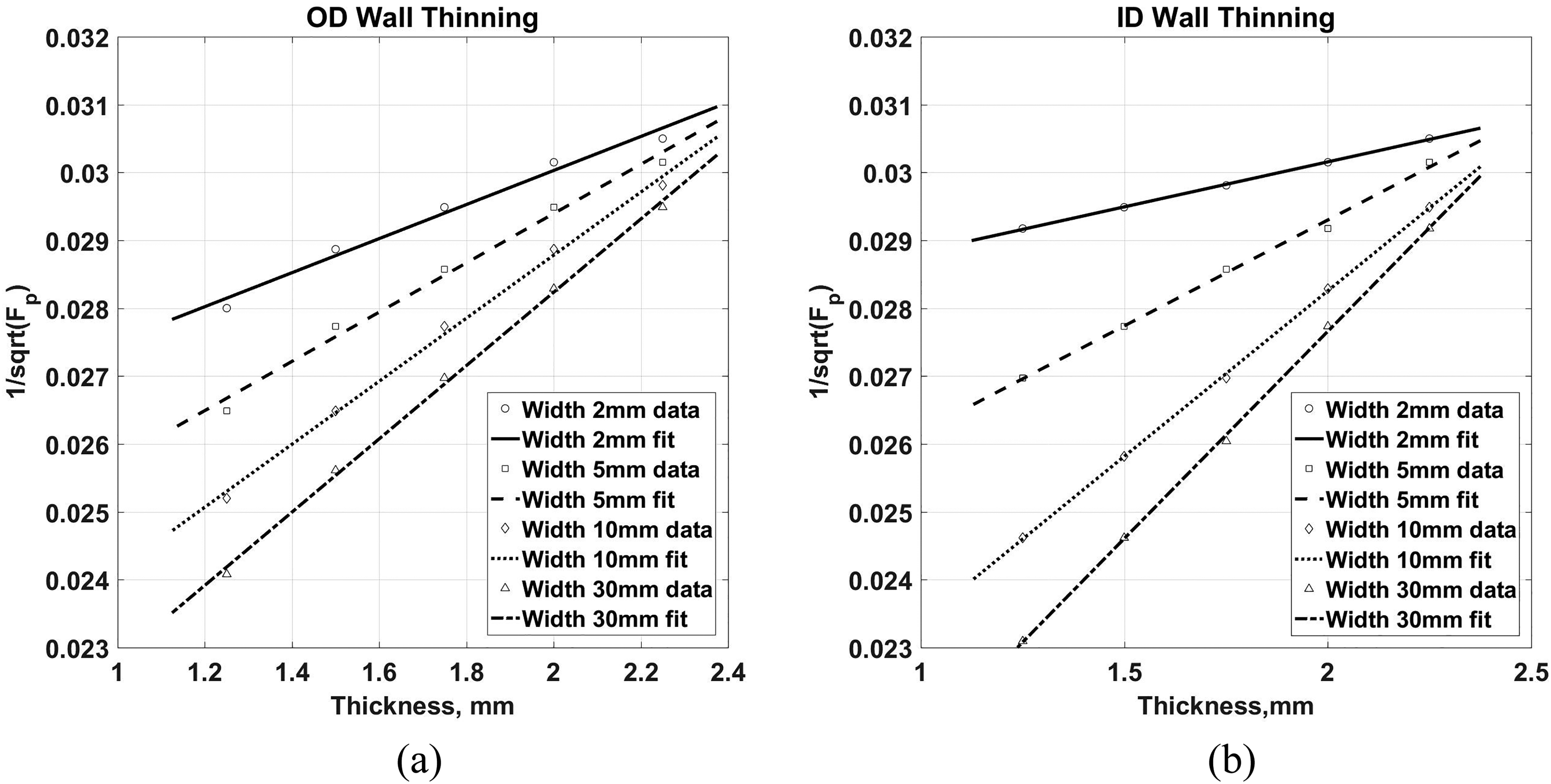
Linear variation of inverse square root of peak frequency with thickness for a) OD and b) ID localized wall thickness reduction.

Estimating the depth and width of the grooves

It is worth noting from Figure 6 that for each groove width the depth variation is associated with a unique straight line with slope (m) and intercept (c) values. Observation of the figure further reveals that the slopes of the straight lines decrease with in an increase in the width of the grooves and hence is a function of the groove width. This observation demonstrates that the width of the grooves influence thickness measurement by sweep frequency RFEC technique. However, the intercept values of all the straight lines are constant and is not a function of the groove width. These understandings aid in estimating the tube wall thickness (for known groove width) using the peak frequency parameter, with a parametric relation as given in equation (3):

D (W, f_{p}) = m (W) \sqrt{f_{p}} + c (W)

(3)

where D is the depth of grooves, W is the width of the groove, fp is the peak frequency, m and c are the slopes and intercepts values of the unique straight lines corresponding to each groove width. Equation (3) essentially aids in characterizing the depth of the grooves from the peak frequency parameter provided the width of the groove is known. Thus, it becomes important to find out the width of the grooves at the first instance for accurately sizing the depth or the remaining wall thickness. This can be achieved by making a sweep frequency line scan of the groove.

Figure 9 shows the model predicted peak frequency changes in a line scan made over a 50% wall loss groove of 2.5 mm width. The line scan begins at one end of the groove, with the front portion of the receiver coil aligned with the groove and continues to the other end until the trailing end of the exciter coil is aligned with the groove (as depicted in figure). The probe length used in this case is 47.5 mm (7.5 mm (Exciter length) + 35 mm (Spacing between exciter) + 5 mm (receiver length)), the scan length is 50 mm. We observe nearly identical peak frequency of 1070 Hz at the start and end of the line scan. The groove width can be estimated by subtracting the scan length and the probe length, which gives the width as 2.5 mm. Once the groove width is estimated this way, it becomes easy to estimate the depth of groove as given earlier using the straight-line calibration graph made for this width grooves. This study can also be extended to three dimensional flaws without any loss of generality wherein the depth of a rectangular flaw can be estimated knowing the length and width. However, further studies are necessary to simultaneously estimate the length and width using deconvolution or machine learning methods.

Figure 9.

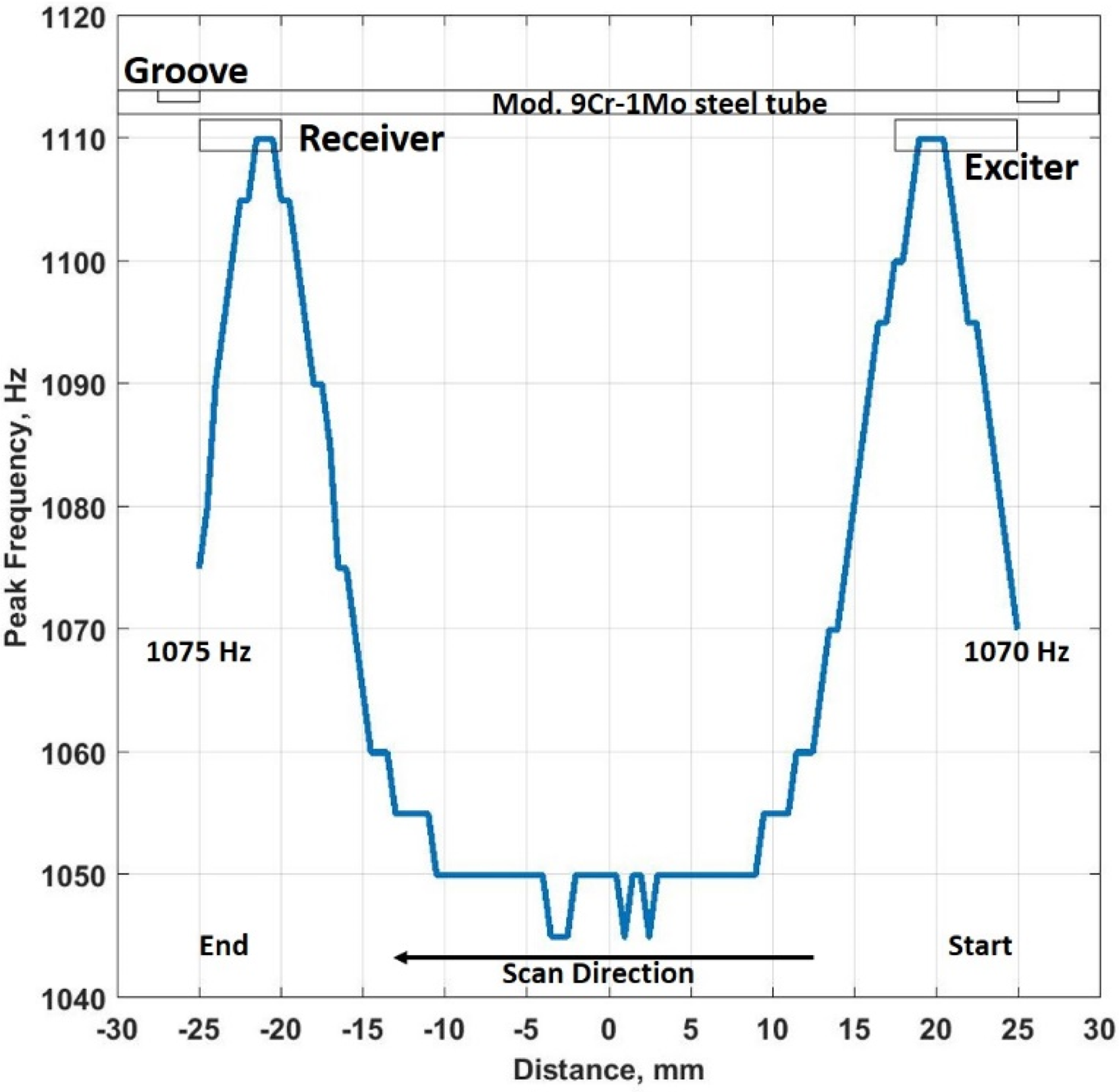
Peak frequency signal of a groove with axial distance.

Experimental results

Figure 10 (a) and (b) show the experimental measurements carried out on the extended wall thickness reduction. A unique peak frequency is observed for every thickness of the tube. The observed peak frequencies are 820 Hz, 1040 Hz, 1170 Hz, 1310 Hz and 1500 Hz for 2.5 mm, (0% wall loss), 2.2 mm (12% WL), 2.05 mm (18% WL), 1.95 mm (22% WL) and 1.85 mm (26% WL) thickness of the SG tube, respectively. As in the case of finite element modeling, a linear relationship is also observed between the thickness and inverse square root of the peak frequency. Figure 11 (a) and (b) show the same for groove type localized wall thickness reduction. The observed peak frequencies are 750 Hz, 775 Hz and 850 Hz respectively for the remaining wall thickness of the grooves of 2 mm (20%WL), 1.75 mm (25%WL) and 1.5 mm (40%WL). A linear relationship between thickness and inverse square root of frequency is also observed. In order to compare the experimental and model predictions the linear graph between the experimentally measured and model predicted peak frequencies are plotted with the tube thickness as shown in Figure 12. As can be seen there is a uniform offset between the model and the experimental results with the comparable slope values (within statistical fluctuations). This offset between the experimental and model results may be attributed to minor variations in the conductivity and permeability of the tube with respect to the measured ones used in the model. The experimental results are qualitatively in good agreement with the model predictions and demonstrate the feasibility of absolute and accurate thickness estimation of SG tubes by sweep frequency RFEC technique.

Figure 10.

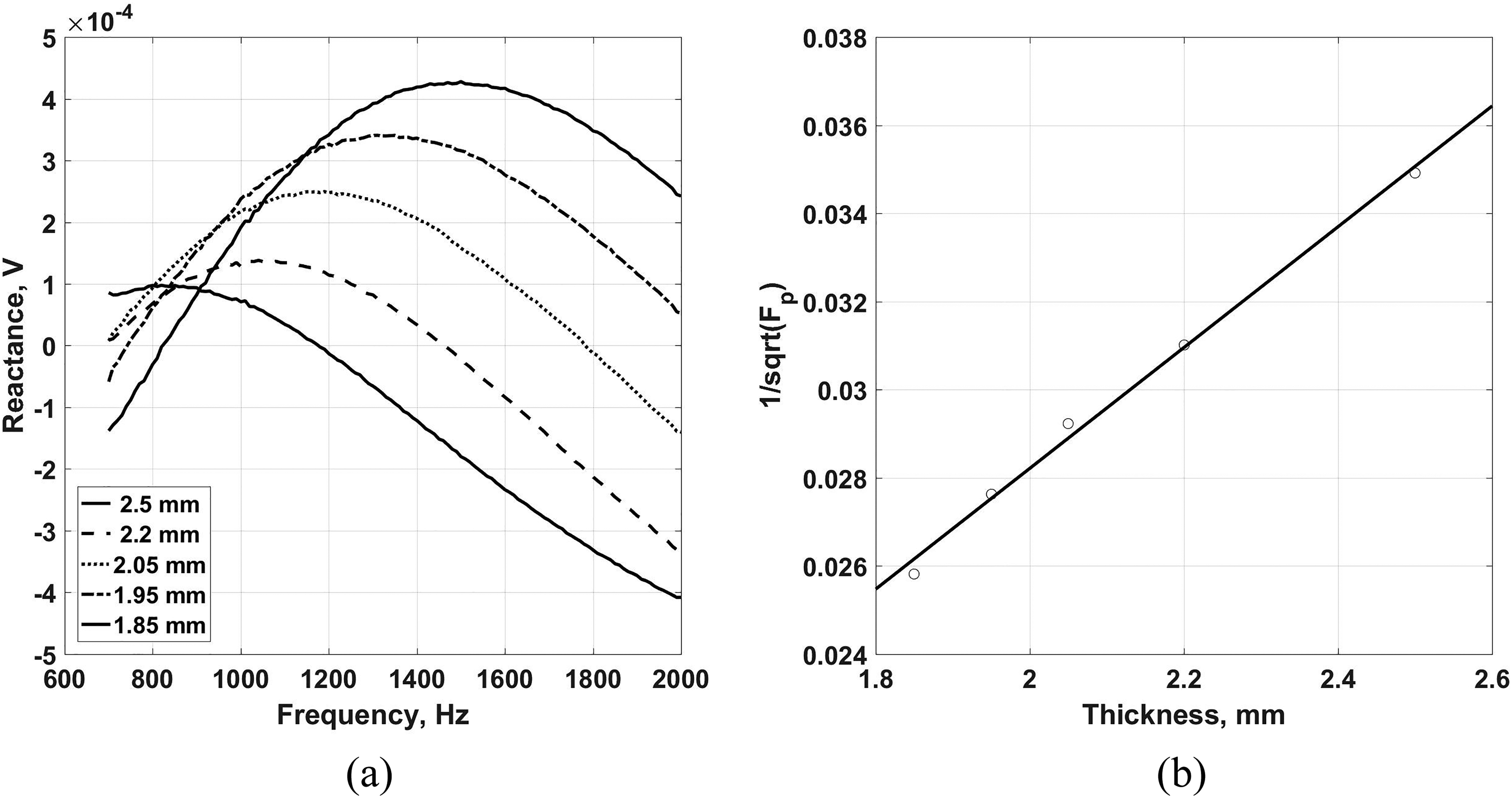
Sweep frequency RFEC measurements on tube specimen having extended wall thickness reduction.

Figure 11.

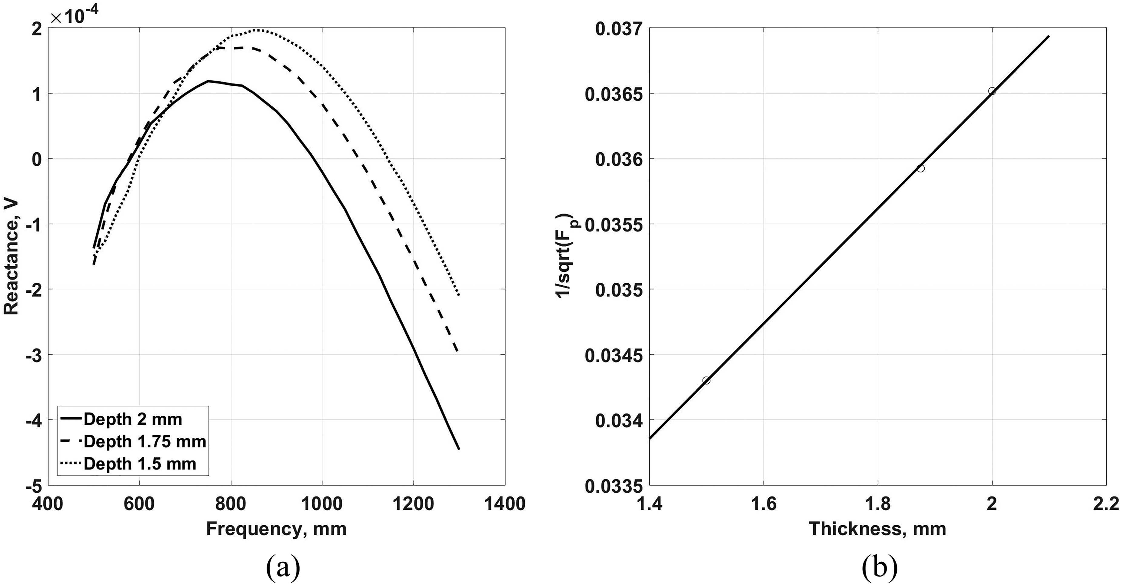
Sweep frequency RFEC measurements on tube specimen having localized uniform wall loss grooves.

Figure 12.

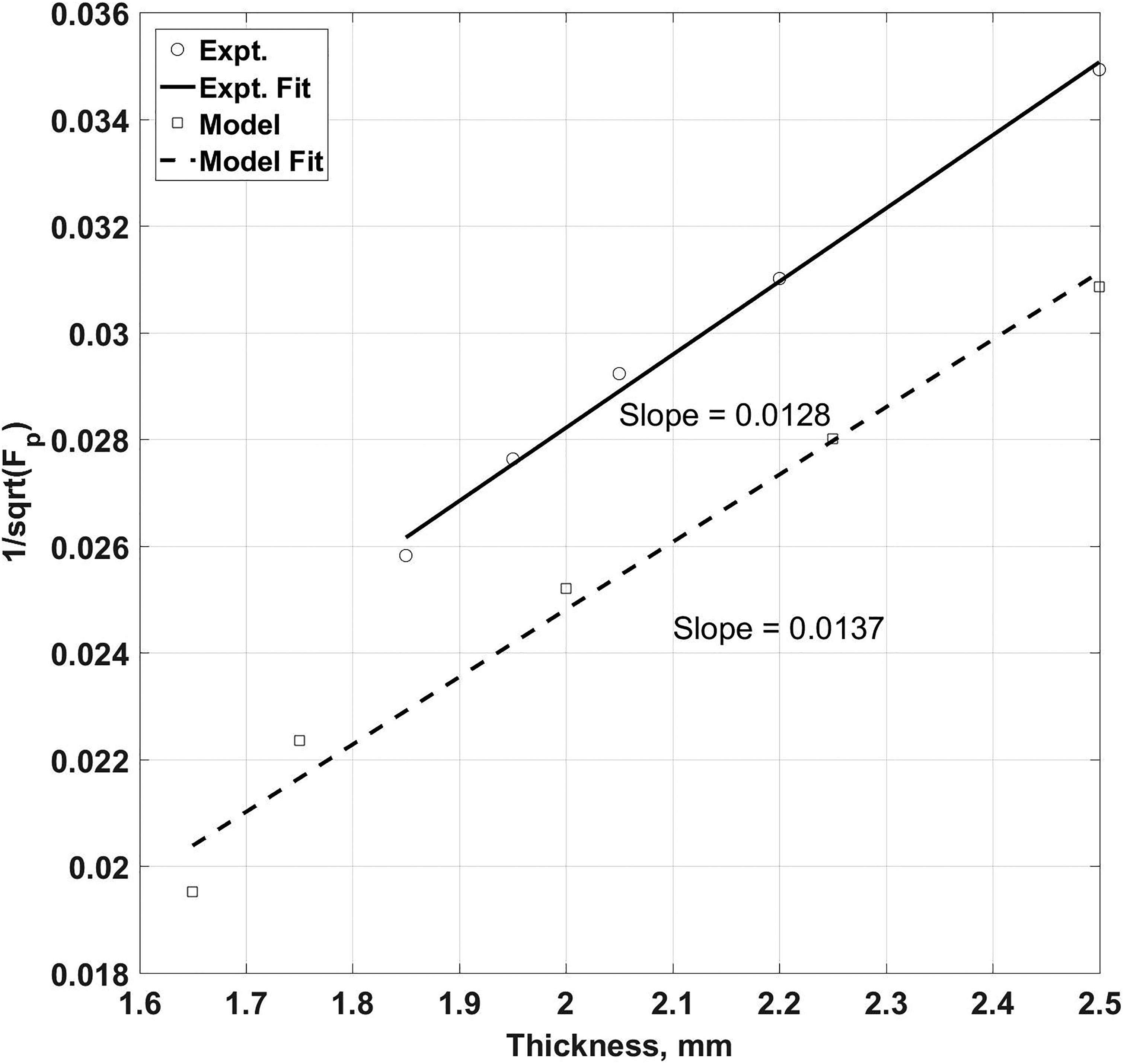
Comparison of model and experimental results.

Conclusions

Finite element model based and experimental studies were carried out to estimate thickness of ferromagnetic steam generator tubes using sweep frequency RFEC technique. Based on the axial extent, the thickness variations were categorized into extended and localized. Model based studies reveal that there exists a unique peak frequency for each thickness for extended thickness reductions and a linear correlation was observed between thickness and the inverse square root of the peak frequency following the skin-effect theory. Although similar observations could be made for the localized thickness reductions, the width or the length of the localized (flawed) region was found to influence the peak frequency parameter. This studied proposed a parametric linear relationship for estimation of absolute wall thickness with peak frequency, wherein the slope is a function of the groove width. Experimental studies have also confirmed this behavior and were in good agreement with the model predictions. Through this systematic approach, the study demonstrates how sweep-frequency measurements can significantly enhance flaw-sizing accuracy using a deterministic framework – an otherwise heavily ill-posed problem when relying solely on single-frequency measurements. The reported SF-RFEC results are first of its kind and shows promise for accurate and in-situ estimation of the remaining wall thickness of the tubes which is essential for condition monitoring of operating components such as the steam generator. This study focused on the sweep frequency behavior at lower excitation currents which are practically used, and the nonlinear magnetic effects are insignificant under the conditions considered.

Footnotes

ORCID iDs

S Thirunavukkarasu

Anish Kumar

Funding

The authors received no financial support for the research, authorship, and/or publication of this article.

Declaration of conflicting interests

The authors declared no potential conflicts of interest with respect to the research, authorship, and/or publication of this article.

References

Schmidt

. History of remote-field eddy current inspection technique. Mater Eval 1989; 47: 14–22.

Schmidt

. The casing inspection tool – an instrument for the in-situ detection of external corrosion in oil wells. Corrosion 1989; 17: 14–22.

Palanisamy

. Remote field eddy current testing – a review. Rev Progress Quantitat Nondestruct Evaluat 1988; 7: 157–164.

Thirunavukkarasu

Purna Chandra Rao

Joseph

, et al. Parametric sizing of tube wall thickness from multi-frequency remote field eddy current signals. Stud Appl Electromagn Mech June 2016; 41: 86–93.

Yin

Peyton

. Thickness measurement of non-magnetic plates using multi-frequency eddy current sensors. NDT&E Int 2007; 40: 43–48.

O'Kelly

. Hysteresis and eddy current losses in steel plates with nonlinear magnetization characteristics. Proc IEE November 1972; 119: 1675–1676.

Jack

Mecrow

. Methods for magnetically nonlinear problems involving significant hysteresis and eddy currents. IEEE Trans Magn March 1990; 26: 424–429.

Atherton

Czura

Lowther

. Open-boundary finite element calculations for remote field eddy current systems. IEEE Trans Magn September 1990; 26: 2863–2864.

Thirunavukkarasu

. Remote field eddy current based approaches for high sensitive detection of defects in ferromagnetic steam generator tubes. PhD dissertation, Homi Bhabha National Institute, Mumbai, India, http://www.hbni.ac.in/phdthesis/engg/ENGG02200704006.pdf (December, 2013).

10.

Thirunavukkarasu

Arjun

Purna Chandra Rao

, et al. Development of a high-sensitive dual frequency remote field eddy current instrument for inspection of ferromagnetic steam generator tubes. IETE Tech Rev 2019; 36: 203–208.