Functional linear mixed models for irregularly or sparsely sampled data

Abstract

We propose an estimation approach to analyse correlated functional data, which are observed on unequal grids or even sparsely. The model we use is a functional linear mixed model, a functional analogue of the linear mixed model. Estimation is based on dimension reduction via functional principal component analysis and on mixed model methodology. Our procedure allows the decomposition of the variability in the data as well as the estimation of mean effects of interest, and borrows strength across curves. Confidence bands for mean effects can be constructed conditionally on estimated principal components. We provide R-code implementing our approach in an online appendix. The method is motivated by and applied to data from speech production research.

Keywords

functional additive mixed models Dependent functional data functional principal component analysis penalized splines speech production

1 Introduction

Advancements in technology allow today's scientists to collect an increasing amount of data consisting of functional observations rather than single data points. Most methods in functional data analysis (fda) (see, e.g., Ramsay and Silverman 2005) assume that observations are (a) independent and/or (b) observed at a typically large number of the same (equidistant) observation points across curves.

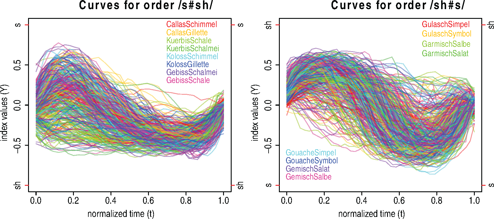
Linguistic research is only one of the numerous fields in which the data often do not meet these strong requirements. Our motivating data come from a speech production study (Pouplier et al. 2014) on assimilation, the phenomenon that the articulation of two consonants becomes more alike when they appear subsequently in spoken language. The data consist of audio recordings of nine speakers repeating the same 16 target words, including the two consonants of interest, each five times. The recorded acoustic signals during the duration of the two consonants were summarized by the phoneticians in a functional index over time (shown in Figure 1) varying between $+ 1$ and $- 1$ . Positive (negative) index values indicate proximity of the acoustic signal to a reference signal for the first (second) consonant of the target word. Thus, without assimilation, curves show a clear transition from strongly positive to strongly negative values. Assimilation can result in an earlier onset of the second consonant and/or a weakening of the first consonant, that is, smaller positive index values. In the extreme, curves become quite flat and only negative index values remain, indicating that the first consonant is dominated completely, possibly even replaced by the second. Due to the repeated measurements for speakers and for target words, the data have a crossed design structure. All recordings were taken with the same sampling rate, but the speaking durations differed. The index curves were thus standardized to a [0,1] time interval as changes relative to the length of the time interval (i.e., the duration of the consonant combination) are of interest. This results in different numbers and locations of the observation points between the observed curves.

We propose a model and an estimation approach that extend existing methods by accounting for both (a) correlation between functional data and (b) irregular spacing of—possibly very few—observation points per curve. The model is a functional analogue of the linear mixed model (LMM), which is frequently used to analyse scalar correlated data.

We use functional principal component analysis (FPCA; see, e.g., Ramsay and Silverman 2005) to extract the dominant modes of different sources of variation in the data. The functional random effects are expanded in bases of eigenfunctions of their respective auto-covariances, which we estimate beforehand using a novel smooth method of moments approach represented as an additive, bivariate varying coefficient model. FPCA is a key tool in fda as it yields a parsimonious representation of the data. It is attractive as the eigenfunction bases are estimated from the data and have optimal approximation properties for a fixed number of basis functions. It also allows for an explicit decomposition of the variability in the data.

We propose two ways of predicting the eigenfunction weights. We either compute them directly as empirical best linear unbiased predictors (EBLUPs) of the resulting LMM or we alternatively embed our previously estimated eigenfunctions and ’ values in the general framework of functional additive mixed models (FAMMs) introduced by Scheipl et al. (2015). The first approach is straightforward and computationally much more efficient; it does not require additional estimation steps as a plug-in estimate is used, and is thus almost a by-product of the eigenfunction estimation. The latter has the advantage that all model components are estimated/predicted in one framework, allowing for approximate statistical inference conditional on the FPCA.

There is previous work on dependent functional data as well as on functional data that is irregularly or sparsely observed, but with few exceptions noted below, existing work has not addressed both issues simultaneously.

First, methods for dependent functional data differ in their generality and in their restrictions on the sampling grid. Brumback and Rice (1998) consider a smoothing spline-based method for nested or crossed curves, which are modelled as fixed effect curves. They allow for missing observations in equal grids but do not consider any covariate effects. A Bayesian wavelet-based functional mixed model approach is introduced by Morris et al. (2003) and extended by Morris and Carroll (2006), Morris et al.(2006) and subsequent work by this group. While this approach is quite general in the possible functional random effects structure, and fixed and random effects are estimated within one framework allowing for full Bayesian inference, it assumes regular and equal grids with at most a small proportion of missings and a reasonable number of completely observed curves. Di et al. (2009), Greven et al.(2010) and Shou et al. (2015) consider functional linear mixed models (FLMMs) with a functional random intercept (fRI), with a fRI and functional random slope, and with nested and crossed fRIs, respectively. While following a similar approach to estimation of these models, all three are restricted to data sampled on a fine grid, and fixed effects are estimated under an independence assumption, not allowing for the statistical inference we provide. Di et al.(2014) extend the random intercept model of Di et al. (2009) to sparse functional data; the correlation structure, however, remains less general than ours and the estimation approach cannot easily be generalized to more complex structures. Also motivated by an application from linguistics, Aston et al. (2010) perform an FPCA on all curves ignoring the correlation structure, and then use the functional principal component (FPC) weights as the response variables in an LMM with random effects for speakers and words. Only linear effects of scalar covariates are considered, FPC bases are restricted to be the same for all latent processes, and it is assumed that the data are sampled on a common grid. Brockhaus et al. (2015) propose a unified class for functional regression models including group-specific functional effects, which are represented as linear array models, and are estimated using boosting. The array structure requires common grids and boosting does not provide inference. Other approaches concentrate specifically on spatially correlated functional data on equal grids, for example, Staicu et al. (2010). Scheipl et al. (2015) develop a flexible class of functional response models, allowing for various functional random effects with flexible correlation structures. Both spline-based and FPC-based representations are considered, and densely as well as sparsely sampled data are allowed. In the case of the FPC-based representation, they assume that appropriate FPC estimates are available. Yet, the estimation of the auto-covariances is challenging for correlated functional data with complex correlation structures, especially when observed on unequal grids, and no estimation approach is currently available. We combine our newly proposed FPC estimation with this general framework to obtain estimates, and approximate point-wise confidence bands (CBs) for the mean and covariate effects. In addition to providing an interpretable variance decomposition, our FPC-based approach reduces computation time by orders of magnitude compared to the spline-based estimates from Scheipl et al. (2015) (compare Section 5), allowing the analysis of realistically sized data in practice. Estimation errors and CB coverage also compare favourably.

Second, a number of approaches allow for irregularly or sparsely sampled functional data but assume that curves are independent. (Guo 2002, Guo 2004) first introduces the term functional mixed effects models for his model. The model does not capture between-function correlation as only curve-level random effect functions are included, which are modelled using smoothing splines. The approach is not restricted to regularly sampled grid data. Chen and Wang (2011) propose a spline-based approach that is suitable for sparsely sampled data, but similar to Guo (2002); Guo (2004), they only consider curve-level random effects. James et al. (2000), Yao et al. (2005) and Peng and Paul (2009) among others propose FPCA approaches for sparsely observed functional data with uncorrelated curves. For functional data with independent curves, there is a direct relationship to the longitudinal data literature as well, too extensive to cover here.

For an extensive overview and further references for functional regression approaches, including functional response regression, see Morris (2015).

The remainder of the article is organized as follows. Section 2 introduces the general FLMM and presents an important special case which is used to analyse the motivating linguistic data on assimilation. Section 3 develops our estimation framework. Our method is evaluated in an application to the assimilation data and in simulations in Sections 4 and 5, respectively. Section 6 closes with a discussion and outlook. Theoretical results and supplementary material including estimation details as well as additional results for application and simulations are available in the online appendix, where we also provide R-code implementing our approach.

2 Functional linear mixed models

2.1 The general model

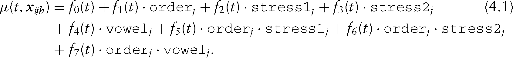
The general FLMM is given by

Y_{i} (t) = μ (t, x_{i}) + z_{i}^{⊤} U (t) + E_{i} (t) + ε_{i} (t), i = 1, \dots, n,

(2.1)

where

Y_{i} (t)

is the square-integrable functional response observed at arguments

t

T

, a closed interval in

, and

n

is the number of curves.

μ (t, x_{i})

is a fixed main effect surface dependent on a vector of known covariates

x_{i}

of length

p

. To account for the functional nature of the

Y_{i} (t)

, the random effects of an LMM are replaced by a vector-valued random process

U (t)

z_{i}

is a known covariate vector of length

q

E_{i} (t)

is a curve-specific deviation in the form of a smooth residual curve. We assume that there is a white noise measurement error denoted by

ε_{i} (t)

with variance

σ^{2}

that captures random uncorrelated variation within each curve. Note that if needed, the error variance may also vary across

t

σ^{2} (t)

. We further assume that

U (t)

E_{i} (t)

and

ε_{i} (t)

i = 1, \dots, n

are zero-mean, square-integrable, mutually uncorrelated random processes, which assures model identification. Therefore, each of the

q

components of

U (t)

has an auto-covariance operator

K^{U_{j}} (t, t^{'})

j = 1, \dots, q

, and cross-covariance operators

K^{U_{j, k}} (t, t^{'})

j, k = 1, \dots, q

, some of which might be zero for uncorrelated functional random effects.

E_{i} (t)

has an auto-covariance operator

K^{E} (t, t^{'}) = Cov [E_{i} (t), E_{i} (t^{'})]

. In the following, mean, auto-covariances and thus also the eigenfunctions are assumed to be smooth in

t

. For any given

t

, model (2.1) with our assumptions corresponds to an LMM with general mean

μ (x_{i})

$μ (t, x_{i})$ is an additive function of $t$ and $x_{i}$ . For example, it can be constant in $t$ , $μ (t, x_{i}) = μ (x_{i})$ , or additive in $t$ and $x_{i}$ , $μ (t, x_{i}) = μ_{1} (t) + μ_{2} (x_{i})$ . Another special case is when all $x_{i 1}, \dots, x_{ip}$ in $x_{i}$ act as index-varying coefficients, $μ (t, x_{i}) = f_{0} (t) + f_{1} (t) x_{i 1} + \dots + f_{p} (t) x_{ip}$ , with unknown smooth functions $f_{0} (\cdot), \dots, f_{p} (\cdot)$ .

2.2 Special case: The FLMM for a crossed design

For our application in speech production research (Section 4), we use an FLMM with a crossed design structure to account for correlation between measurements of the same speaker and between measurements of the same target word.

Y_{ijh} (t) = μ (t, x_{ijh}) + B_{i} (t) + C_{j} (t) + E_{ijh} (t) + ε_{ijh} (t),

(2.2)

with

i = 1, \dots, I

(number of speakers),

j = 1, \dots, J

(number of target words) and

h = 1, \dots, H_{i j}

(number of repetitions). Here,

Y_{ijh} (t)

is the

h

th index curve for speaker

i

and target word

j

observed at time

t

B_{i} (t)

and

C_{j} (t)

are fRIs for the speakers and target words, respectively. Curve-specific deviations are accommodated by the smooth residual term

E_{ijh} (t)

, which also captures interactions between speakers and target words. Based on substantive considerations and the limited sample size, we decided not to include an interaction effect separately.

ε_{ijh} (t)

is additional white noise measurement error with variance

σ^{2}

. We denote the auto-covariance operators by

K^{B} (t, t^{'}) = Cov [B_{i} (t), B_{i} (t^{'})]

K^{C} (t, t^{'}) = Cov [C_{j} (t), C_{j} (t^{'})]

and

K^{E} (t, t^{'}) = Cov [E_{ijh} (t), E_{ijh} (t^{'})]

i = 1 \dots, I

j = 1, \dots, J

h = 1, \dots, H_{i j}

2.3 Irregularly and sparsely sampled functional data

Let us now assume that for our general model (2.1), we have observed $n$ curves on observation points ${t_{i 1}, \dots, t_{{iD}_{i}}} \in T, i = 1, \dots, n$ . The number and the location of the observation points are allowed to differ from curve to curve. In the extreme, only one point may be observed for a curve. Moreover, the observation points of a curve do not have to be equally spaced. We denote realizations of the functional response $Y_{i} (t)$ at point $t_{i j}$ by $y_{{it}_{i j}}, j = 1, \dots, D_{i}$ . Accordingly, we denote realizations of the response in model (2.2) by $y_{ijht}$ with $t \in {t_{ijh 1}, \dots, t_{{ijhD}_{ijh}}}$ .

3 Estimation

We base our estimation on FPCA, which provides the dimension reduction so important for functional data and allows an explicit decomposition of the variability. Compared to other basis approaches, for example, using splines, FPCA has the advantage that the eigenbases are optimal in the sense of giving the best approximation for a given number of basis functions, and thus typically small numbers of basis functions give good approximations. To pool information across observations, which is particularly important in the case of irregularly or sparsely sampled functional data, we use smoothing of the auto-covariances of $U (t)$ and $E_{i} (t)$ , cf. Yao et al. (2005) for non-correlated sparse functional data. Previous approaches for smoothing the auto-covariances are restricted to less complex correlation structures or data sampled on an equal, fine grid. We apply eigen decompositions of the auto-covariances based on Mercer's theorem (Mercer 1909). The eigenfunctions, also known as FPCs, describe the main modes of variation of processes $U (t)$ and $E_{i} (t)$ , and the eigenvalues quantify the amount of variability explained by the corresponding FPCs. The eigenfunction weights, or FPC weights, give insight into the individual structure of each grouping level and can be used in further analyses, for example, classification. The four main steps of our estimation procedure are outlined as follows:

Step 1
We estimate the mean $μ (t, x_{i})$ using penalized splines based on a working independence assumption.
Step 2
We use a smooth method of moments estimator based on the centred curves to estimate the auto-covariances of the functional random effects.
Step 3
We conduct an eigen decomposition of each estimated auto-covariance matrix evaluated on a pre-specified, fine grid. Using the Karhunen-Loève (KL) expansion (Loève 1945; Karhunen 1947), we represent the functional random effects in truncated bases of eigenfunctions.
Step 4
We propose two ways of predicting the random basis weights.

Step 1, Step 3 and the first option for Step 4 are analogous to the estimation proposed in Di et al. (2009), Greven et al. (2010) and Shou et al. (2015) for functional data sampled on an equal, fine grid and in Di et al. (2014) for a simpler model. Step 2 is new and leads to a new combination with the FAMM approach of Scheipl et al. (2015) in the second option for Step 4. For simplicity, we focus in the remainder of this section, where we describe the four steps in detail, on model (2.2).
3.1 Step 1: Estimation of the mean function

We estimate the mean $μ (t, x_{ijh})$ based on the working independence assumption

Y_{ijh} (t) = μ (t, x_{ijh}) + ε_{ijh} (t),

(3.1)

with independent and identically distributed (i.i.d.) Gaussian random variables

ε_{ijh} (t)

. Model (3.1) is an additive model with additive mean

μ (t, x_{ijh}) = f_{0} (t) + \sum_{k = 1}^{p} f_{k} (t) x_{ijhk}

. We represent the unknown, smooth functions

f_{k} (\cdot)

using B-splines, and control the trade-off between goodness of fit and smoothness by adding a difference penalty (so-called P-splines; Eilers and Marx 1996). Using the penalized splines approximation of model (3.1) allows us to represent the model as a scalar LMM, which has the advantage that the smoothing parameter can be estimated as a variance component ratio using restricted maximum likelihood (REML; Patterson and Thompson, 1971; cf. Ruppert et al., 2003, sec. 4.9). We centre the data using the estimated mean

\hat{μ} (t, x_{ijh})

and obtain

{\tilde{y}}_{ijht} : = y_{ijht} - \hat{μ} (t, x_{ijh})

. For more general mean models than varying coefficient models, see Wood et al. (2015).

3.2 Step 2: Estimation of the auto-covariances

We estimate the auto-covariances using a smooth method of moments estimator. Whereas for data sampled on an equal, fine grid, estimation can be done point-wise, this is not possible for irregularly or sparsely sampled data, which makes the estimation of the auto-covariances more challenging and requires a new approach. We exploit the fact that for centred data, the expectation of the cross products corresponds to the auto-covariance, which can be decomposed as follows:

\begin{array}{l} E [{\tilde{Y}}_{i j h} (t) {\tilde{Y}}_{i^{'} j^{'} h^{'}} (t^{'})] = C o v [{\tilde{Y}}_{i j h} (t), {\tilde{Y}}_{i^{'} j^{'} h^{'}} (t^{'})] \\ = K^{B} (t, t^{'}) δ_{i i^{'}} + K^{C} (t, t^{'}) δ_{j j^{'}} + [K^{E} (t, t^{'}) + σ^{2} δ_{t t^{'}}] δ_{i i^{'}} δ_{j j^{'}} δ_{h h^{'}}, \end{array}

(3.2)

with δ_xx equal to one if

x = x^{'}

and zero otherwise. We propose to see (3.2) as an additive, bivariate varying coefficient model, in which the auto-covariances are the unknown smooth bivariate functions to be estimated, while

δ_{{ii}^{'}}, δ_{{jj}^{'}}, δ_{{ii}^{'}} δ_{{jj}^{'}} δ_{{hh}^{'}}

and

δ_{{ii}^{'}} δ_{{jj}^{'}} δ_{{hh}^{'}} δ_{{tt}^{'}}

represent the covariates. Under a working assumption of independence and homoscedastic variance of the cross products, we can use each empirical product

{\tilde{y}}_{ijht} {\tilde{y}}_{i^{'} j^{'} h^{'} t^{'}}

for which at least

i = i^{'}

j = j^{'}

to obtain smooth estimates of

K^{B} (t, t^{'})

K^{C} (t, t^{'})

and

K^{E} (t, t^{'})

, and an estimate of the error variance

σ^{2}

. The total number of products

{\tilde{y}}_{ijht} {\tilde{y}}_{i^{'} j^{'} h^{'} t^{'}}

used for the estimation of the auto-covariances is of order

O (D^{2} (1 / I + 1 / J))

, with

D

being the total number of observation points.

We use bivariate tensor product P-splines (see, e.g., Wood 2006 sec. 4.1.8) for the estimation of the auto-covariances, where low rank marginal bases for each $t, t^{'}$ are combined in order to obtain smooth functions of the two covariates. Let $\otimes$ denote the Kronecker product. Then, given the appropriate ordering of the parameter vector, the part of the design matrix corresponding to $K^{X} (t, t^{'})$ , $X \in {B, C, E}$ , is given by the respective indicator matrix multiplied entry-wise by $(M_{t}^{X} \otimes 1_{F^{X}}^{⊤}) \cdot (1_{F^{X}}^{⊤} \otimes M_{t^{'}}^{X})$ , where $M_{t}^{X}$ and $M_{t^{'}}^{X}$ denote the corresponding marginal spline design matrices of rank $F^{X}$ for covariate $t$ and $t^{'}$ , and $1_{F^{X}} = {(1, \dots, 1)}^{⊤}$ of length $F^{X}$ . A smoothness penalty is introduced in order to avoid over-fitting. To account for the natural symmetry of the auto-covariances, we choose an isotropic penalty with a penalty matrix of the form $S_{{tt}^{'}} = S_{t} \otimes S_{t^{'}}$ , where $S_{t}$ and $S_{t^{'}}$ represent the respective marginal penalty matrices for $t$ and $t^{'}$ . For reasons of model complexity and computational feasibility, we use marginal B-spline bases combined with marginal difference penalties. In principle, other bases or smoothing techniques are possible, which also applies to the estimation of the mean in Step 1. We take advantage of the mixed model representation of model (3.2) for the estimation of the tensor product basis coefficients and the smoothing parameter using REML. During the estimation, strength is borrowed across all curves. This can be extremely advantageous for sparse functional data when some curves only have very few measurements, and smoothing of curves would be infeasible. In practice, negative estimated values of $σ^{2}$ are set to zero for the final estimate. Symmetry of the auto-covariances is ensured through the model apart from numerical inaccuracies.

For the practical implementation of Step 1 and Step 2, we build on existing software and use R-function (R Development Core Team 2014) bam, implemented in the R-package mgcv (Wood 2011) which is especially designed for large data sets. Avoiding the construction of the complete design matrix leads to a low memory footprint, and the possibility of parallelization gives a considerable speed-up in computation time. For further details, see Wood et al. (2015).

3.3 Step 3: Eigen decompositions of estimated auto-covariances

Based on Mercer's Theorem, the eigen decompositions of the auto-covariances are

K^{X} (t, t^{'}) = \sum_{k = 1}^{\infty} ν_{k}^{X} ϕ_{k}^{X} (t) ϕ_{k}^{X} (t^{'}), X \in {B, C, E},

where,

ν_{1}^{X} \geq ν_{2}^{X} \geq \dots \geq 0

are the respective eigenvalues,

k \in

. The corresponding eigenfunctions

{ϕ_{k}^{X}, k \in}

X \in {B, C, E}

, form an orthonormal basis in the Hilbert space

L^{2} [T]

with respect to the

L^{2}

-scalar product

⟨ f, g ⟩ = \int f (t) g (t) d t

. In practice, the smooth auto-covariances are evaluated on an equally spaced, dense grid

{t_{1}, \dots, t_{D}}

of pre-specified length

D

. The resulting matrices are in the following denoted as

{\hat{K}}^{X} = {[{\hat{K}}^{X} (t_{d}, t_{d^{'}})]}_{d, d^{'} = 1, \dots, D}

X \in {B, C, E}

. We conduct an eigen decomposition of each estimated auto-covariance matrix yielding estimated eigenvectors and eigenvalues. Rescaling is necessary to ensure that the approximated eigenfunctions are orthonormal with respect to the

L^{2}

-scalar product. Negative estimated eigenvalues are trimmed to zero to guarantee positive semi-definiteness.

Truncation of the FPCs: While in theory, there is an infinite number of eigenfunctions, dimension reduction achieved by the selection of the number of FPCs for each random process is necessary in practice. This truncation has a theoretical justification and can be seen as a form of penalization (see, e.g., Di et al. 2009; Peng and Paul 2009). Among the multiple proposals in the literature (see for an overview Greven et al. 2010), we base our choice on the proportion of variance explained. This allows us to quantify the contribution of the random processes to the variation in the observed data. It is based on the variance decomposition of the response

\int_{T} Var [Y_{ijh} (t)] d t = \sum_{k = 1}^{\infty} ν_{k}^{B} + \sum_{k = 1}^{\infty} ν_{k}^{C} + \sum_{k = 1}^{\infty} ν_{k}^{E} + σ^{2} | T | .

The sums

\sum_{k = 1}^{\infty} ν_{k}^{X}

X \in {B, C, E}

, quantify the relative importance of each of the three random processes. We choose principal components of decreasing importance until a pre-specified level of explained variation is reached.

Approximation of the functional random processes: Based on the truncation, we use KL expansions to obtain parsimonious basis representations for the random processes

B_{i} (t) \sum_{k = 1}^{N^{B}} ξ_{ik}^{B} ϕ_{k}^{B} (t), C_{j} (t) \sum_{k = 1}^{N^{C}} ξ_{jk}^{C} ϕ_{k}^{C} (t), E_{ijh} (t) \sum_{k = 1}^{N^{E}} ξ_{ijhk}^{E} ϕ_{k}^{E} (t) .

Note that in the case of irregularly or sparsely sampled data, the observation points

t

also depend on

i

j

and

h

, which we omit throughout this article for better readability. For the same reason, we do not emphasize that the truncation lags and eigenfunctions are estimated. By construction, the basis weights

ξ_{ik}^{B}

ξ_{jk}^{C}

and

ξ_{ijhk}^{E}

are uncorrelated random variables with zero mean and variance

ν_{k}^{X}

k \in

X \in {B, C, E}

For prediction of the FPC weights, we first linearly interpolate the chosen eigenfunctions such that they are available on the original observation points. Due to the smoothness of all model components, this leads to a small error which could be further decreased, if desirable, by further increasing the number of grid points $D$ .

See Online Appendix B for further details, including the rescaling of the FPCs, and Online Appendix A for the derivation of the variance decomposition.

3.4 Step 4: Prediction of the basis weights

The basis weights for a centred random process $X_{i} (t)$ are often represented as the scalar product of $X_{i} (t)$ and the respective FPC. Estimation is more complicated for dependent functional data contaminated with additional measurement error as the weights belonging to the different basis expansions cannot be separated, and ignoring the measurement error leads to biased predictions. Moreover, numerical integration would not work (well) for irregularly or sparsely sampled data.

These considerations motivate our two proposals for the prediction of the basis weights. The first is straightforward and computationally very efficient. It is almost a by-product of the FPC estimation, taking only a few seconds for our large phonetics data. It generalizes the conditional expectations introduced by Yao et al. (2005). The second involves higher computational costs but has the advantage that the mean is re-estimated in the same framework, allowing for approximate statistical inference, for example, for the construction of point-wise CBs conditional on the FPCA. Depending on the sample size of the data and the main question of interest, one or the other may be preferred. Further details for both, such as concrete matrix forms, can be found in Online Appendix A.

Prediction of the basis weights as EBLUPs: Using the truncated KL expansions of the random processes, we can approximate model (2.2) by

Y_{ijh} (t) μ (t, x_{ijh}) + \sum_{k = 1}^{N^{B}} ξ_{ik}^{B} ϕ_{k}^{B} (t) + \sum_{k = 1}^{N^{C}} ξ_{jk}^{C} ϕ_{k}^{C} (t) + \sum_{k = 1}^{N^{E}} ξ_{ijhk}^{E} ϕ_{k}^{E} (t) + ε_{ijh} (t)

(3.3)

for the discrete observation points

t \in {t_{ijh 1}, \dots, t_{{ijhD}_{ijh}}}

. The resulting model (3.3) is a scalar LMM in which the random effects correspond to the basis weights (Di et al. 2009). The basis weights are directly predicted as EBLUPs without fitting model (3.3), plugging in the previously estimated components, as derived in the following. Note that without normality assumption, the predictors remain best linear predictors.

Let $\tilde{Y}$ denote the stacked centred response vector of length $D$ . Let $L^{X} \in {I, J, n}$ and $N^{X} \in {N^{B}, N^{C}, N^{E}}$ denote the levels of the grouping variable and the truncation lag for process $X$ , $X \in {B, C, E}$ , respectively. We define $ξ = {(ξ^{B^{⊤}}, ξ^{C^{⊤}}, ξ^{E^{⊤}})}^{⊤}$ , with $ξ^{X} = {({ξ_{1}^{X}}^{⊤}, \dots {, ξ_{L^{X}}^{X}}^{⊤})}^{⊤}$ being the stacked vector of the basis weights of length $L^{X} N^{X}$ . Thus, $ξ$ is a vector of length $N : = {IN}^{B} + {JN}^{C} + {nN}^{E}$ . $\hat{Φ}$ is the joint $D \times N$ design matrix of the form $\hat{Φ} = [{\hat{Φ}}^{B} | {\hat{Φ}}^{C} | {\hat{Φ}}^{E}]$ , where ${\hat{Φ}}^{B}$ , ${\hat{Φ}}^{C}$ and ${\hat{Φ}}^{E}$ are the respective design matrices containing the rescaled FPC estimates evaluated on the original observation points. $\hat{G}$ denotes the estimated covariance matrix of $ξ$ . It is a diagonal matrix with elements corresponding to the estimated eigenvalues of the random processes.

The EBLUP for the basis weights in model (2.2) in the usual form (see Online Appendix A) requires the inversion of the estimated covariance matrix of $\tilde{Y}$ , which is of dimension $D \times D$ . This can be computationally demanding for large numbers of observation points. Furthermore, when ${\hat{σ}}^{2} 0$ , the covariance becomes singular. Transformations with the Woodbury formula yield the more favourable form

\hat{ξ} = {({\hat{σ}}^{2} \hat{G} + {\hat{Φ}}^{⊤} \hat{Φ})}^{- 1} {\hat{Φ}}^{⊤} \tilde{Y},

(3.4)

for which the inversion is simplified to that of an

N \times N

matrix which has full rank when either

{\hat{σ}}^{2}

is positive or when

{\hat{Φ}}^{⊤} \hat{Φ}

has full rank. In practice, when neither of these requirements is met, the Moore-Penrose generalized inverse is used. Note that when

{\hat{σ}}^{2} = 0

, the EBLUP simplifies to the least-squares estimator.

This computationally efficient way of predicting $ξ$ can be used when the focus is not on inference for covariate effects or when the data are large and the computational resources are limited. One drawback is, however, that the mean is estimated using a working independence assumption. This may not be statistically efficient and does not directly provide valid statistical inference. This motivates our second proposal.

Prediction of the basis weights using FAMMs: The second option uses the fact that model (3.3) together with the distribution of the basis weights implied by the KL expansion falls into the general framework of a FAMM (Scheipl et al. 2015) using suitable marginal bases and penalties. We combine our FPC estimation with the FAMM idea, and write model (3.3) using estimated eigenfunctions and -values as

Y = \sum_{k = 0}^{p} (Ψ_{c}^{k} \otimes 1_{F^{k}}^{⊤}) \cdot Ψ_{t}^{k} θ^{k} + \sum_{X \in {B, C, E}} (Ψ_{g}^{X} \otimes 1_{N^{X}}^{⊤}) \cdot (1_{L^{X}}^{⊤} \otimes Ψ_{t}^{X}) ξ^{X} + ε,

(3.5)

with

ε \sim N (0, σ^{2} I_{D})

Y

is the stacked uncentred response vector of length

D

, and the mean is re-estimated with

Ψ_{c}^{k}

denoting an inflated vector of length

D

of covariate values.

Ψ_{t}^{k}

of dimension

D \times F^{k}

comprises the evaluations of

F^{k}

spline basis functions on the

D

time points

t_{ijh}

θ^{k}

is a coefficient vector of length

F^{k}

. For the functional random effects,

Ψ_{g}^{X}

denotes an inflated

D \times L^{X}

matrix of grouping indicators. The

D \times N^{X}

matrix

Ψ_{t}^{X}

comprises the evaluations of the

N^{X}

respective estimated eigenfunctions on the original observation points. Adding penalties of the form

{ξ^{X}}^{⊤} (I_{L^{X}} \otimes P_{t}^{X}) ξ^{X}

with

P_{t}^{X} = diag {({\hat{ν}}_{1}^{X}, \dots, {\hat{ν}}_{N^{X}}^{X})}^{- 1}

corresponds to the distributional assumption

ξ_{l}^{X} \sim N (0, diag ({\hat{ν}}_{1}^{X}, \dots, {\hat{ν}}_{N^{X}}^{X}))

l = 1, \dots L^{X}

X \in {B, C, E}

, implied by the KL expansions under Gaussianity. This set-up using linear combinations of the above tensor product bases with an appropriate penalty falls naturally into the framework of a FAMM, and was in fact discussed in Scheipl et al. (2015) without, however, providing an approach to the estimation of the eigenfunctions and -values needed in

Ψ_{t}^{X}

and

P_{t}^{X}

. Model (3.5) is a scalar additive LMM, which allows to take advantage of established methods for estimation and for statistical inference (for more details, see Scheipl et al. 2015). Re-estimation of the mean in one framework with the basis weights, particularly allows us to construct point-wise CBs for the mean and for covariate effects. Note that the inference is conditional on the estimated FPCA, that is, it accounts neither for the uncertainty in the estimated eigenfunctions and -values nor for the truncation, which may lead to an underestimation of the variability. (Compare, however, the good coverage in our simulations in Section 5.2). In practice, we use function pffr that Scheipl et al. 2015 provide in the R-package refundDevel (Crainiceanu et al. 2014). A constraint on the functional random effects assures that they are centred. In addition to the parsimonious basis of eigenfunctions, this approach has the advantage of not necessitating the estimation of any smoothing parameters for the random processes, as the variances of the random weights have already been estimated and the smoothing parameter can be set to one. These two features lead to a drastic decrease in computational cost compared to spline-based prediction of the random processes, as is shown in our simulations in Section 5.

The estimation quality can be further improved, if desirable, by applying the four estimation steps iteratively. Several possibilities are described in Online Appendix B, where further details on the estimation and implementation can also be found.

4 Application to the speech production research data

4.1 Background and scientific questions

In linguistics, the term assimilation refers to the common phenomenon whereby a consonant becomes phonetically more like an adjacent, usually following consonant. Assimilation commonly occurs in English phrases such as ‘Paris show’ in which the word-final /s/-sound is, in fluent speech, pronounced very similar to the following, word-initial /sh/-sound (Pouplier et al. 2011). Assimilation patterns are conditioned by a complex interaction of perceptual, articulatory and language-specific factors, and are therefore a central research topic in the speech sciences. In order to investigate assimilation in German, Pouplier et al. (2014) obtained audio recordings of $I = 9$ speakers reading the same $J = 16$ target words, each five times. Due to the recording errors, for some combinations, only four repetitions are included in the data, that is, $H_{i j} \in {4, 5}$ . The authors concentrated on variation in assimilation patterns for the consonants /s/, /sh/ as a function of their order (/s#sh/ versus /sh#s/, where # denotes a word boundary), syllable stress and vowel context. Target words consisted of bisyllabic noun-noun compounds. In half of the target words, consonant /s/ is followed by word-initial /sh/, such as in the word ‘Callas-Schimmel’. The other half contains the sequence /sh#s/, for example, ‘Gulasch-Symbol’. In the following, we will refer to the syllables containing the consonants of interest as final and initial target syllables (and correspondingly to final and initial target consonants). The time interval in which the consonants of interest appear in the utterance was cut out manually from the audio recording for each repetition and the resulting time-varying acoustic signal was summarized in a functional index over time, varying between $+ 1$ and $- 1$ . Reference patterns for both the consonants were used to construct the index such that it ranges for both orders from $+ 1$ for sounds close to the reference for the first consonant of the sequence to $- 1$ for sounds close to the reference for the second consonant of the sequence (for more details, see Pouplier et al. (2011) and Online Appendix C for data pre-processing). The resulting index curves are displayed in Figure 1.

Figure 1

Index curves of the consonant assimilation data over time. Left [right]: Curves of order /s#sh/ [/sh#s/]. Positive values approaching $+ 1$ indicate a reference /s/ [/sh/] acoustic pattern, while negative values approaching $- 1$ indicate a reference /sh/ [/s/] acoustic pattern.

A special focus lies on the asymmetry arising from the order of the consonants. We investigate under which conditions (order, syllable stress, vowel context) the two consonants assimilate, and whether assimilation is symmetric with respect to the orders /s#sh/ and /sh#s/. A common approach is to extract curve values at pre-defined points on the time axis (e.g., 25%, 50%, 75%) which are subsequently used in multivariate methods (e.g., Pouplier et al. 2011 ). Such analyses fail to capture the continuous dynamic change characteristic of speech signals. Applying our fda-based method allows us to take into consideration the temporal dynamics and to account for the complex correlation structure in the data which arises from the repeated measurements of speakers and of target words. Moreover, we can quantify the effect of covariates and interactions and obtain a variance decomposition.

All utterances were recorded with the same sampling rate (32 768 Hz) and then standardized to a [0,1] interval as the speaking rate, and hence the target consonant duration, differs across experiments. After standardization, measurements are unequally spaced for different curves. In some data settings, registration can be used to account for variation in time. For this application, however, registration cannot replace the standardization of the time interval as different transition speeds between the two consonants are part of the research question of interest and thus a change relative to the length of the time interval is of interest. Registration would remove the main source of information on the assimilation process and flat curves, arising from (near) complete assimilation, would render registration problematic.

4.2 A model for the consonant assimilation data

In order to account for the repeated measurements of speakers and target words, we fit an FLMM with crossed fRIs, model (2.2), to the consonant assimilation data. The number of measurements per curve $D_{ijh}$ ranges from 22 to 57 with a median of 34. During estimation, we truncate the numbers of FPCs using a pre-specified proportion of explained variance of $0.95$ . The equidistant grid on which the auto-covariances are evaluated is of length $D = 100$ . We use cubic B-splines with third order difference penalties for the estimation of the mean effects and as marginal basis functions for the estimation of the auto-covariances. We predict the FPC weights using both options. As CBs for the covariate and interaction effects are of interest here, the focus lies on the second approach using the FAMM framework.

Covariate effects: We consider four dummy-coded covariates: consonant order (order), stress of the final (stress1) and of the initial (stress2) target syllable, which can be strong or weak and vowel context (vowel), which refers to the vowels immediately adjacent to the target consonants and is either of the form ia or ai, for example, Callas-Schimmel. Moreover, we include the interactions of the consonant order with each of the other three covariates. All covariates enter the mean as varying coefficients,

\begin{array}{l} μ (t, x_{i j h}) = f_{0} (t) + f_{1} (t) \cdot o r d e r_{j} + f_{2} (t) \cdot stress 1_{j} + f_{3} (t) \cdot s t r e s s 2_{j} \\ + f_{4} (t) \cdot {vowel}_{j} + f s (t) \cdot {order}_{j} \cdot stress 1_{j} + f_{6} (t) \cdot {order}_{j} \cdot stress 2_{j} \\ + f_{7} (t) \cdot {order}_{j} \cdot {vowel}_{j} . \end{array}

(4.1)

Thus, in total, eight covariates characterize the 16 target words.

4.3 Application results

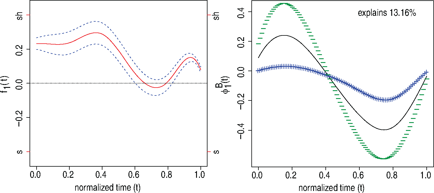
Our estimation yields two and three FPCs for the fRI for speakers and for the smooth error, respectively. No FPC is chosen for the fRI for target words. It is likely that the eight covariate and interaction effects describe the target words sufficiently, as confirmed by obtaining one FPC for the fRI for target words in the model without covariate effects. Most variability (67.29%) is explained by the three chosen FPCs for the curve-specific deviation which also captures interactions between speakers and target words. The two chosen FPCs for speakers explain 20.45% of the estimated variability.

The left panel of Figure 2 shows the effect of covariate order ( $f_{1}$ ), which has the largest effect on the index trajectories. Covariate order is dummy-coded with reference category /s#sh/. Thus, the mean curves of target words with order /sh#s/ are pulled towards the ideal reference /sh/ during the first consonant and differ slightly from the ideal /s/ during the second consonant compared to order /s#sh/. We conclude that there is an asymmetry of consonant assimilation with respect to the consonant order and that /s/ is more affected by the assimilation than /sh/. These results are consistent with the results for English obtained by Pouplier et al. (2011).

Figure 2

Left: Effect of covariate order (red solid line) with point-wise confidence bands (dashed lines). Right: Mean function (solid line) and the effect of adding ( $+$ ) and subtracting ( $-$ ) a suitable multiple ( $2 \sqrt{{\hat{ν}}_{1}^{B}}$ ) of the first FPC for speakers.

Moreover, we find that assimilation is stronger for target words with unstressed final syllables ( $f_{2}$ ), especially for order /s#sh/ ( $f_{5}$ ). Changing the stress of the initial syllable only has an effect for order /sh#s/ ( $f_{6}$ ). This means that in both final and initial position, stress effects are evident during /s/ but not during /sh/. For order /s#sh/, the vowel context mainly affects the transition between the two consonants ( $f_{4}$ ). The first consonant is closer to the ideal reference value in the ai compared to the ia condition, yet the second consonant is pulled away from its reference value. Changing the vowel context does not affect order /sh#s/ beyond edge-effects ( $f_{7}$ ). This shows that word-final /s/, but not /sh/ is affected by the vowel condition.

In the right panel of Figure 2, we show the effect of adding ( $+$ ) and subtracting ( $-$ ) a suitable multiple of the first FPC for speakers to the overall mean (solid line) obtained by setting all covariates to 0.5. The interpretation is straightforward: speakers with a negative weight for the first FPC distinguish better between the two consonants. The estimates for the basis weights can be used for further analysis. Further application results including plots for all mean effects can be found in Online Appendix C.

5 Simulations

5.1 Simulation designs

We conduct extensive simulation studies to investigate the performance of our method. The data generating processes can be divided into two main groups: (a) data that mimics the irregularly sampled consonant assimilation data and (b) sparsely sampled data with a higher number of observations per grouping level but fewer observations per curve. For all settings, we generate 200 data sets.

Application-based simulation scenarios: We consider two application-based scenarios, one with an fRI for speakers and covariate mean effects (fRI scenario) and another with crossed fRIs for speakers and for target words, respectively, but no covariate mean effects (crossed-fRIs scenario). We generate the data based on the estimates of model (2.2) for our consonant assimilation data with $μ (t, x_{ijh})$ corresponding to Section (4.1) and to a simple smooth intercept $μ (t)$ , respectively. The data analysis yields two FPCs for the fRI for the speakers and three FPCs for the smooth error term. For the crossed-fRIs scenario, we additionally obtain one FPC for the fRI for the target words. The FPC weights and the measurement errors are independently drawn from normal distributions with zero mean and with the respective estimated variances. To assess the effect of model misspecification, we conduct additional simulations of the crossed-fRI scenario, using FPC weights drawn from a mixture of two normals, with equal probability from either $N (\sqrt{ν_{k} / 2}, ν_{k} / 2)$ or $N (- \sqrt{ν_{k} / 2}, ν_{k} / 2)$ as in Yao et al. (2005). We obtain very similar results to the corresponding results for normal weights, and the curves can be reconstructed equally well. More details on the data generation can be found in Sections 4.3, 5.2 and in Online Appendices C and D.

Sparse simulation scenario: In order to investigate the estimation performance in the sparse case, we additionally generate data with crossed fRIs as in model (2.2) consisting of observations that are sparsely sampled on [0,1]. The number of observation points per curve is drawn from the discrete uniform distribution $U {3, 10}$ . For $B_{i} (t)$ and $C_{j} (t)$ , we choose $I = J = 40$ replications each with each combination observed $H_{i j} = 3$ times. We use two FPCs each to generate the underlying process. Eigenvalues are generated as $ν_{k}^{X} = 2 / k, k = 1, 2$ , $X \in {B, C, E}$ . We choose normalized Legendre polynomials adapted to the interval $[0, 1]$ as FPCs for $B_{i} (t)$ and $C_{j} (t)$ . For the smooth error $E_{ijh} (t)$ , we choose a basis of sine and cosine functions. See Online Appendix D for details. The FPC weights and the measurement errors are independently drawn from the normal distributions $N (0, ν_{k})$ and $N (0, σ^{2})$ , respectively. No covariates are included in the mean function $μ (t) = sin (t) + t$ . We set the error variance to $σ^{2} = 0.05$ .

For all scenarios, we centre the FPC weights such that the weights of each grouping variable also empirically have zero mean. Moreover, we decorrelate the basis weights belonging to one grouping variable and assure that the empirical variance corresponds to the respective eigenvalue. This is done to obtain data that meet the requirements of our model. It allows us to separate the effect of unfavourably drawn weights and of the estimation performance. This adjustment gains importance for small sample sizes $I$ , $J$ and $n$ and also when the true eigenvalues are high. Note that in practice, we do not have centred and decorrelated FPC weights, and thus estimates for small sample sizes will reflect the distribution in the sample rather than that in the population. To assess the impact of this procedure, we also compare our results to those of simulations using the original (non-centred and non-decorrelated) FPC weights, which can be found in Online Appendix D.

We fix the number of FPCs in order to separate the effect of the truncation from the estimation quality. We use five marginal basis functions each for the estimation of the auto-covariances and eight basis functions for the estimation of the mean. We predict the FPC weights as EBLUPs for all scenarios, and additionally compare with the computationally more expensive FAMM prediction (FPC-FAMM) for the fRI scenario with covariates.

We compare our FPC-based approach to a spline basis representation of the functional random effects (using eight basis functions) within the FAMM framework of Scheipl et al. (2015) (spline-FAMM). To the best of our knowledge, the work of Scheipl et al. (2015) is the only competitor to our approach as all other methods are either restricted to equal, fine grids or do not allow for a crossed structure. Due to the high computational costs of Scheipl et al. (2015), we restrict our comparison to the fRI scenario, in which we can compare estimation quality and CBs coverage for covariate effects.

5.2 Simulation results

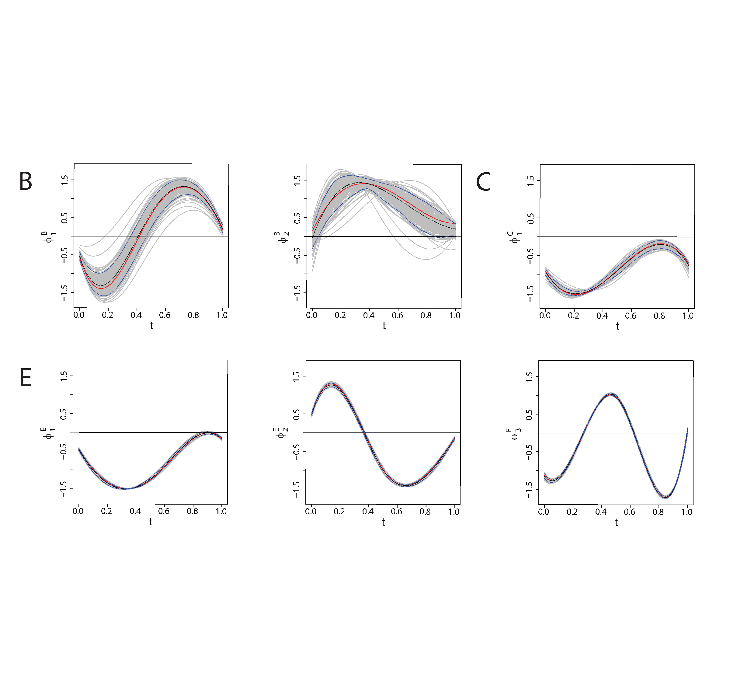
We focus our discussion on the FPC-based results for the application-based scenario with crossed fRIs and compare with the other settings and estimation approaches. We use root relative mean squared errors (rrMSE) as measures of goodness of fit which are of the general form $\sqrt{{(true - estimated)}^{2} / {true}^{2}}$ . For the simulations of the fRI scenario with covariate effects, we additionally evaluate the average point-wise and the simultaneous coverage of the point-wise CBs. The complete results for all simulations as well as rrMSE definitions for scalars, vectors and functions are given in Online Appendix D.

Simulation results for the crossed-fRIs scenario: Figure 3 shows the true and estimated FPCs of the two fRIs as well as of the smooth error term. As expected, the better the FPCs are estimated, the more independent levels are there for the corresponding grouping variable which can enter the estimation of the auto-covariance. The FPCs of the smooth error term (707 levels) are estimated best, followed by the FPC of the fRI for target words (16 levels). 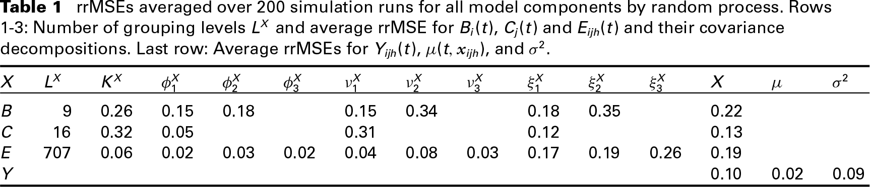Most variability in the estimates is found for the FPCs of the fRI for speakers due to the small number of speakers ( $I = 9$ ), but the main features of the curves are still recovered relatively well. We obtain similar results for the fRI scenario. The number and complexity of the FPCs also play an important role for the estimation quality, as can be seen from the results for the sparse scenario, where the first FPC of $B_{i} (t)$ (40 levels) is estimated better than the first FPC of $E_{ijh} (t)$ (4800 levels). The latter has a more complex form, difficult to capture with five basis functions.

Table 1 lists the rrMSEs averaged over 200 simulation runs for all model components. It shows that the mean function is reconstructed very well, which is also the case in the sparse scenario. The covariate effects for the fRI scenario are discussed below. The auto-covariances and their eigenvalues have similar low average rrMSEs for both application-based scenarios. For the sparse scenario, the eigenvalues are estimated even better with average rrMSEs between 0.02 and 0.05. For the auto-covariances for the sparse scenario, we obtain average rrMSEs of 0.06 for each of the crossed fRIs and an average of 0.14 for the smooth error which is due to the complex eigenfunctions mentioned above. The error variance has similar low average rrMSEs for the two application-based scenarios. For the sparse scenario, the average rrMSE is higher, which is due to the estimation inaccuracies in the auto-covariance of the smooth error.

Table 1

rrMSEs averaged over 200 simulation runs for all model components by random process. Rows 1-3: Number of grouping levels L^X and average rrMSE for $B_{i} (t)$ , $C_{j} (t)$ and $E_{ijh} (t)$ and their covariance decompositions. Last row: Average rrMSEs for $Y_{ijh} (t)$ , $μ (t, x_{ijh})$ , and $σ^{2}$ .

$X$	$L^{X}$	$K^{X}$	$ϕ_{1}^{X}$	$ϕ_{2}^{X}$	$ϕ_{3}^{X}$	$ν_{1}^{X}$	$ν_{2}^{X}$	$ν_{3}^{X}$	$ξ_{1}^{X}$	$ξ_{2}^{X}$	$ξ_{3}^{X}$	$X$	$μ$	$σ^{2}$
$B$	9	0.26	0.15	0.18		0.15	0.34		0.18	0.35		0.22
$C$	16	0.32	0.05			0.31			0.12			0.13
$E$	707	0.06	0.02	0.03	0.02	0.04	0.08	0.03	0.17	0.19	0.26	0.19
$Y$												0.10	0.02	0.09

The prediction quality of the basis weights clearly depends on the estimation quality of the FPCs and of the eigenvalues, as well as of the error variance, as evident from equation 3.4). Also important for the prediction of the basis weights is the number of curves with the given weight entering the prediction. Thus, the basis weights of $C_{j} (t)$ are better predicted than those of $E_{ijh} (t)$ . As expected, basis weights of FPCs that explain more variability are predicted better. Similar results can be found for the fRI and for the sparse scenario.

For all scenarios, we obtain good results for the functional random effects as well as for the functional response. The rrMSEs for the functional response are lowest, which is due to the fact that even if the FPC bases are not perfectly estimated, they can still serve as a good empirical basis. Thus, the data can be reconstructed very well.

We found considerably more outliers of the relative errors for the sparse scenario than for the other two scenarios, which is most probably due to an unfavourable distribution of the few observation points across the curves in a few data sets.

Figure 3

True and estimated FPCs of the crossed fRIs $B_{i} (t)$ and $C_{j} (t)$ (top row), as well as of the smooth error $E_{ijh} (t)$ (bottom row). Shown are the true functions (red solid line), the mean of the estimated functions over 200 simulation runs (black dashed line), the point-wise 5th and 95th percentiles of the estimated functions (blue dashed lines) and the estimated functions of all 200 simulation runs (grey).

Overall, we can conclude that all components are estimated well and especially for the functional response we obtain very small rrMSEs across all simulations.

Comparison of the different estimation results for the fRI scenario: We find that the functional random processes and the functional response are estimated equally well for the two options of the basis weights prediction. The functional response is again estimated very well with an average rrMSE of 0.09 for both EBLUP and FPC-FAMM estimation. The spline-FAMM results are considerably worse for the random processes (almost three (smooth error) and almost seven (fRI) times higher average rrMSEs), which results from the fact that the constraint $\sum_{l = 1}^{L^{X}} X_{l} (t) \equiv 0$ , $X \in {B, E}$ , is not fulfilled and parts are shifted between terms. The functional response is recovered reasonably well, but has a more than 1.5 times higher average rrMSE than the EBLUP and FPC-FAMM estimates. Note that due to high computation times (see below), we only consider 100 simulation runs for the spline-FAMM simulation.

For the covariate effects, the FPC-FAMM estimation gives better results than the estimation under an independence assumption (between 1 and 1.28 times lower average rrMSEs) and considerably better results than the spline-FAMM estimation (between 2.8 and six times lower average rrMSEs). In spite of ignoring the variability of the estimated FPCA, the average point-wise coverage of the point-wise CBs is very good for most effects for FPC-FAMM (between 91.18% and 95.54%) and the simultaneous coverage is reasonable. Both are considerably better than the spline-FAMM alternative (point-wise coverage between 35.12% and 41.67%). The coverage for the latter would most probably improve by increasing the number of spline basis functions which is, however, limited by the high computation time.

Computation times: Our simulations show that the FPC-based approach has clear advantages in terms of computational complexity, despite the computational cost of the auto-covariance estimation. We compare times for one simulation run of the fRI scenario for each estimation option obtained under the same conditions (without parallelization in function bam that would speed up the estimation). The study was run on a 64 Bit Linux platform with 660 Gb of RAM memory. The FPC-based approach with the basis weights predicted as EBLUPs took 1.6 hours, and predicting the basis weights using FPC-FAMM took slightly more than six hours longer. The spline-FAMM took by far the longest with a duration of 10 days which is due to the two extra smoothing parameters each for the fRI and the smooth error which have to be estimated. Moreover, using FPCs reduces the number of necessary basis functions. To assess the feasibility to apply our approach in practice on a desktop PC, we also ran our real data analysis on a 64 Bit Windows PC with 64 Gb of RAM. Without parallelization, the FPC-based estimation and EBLUP computation took two hours and the FPC-FAMM an additional 20 hours.

6 Discussion and outlook

We propose an FPC-based estimation approach for FLMMs that is particularly suited to irregularly or sparsely sampled observations. To pool information, we smooth both the mean and auto-covariance functions. We propose and compare two options for the prediction of the FPC weights and obtain conditional point-wise CBs for the functional covariate effects. Our simulations show that our method reliably recovers the features of interest. The parsimonious representation of the functional random effects in bases of eigenfunctions outperforms the spline-based alternative of Scheipl et al. (2015) with which we compare, both in terms of error rates and coverage as well as in terms of computation time. To the best of our knowledge, there is no other competitor to our approach as all other methods are either restricted to regular grid data or simpler correlation structures. In our application to speech production data, we show that our method allows conclusions to be drawn about the asymmetry of consonant assimilation to an extent which is not achievable using conventional methods with data reduction.

Building on existing methods for our estimation approach allows us to take advantage of robust, flexible algorithms with a high functionality. The computational efficiency, however, could potentially be improved by exploiting the special structure of our model. In future work, we plan to improve the estimation of the auto-covariances in order to better account for their symmetry and positive semi-definiteness and for the fact that the cross products in model (3.2) are not homoscedastic. Moreover, it would be interesting to compare the different options for iterative estimation in detail.

The construction of point-wise and simultaneous CBs that account for the variability of the estimated FPC decomposition is beyond the scope of this work, but would be of interest. For uncorrelated functions, Goldsmith et al. (2013) propose bootstrap-based corrected CBs for densely and sparsely sampled functional data. However, it remains an open question how to extend their non-parametric bootstrap to our correlated curves, and computational cost is another issue.

Acknowledgments

We thank Fabian Scheipl and Simon Wood for making available and further improving their extensive software at our requests, for technical support and for fruitful discussions. Sonja Greven and Jona Cederbaum were funded by the Emmy Noether grant GR 3793/1-1 from the German Research Foundation. Marianne Pouplier was supported by the ERC under the EU's 7th Framework Programme (FP/2007–2013)/Grant Agreement n. 283349-SCSPL. We thank the referees, the associate editor, and the editor for their useful comments.

References

Aston

JAD

Chiou

J-M

Evans

(2010) Linguistic pitch analysis using functional principal component mixed effect models. Journal of the Royal Statistical Society: Series C , 59, 297–317.

Brockhaus

Scheipl

Hothorn

Greven

(2015) The functional linear array model. Statistical Modelling , 15, 279–300.

Brumback

Rice

(1998) Smoothing spline models for the analysis of nested and crossed samples of curves. Journal of the American Statistical Association , 93, 961–976.

Chen

Wang

(2011) A penalized spline approach to functional mixed effects model analysis. Biometrics , 67, 861–870.

Crainiceanu

Reiss

Goldsmith

Huang

Huo

Scheipl

(2014) refundDevel: Developer version of refund: Regression with Functional Data . Retrieved from https://github.com/refunders/refund/ R package version 0.3-4/r179.

C-Z

Crainiceanu

Caffo

Punjabi

(2009) Multilevel functional principal component analysis. The Annals of Applied Statistics , 3, 458–488.

C-Z

Crainiceanu

Jank

(2014) Multilevel sparse functional principal component analysis. Stat , 3, 126–143.

Eilers

PHC

Marx

(1996) Flexible smoothing with B-splines and penalties. Statistical Science , 11, 89–121.

Goldsmith

Greven

Crainiceanu

(2013) Corrected confidence bands for functional data using principal components. Biometrics , 69, 41–51.

10.

Greven

Crainiceanu

Caffo

Reich

(2010) Longitudinal functional principal component analysis. Electronic Journal of Statistics , 4, 1022–1054.

11.

Guo

(2004) Functional data analysis in longitudinal settings using smoothing splines. Statistical Methods in Medical Research , 13, 49–62.

12.

Guo

(2002) Functional mixed effects models. Biometrics , 58, 121–128.

13.

James

Hastie

Sugar

(2000) Principal component models for sparse functional data. Biometrika , 87, 587–602.

14.

Karhunen

(1947) Über lineare Methoden in der Wahrscheinlichkeitsrechnung. Annales Academiae Scientiarum Fennicae , 37, 1–79.

15.

Loève

(1945) Fonctions aléatoires du second ordre. Comptes Rendus Académie des Sciences , 220, 380.

16.

Mercer

(1909) Functions of positive and negative type, and their connection with the theory of integral equations. Philosophical Transactions of the Royal Society of London: Series A , 209, 415–446.

17.

Morris

(2015) Functional regression. Annual Review of Statistics and Its Application , 2, 321–359.

18.

Morris

Carroll

(2006) Wavelet–based functional mixed models. Journal of the Royal Statistical Society: Series B , 68, 179–199.

19.

Morris

Vannucci

Brown

Carroll

(2003) Wavelet-based nonparametric modeling of hierarchical functions in colon carcinogenesis. Journal of the American Statistical Association , 98, 573–583.

20.

Morris

Arroyo

Coull

Ryan

Herrick

Gortmaker

(2006) Using wavelet-based functional mixed models to characterize population heterogeneity in accelerometer profiles: A case study. Journal of the American Statistical Association , 101, 1352–1364.

21.

Patterson

Thompson

(1971) Recovery of inter-block information when block sizes are unequal. Biometrika , 58, 545–554.

22.

Peng

Paul

(2009) A geometric approach to maximum likelihood estimation of the functional principal components from sparse longitudinal data. Journal of Computational and Graphical Statistics , 18, 995–1015.

23.

Pouplier

Hoole

Scobbie

(2011) Investigating the asymmetry of English sibilant assimilation: Acoustic and EPG data. Laboratory Phonology , 2, 1–33.

24.

Pouplier

Hoole

Cederbaum

Greven

Pastätter

(2014) Perceptual and articulatory factors in German fricative assimilation. In Fuchs, S., Grice, M., Hermes, A., Lancia, L., and Mücke, D., eds. Proceedings of the 10th International Seminar on Speech Production (ISSP) , pages 332–335.

25.

R Development Core Team (2014) R: A Language and Environment for Statistical Computing . R Foundation for Statistical Computing, Vienna, Austria.

26.

Ramsay

Silverman

(2005) Functional Data Analysis (2nd ed.). New York: Springer.

27.

Ruppert

Wand

Carroll

(2003) Semiparametric Regression . Cambridge: Cambridge University Press.

28.

Scheipl

Staicu

A-M

Greven

(2015) Functional additive mixed models. Journal of Computational and Graphical Statistics , 24, 477–501.

29.

Shou

Zipunnikov

Crainiceanu

Greven

(2015) Structured functional principal component analysis. Biometrics , 71, 247–257.

30.

Staicu

A-M

Crainiceanu

Carroll

(2010) Fast methods for spatially correlated multilevel functional data. Biostatistics , 11, 177–194.

31.

Wood

(2006) Generalized Additive Models: An Introduction with R . Boca Raton. Florida: Chapman & Hall/CRC.

32.

Wood

(2011) Fast stable restricted maximum likelihood and marginal likelihood estimation of semiparametric generalized linear models. Journal of the Royal Statistical Society: Series B , 73, 3–36.

33.

Wood

Goude

Shaw

(2015) Generalized additive models for large data sets. Journal of the Royal Statistical Society: Series C , 64, 139–155.

34.

Yao

Müller

H-G

Wang

J-L

(2005) Functional data analysis for sparse longitudinal data. Journal of the American Statistical Association , 100, 577–590.

Functional linear mixed models for irregularly or sparsely sampled data

Abstract

Keywords

1 Introduction

2 Functional linear mixed models

2.1 The general model

3 Estimation

3.4 Step 4: Prediction of the basis weights

4.1 Background and scientific questions

Figure 1

Index curves of the consonant assimilation data over time. Left [right]: Curves of order /s#sh/ [/sh#s/]. Positive values approaching + 1 indicate a reference /s/ [/sh/] acoustic pattern, while negative values approaching − 1 indicate a reference /sh/ [/s/] acoustic pattern.

Figure 2

Left: Effect of covariate order (red solid line) with point-wise confidence bands (dashed lines). Right: Mean function (solid line) and the effect of adding ( + ) and subtracting ( − ) a suitable multiple ( 2 ν ̂ 1 B ) of the first FPC for speakers.

5.1 Simulation designs

5.2 Simulation results

Table 1

rrMSEs averaged over 200 simulation runs for all model components by random process. Rows 1-3: Number of grouping levels LX and average rrMSE for B i ( t ) , C j ( t ) and E ijh ( t ) and their covariance decompositions. Last row: Average rrMSEs for Y ijh ( t ) , μ ( t , x ijh ) , and σ 2 .

Acknowledgments

References

Index curves of the consonant assimilation data over time. Left [right]: Curves of order /s#sh/ [/sh#s/]. Positive values approaching $+ 1$ indicate a reference /s/ [/sh/] acoustic pattern, while negative values approaching $- 1$ indicate a reference /sh/ [/s/] acoustic pattern.

Left: Effect of covariate order (red solid line) with point-wise confidence bands (dashed lines). Right: Mean function (solid line) and the effect of adding ( $+$ ) and subtracting ( $-$ ) a suitable multiple ( $2 \sqrt{{\hat{ν}}_{1}^{B}}$ ) of the first FPC for speakers.