Bayesian penalized splines (P-splines) assume an intrinsic Gaussian Markov random field prior on the spline coefficients, conditional on a precision hyper-parameter . Prior elicitation of is difficult. To overcome this issue, we aim to building priors on an interpretable property of the model, indicating the complexity of the smooth function to be estimated. Following this idea, we propose penalized complexity (PC) priors for the number of effective degrees of freedom. We present the general ideas behind the construction of these new PC priors, describe their properties and show how to implement them in P-splines for Gaussian data.
Penalized spline (P-spline) regression is a well-established and numerically stable approach for smoothing (Eilers and Marx, 1996; Ruppert et al., 2003). Typically, P-spline components are implemented in Bayesian additive regression models (Fahrmeir et al., 2013) to fit non-linear covariate effects or higher dimensional effects such as spatial and spatio-temporal smooth trends. The P-spline approach proposed by Eilers and Marx (1996) uses equally spaced B-splines and constructs a smooth function as the sum of these B-splines scaled by spline coefficients. A regularizing penalty is assumed on these coefficients to control the degree of smoothness of the fitted function. A common approach is to penalize the sum of second-order-squared differences between adjacent spline coefficients, but specific penalties can be designed to drive the fit towards desired features (Eilers and Marx, 2010). This is a very useful strategy in presence of prior information about the shape, or degree of smoothness, of the function to be estimated.
The Bayesian approach to P-spline by Lang and Brezger (2004) assumes an intrinsic Gaussian Markov random field (IGMRF) prior on the spline coefficients. An IGMRF is a multivariate normal distribution with rank deficient precision matrix , depending on a precision hyper-parameter . Similarly to a regularizing penalty, the IGMRF forces the spline coefficients to be shrunk towards an infinite smooth model, which we will denote as the ‘base model’. The degree of smoothness of the base model depends on the order of the IGMRF; for instance, an IGMRF of order forces shrinkage towards a linear trend, that is, a polynomial of degree one (Rue and Held, 2005).
The amount of shrinkage towards the corresponding base model depends on the IGMRF precision . The prior can have a substantial impact on the posterior distribution of the spline coefficients and hence, to some extent, on the shape of the fit. A common strategy in Bayesian P-splines is to adopt the conjugate gamma family, that is, , with shape and rate (Fahrmeir and Kneib, 2009; Lang and Brezger, 2004). Lang and Brezger (2004) suggest to choose and small , for example, , leading to a diffuse prior for . Jullion and Lambert (2007) note that the choice of clearly affects the smoothness of the fitted curve, when sample size or signal-to-noise ratio is small, and propose a mixture of gamma distributions with different values. Another popular choice is the , with small (e.g., , which is the default option in the software BayesX (Belitz et al., 2000)) as an attempt of vagueness on . The suitability of the gamma family as a non-informative prior for the scale parameters in hierarchical models has been debated in the literature (Gelman, 2006); overfitting due to gamma priors has been demonstrated in Frühwirth-Schnatter and Wagner (2010, 2011) and Simpson et al. (2014). In particular, in Bayesian P-splines, the main difficulty with using a gamma prior on is that scales differently according to the amount of noise present in the data and the number (and location) of knots selected by the user.
The present work proposes a new prior for which is informative about model complexity and implicitly accounts for different choices about number (and location) of knots. A suitable measure of complexity of the P-spline model is the number of ‘effective degrees of freedom’ denoted as d in the following text, calculated as the trace of the hat matrix (Hastie and Tibshirani, 1990)). The value relates to the degree of a polynomial equivalent to the smooth function to be estimated. An expert user who has a prior guess about the shape of this function may find easy to elicit . As an example, for a monotonic cubic trend, one may elicit in a range between and and assign very low prior probability to . The key point is that, in presence of this prior information, elicitation of a range for is intuitive and immediate, whereas elicitation of a distribution for , directly, is very difficult.
The challenge is to design a prior distribution on a model property (i.e., ) rather than on a parameter of the model (i.e., ). To achieve this, we follow the penalized complexity (PC) prior approach proposed by Simpson et al. (2014). Within this framework, we derive the PC prior for and calibrate it by two intuitive parameters: , an upper bound for , and , the prior probability assigned to . In the aforementioned example, the user would only need to set and , or some other small value. As a further challenging point, note that depends on the noise variance characterizing the dataset. Thus, implementing the proposed PC prior for degrees of freedom in real datasets, where the noise variance is typically unknown, implies defining a joint prior on two quantities, the IGMRF precision and the noise precision.
The plan of the article is as follows. In Section 2.1, the Bayesian P-spline approach is revised with focus on the challenges to be addressed in defining a prior for . The principles behind the construction of a PC prior for are revised in Section 3. In Section 4, the PC prior for is derived and its properties are described in the case of known noise variance. In Section 5, we show how to implement the PC prior for when the noise variance is unknown, focusing on an additive P-splines model framework. Results from a simulation study assessing the impact of the proposed prior compared to standard gamma priors and other PC priors proposed in the recent literature are illustrated in Section 6. An application of these new priors in a P-spline model for nitrate concentrations observed in river Oglio, Lombardy, Italy, is illustrated in Section 7. The article closes with a discussion in Section 8.
Background on P-splines
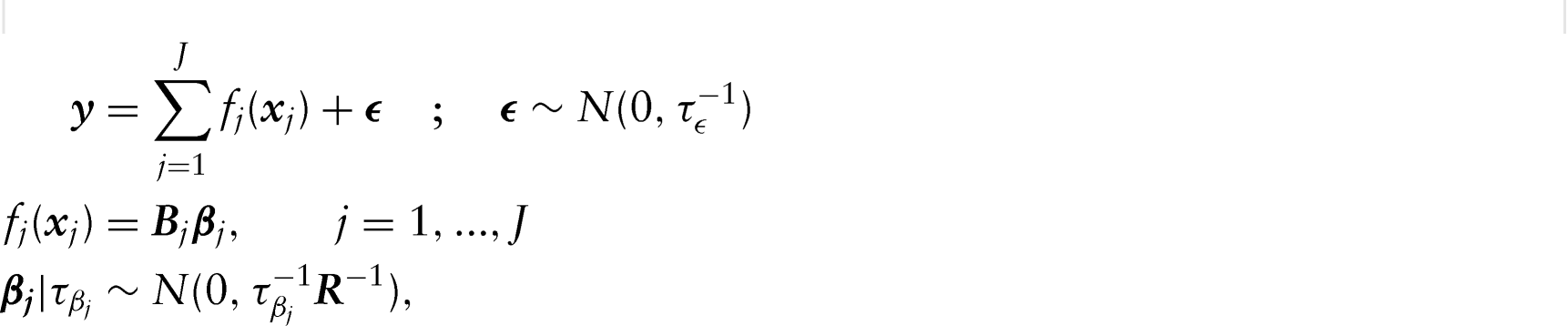
Let be observations of a response variable, be a continuous covariate, be a smooth function describing the effect of the covariate on the response and be independent errors with zero mean and variance . The P-spline model (Eilers and Marx, 1996) is , , where is a basis matrix containing B-spline functions built on a set of equally spaced (for simplicity) knots within the covariate domain, while is a vector of unknown spline coefficients. The method requires to select a generous number of knots to over fit the data and then add a penalty on which smoothes adjacent spline coefficients. In the frequentist approach, is estimated via penalized maximum likelihood, conditional on a tuning parameter regulating the degree of smoothness of . The optimal tuning can be found via cross-validation (Wood, 2006) or estimated via restricted maximum likelihood in a mixed model representation (Ruppert et al., 2003 chapter 4). P-splines are widely used in generalized additive models (Hastie and Tibshirani, 1990; Wood, 2006) or structured additive regression models (Fahrmeir et al., 2004; 2013). Higher dimensional smooth functions can also be represented as P-splines, using the tensor product of marginal B-spline bases (Currie et al., 2006; Eilers et al., 2006). For a systematic presentation of the different approaches to p-spline regression, see Ruppert et al. (2003); for an excellent review of spline methods and their applications in statistical modelling, see Hastie et al. (2009), Wakefield (2013) and Wood (2006).
Bayesian P-splines
The Bayesian approach to P-splines (Lang and Brezger, 2004) assumes an IGMRF prior on the spline coefficients,
where the precision is given by . Matrix is denoted as the structure of the IGMRF, that is, a sparse matrix with non-zero entries indicating conditional dependencies among the spline coefficients, is a scalar precision hyper-parameter and is the generalized determinant. Throughout the article, we will assume , where is a matrix such that (Eilers et al., 2006), with the -order difference operator. In this form, is the structure of an -order random walk on (Rue and Held, 2005 Chapter 3), with , where indicates the order of the IGMRF (2.1).
The IGMRF (2.1) describes deviation from a base model, which is a polynomial of degree . The amount of deviation depends on . A fully Bayesian specification requires priors on and . Since we usually have enough information in the data to estimate , the prior has less impact on the fit. The hyper-parameter enters at a lower level in the hierarchy, the data bring little information on it and the prior can have a substantial impact on the posterior distribution of and, as a consequence, on the smoothness of . Therefore, specification of should be as consistent as possible with the prior information actually available about the smoothness of the function to be estimated.
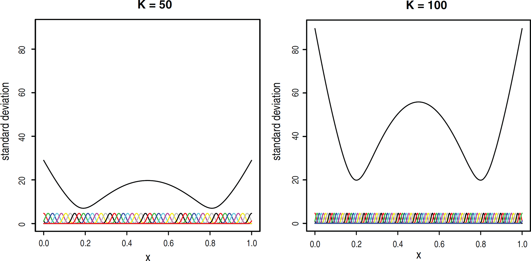
The marginal variance of the IGMRF (2.1), given by the diagonal elements of the generalized inverse matrix , depends on . We denote this as the ‘scaling issue’ (Sørbye and Rue, 2014), meaning that the amount of deviation from the base model depends on the number of knots. This is illustrated in Figure 1, where the two panels report the marginal standard deviation of the smooth , for . On the other hand, results (not shown here) show that the degree of the B-splines has little or no impact on the marginal variance of , especially when is large enough, say .
Degrees of freedom
The scaling issue can be avoided if we consider building priors on the number of effective degrees of freedom (Hastie and Tibshirani, 1990), . If we think of the smooth as a polynomial, then can be thought of as the degree of this polynomial. In presence of prior information on the degree of an equivalent polynomial, it seems to be a sensible approach to design a prior for , , instead of .
A fundamental issue when building is that depends on both precisions and . The former regulates the number of effective degrees of freedom, conditionally on the latter. When is known, the construction of can be based on the prior (see Section 4). When is unknown, the prior will be specified in terms of the joint , following a fully Bayesian approach (see Section 5).
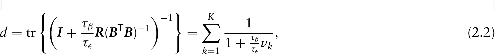
The degrees of freedom can be reduced to
where are the eigenvalues of , whose null space has dimension (the rank deficiency of ). When the factor goes to infinity, we obtain the minimum number of degrees of freedom, . When goes to zero, we obtain the maximum number of degrees of freedom, , corresponding to the most flexible model under the assumed IGMRF.
The prior depends on the eigenvalues of , hence on the choice of . Hereafter, will be referred to simply as ‘design’, because it is determined by both the assumptions made by the user (location and number of knots, order of the B-splines) and the assumptions purely made by design (location and number of observations along the covariate domain). Since the degrees of freedom depend on , it follows that automatically accounts for the design. This will be discussed in detail in Section 4.2.
The scaling issue. The two panels show the marginal standard deviation of for varying dimension of the basis , , where is a matrix of cubic B-splines (coloured lines) defined over the interval and is an IGMRF of order 2. The standard deviation (black line) is calculated as the squared root diagonal entries of , with .
PC priors for P-splines
The PC prior framework by Simpson et al. (2014) introduces a new concept for building priors in hierarchical additive models, where the latent structure is given by the sum of a number of model components described by a small number of flexibility parameters. Each model component is seen as a flexible extension of a base model. For instance, is a flexibility parameter for the IGMRF component and a natural base model corresponds to . Below, the four principles underpinning the construction of a PC prior for are reviewed, following Simpson et al. (2014).
Parsimony: A simple model should be preferred unless there is enough evidence for a more flexible one. Under this principle, the prior probability mass assigned to models of increasing complexity should decay as their distance from the base model (measured in terms of model complexity) increases. In Bayesian P-splines, the IGMRF prior operates on (the object of inference), but we can extend the notion of base and flexible model to the ‘spline-modelled’ function; we denote with the base model, which is a polynomial of degree , and with the flexible model, which reflects any deviation from such polynomial.
Measure of complexity: The Kullback–Leibler divergence (Kullback and Leibler, 1951) is assumed to evaluate the distance, , between the complexities of two different models. We use to denote the increased complexity of the flexible model with respect to the base model . Since is fixed by design, it is enough to evaluate . Let and be the precisions of the base and flexible models, respectively; it can be shown that goes to , for much lower than and ; see a proof in Simpson et al. (2014). Finally, for convenience we take the transformation .
Constant rate penalization: Flexible models are penalized by a constant decay rate for increasing . Following this principle, the PC prior is defined as an exponential distribution on the distance scale, , with constant rate . It follows that the mode of a PC prior is always at the base model. By a change of variable and setting the rate , Simpson et al. (2014) obtain the PC prior for as,
which is a type 2 distribution, .
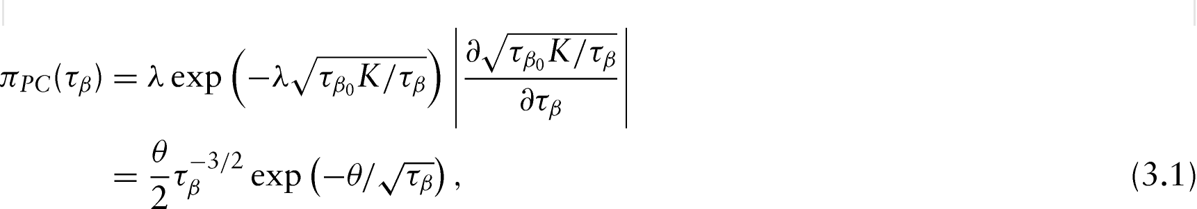
User-defined scaling: Often, the user has an idea about the size of an interpretable transformation of the original parameter , say (e.g., degrees of freedom). In this case, the user may elicit an upper bound for and set a prior probability for the tail event, that is, . Simpson et al. (2014) suggest to bound the marginal standard deviation, . To obtain in equation (3.1), it is enough to specify and solve for , which yields .
PC priors can be helpful as ‘default’ priors in complex hierarchical models where, typically, ‘it is difficult to elicit information about structural parameters that are further down the model hierarchy’(Simpson et al., 2014). In addition, the user-defined scaling approach enables to build ‘informative’ priors for the original parameter or for a property of the associated model component, by tuning two intuitive parameters and . In the next section, we introduce a new scaling approach to derive the PC prior for the degrees of freedom of a P-spline model component . Other approaches might be possible though. For instance, recently Klein and Kneib (2015) proposed PC priors for the scale (or range of variation) of and showed via simulation that these outperformed the gamma family in cases where the data are weakly informative and/or the size of the effects is close to the base model.
PC priors for degrees of freedom
A new scaling approach
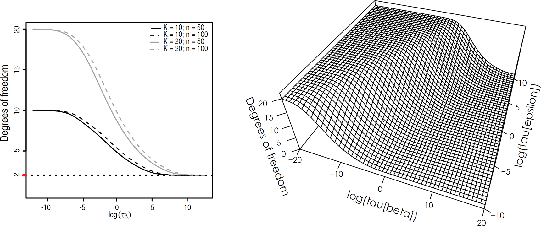
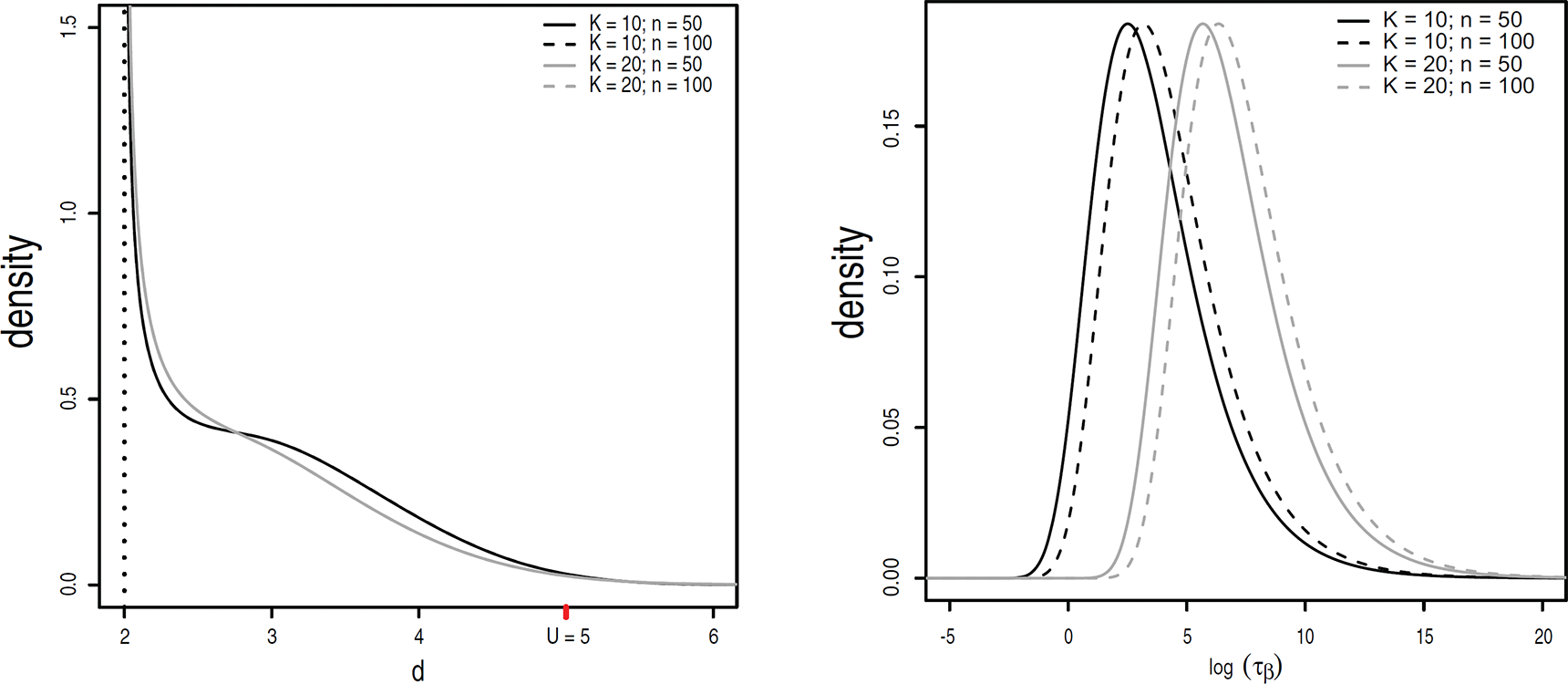
With no loss of generality, we derive the PC prior for degrees of freedom and study its properties under the assumption that the noise precision is known. Given , denote as the function mapping the precision into the number of effective degrees of freedom, following equation (2.2). (Hereafter, will be referred to as the mapping). Figure 2 shows the mapping in the log precision scale for and various designs (left panel) and for a specific design and varying (right panel).
We introduce a new user-defined scaling operating not directly on but on . Let be an upper bound for and a (small) probability associated to the tail event,
where is the cumulative distribution function (c.d.f.) of the type 2 distribution. The PC prior resulting from this new scaling is a Gumbel type 2 as in equation (3.1) with . In the following text, will denote the ‘induced PC prior for degrees of freedom’, with and the parameters specifying the distribution.
Invariance under design
While the PC prior for in equation (3.1) does not take into account any information regarding the adopted design, the induced PC prior for does. Indeed, different designs return different mappings (see the left panel in Figure 2), which implies a desirable property: the PC prior is ‘invariant under design’; the term invariant here applies to the interpretation of the PC prior in terms of degrees of freedom, not to the density. Figure 3 illustrates this property. The density of , with parameters , is displayed both in the scale (left panel) and scale (right panel), for different designs. By changing the design, the range of also changes and the density adapts accordingly (Figure 3, left panel). However, even if materializes differently in different designs, the probability mass assigned to is always . In the scale, the location of the PC prior is shifted between different designs (Figure 3, right panel). In our opinion, this shows well how difficult it is to define priors for degrees of freedom in the original scale: In this case, the user would have to figure out the correct location of and shift it according to the adopted design.
Mapping the degrees of freedom. The plot on the left shows the mapping in the scale, conditional on , for four designs (choices of and ). The dotted horizontal line at indicates the base model (assuming an IGMRF of order 2 on the spline coefficients). The plot on the right shows as a function of both and , for the specific design .
The PC prior plotted in the left panel of Figure 3 has been obtained numerically. Let be the PC prior equation (3.1) evaluated at some predefined (a convenient approach is to take on a regular grid inside ) and be the associated degrees of freedom computed by equation (2.2). The induced PC prior evaluated at is .
Invariance under design. Both panels show the PC prior density , for and , in two different scales: (left panel) and (right panel). In the left panel, the dotted vertical line at indicates the base model (assuming an IGMRF of order 2 on ), while the red tick indicates the upper bound () for degrees of freedom. Even if the PC prior density changes for varying and , the probability assigned to is always . In this particular example, the density change between and is evident in the scale (right panel), but not in the scale (left panel), where the solid and dashed lines appear superimposed (however, they are not the same because the eigenvalues of are different).
Behaviour near the base model
According to Simpson et al. (2014), the prior , where is the distance from the base model, is said to overfit, or to force overfitting, if . Theorem 1 in Simpson et al. (2014) states that if is an absolutely continuous prior for the IGMRF precision , with , this prior overfits. The commonly used , , with falls in this class of overfitting priors.
PC priors avoid over fitting by construction: By applying the first three principles outlined in Section 3, the mode of a PC prior is always at the base model. The fourth principle essentially allows the user to specify the penalty for increasing distances from the base model. The following result describes the behaviour near the base model for both the PC priors for degrees of freedom and the distribution of the degrees of freedom induced by a on , which we denote as . (In the result below, we consider , where is the mapping given a positive and finite .)
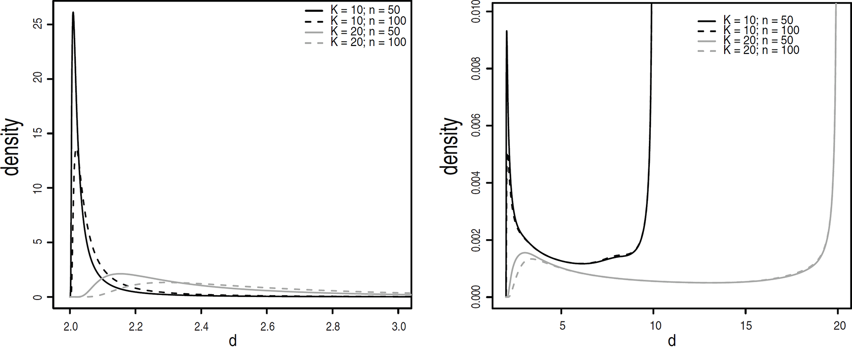
Result: Let be the dimension of the null space of in equation (2.1), then as , for , and as , for .
The proof is given in Appendix 9. The density goes to infinity as approaching the base model, avoiding over fitting. Instead, the gamma-induced does not prevent over fitting as it repulses the base model. In Figure 4, the gamma-induced priors with (left panel) and (right panel) are displayed under four different designs. These two different priors have different interpretations in terms of degrees of freedom: the first favours over-smoothing, while the latter favours over fitting. For both choices of and , the base model is repulsed at a different rate according to design. Indeed, for and fixed, the density clearly changes with design: In general, gamma priors are not invariant under design as a consequence of the scaling issue discussed in Section 2.1.
The distribution of the number of effective degrees of freedom induced by a gamma prior with (left panel) and (right panel), under four different designs. The base model is at , assuming an IGMRF prior of order 2 on .
P-splines with a joint prior on
So far we have worked under the assumption of known noise precision . The number of effective degrees of freedom is a function of , which scales differently according to the level of noise present in the data (see the right panel in Figure 2). Knowing is then crucial to scale the PC prior correctly, in order to guarantee the upper bound for degrees of freedom specified by the user.
The noise precision is typically unknown in applications. One could estimate from the data and then specify the PC prior for conditional on this estimate; this strategy has been proposed by Fong et al. (2010) to define gamma-induced priors for degrees of freedom. We, instead, adopt a fully Bayesian model,
where equations (5.3) and (5.4) specify a joint prior . The scaling parameter in equations (5.3) is given by , where is the mapping conditional on the random noise precision . We use the improper since the data usually contain sufficient information with respect to . The joint prior in equations (5.3) and (5.4) corresponds to the induced PC prior for conditional on a random , with and the parameters specifying the distribution.
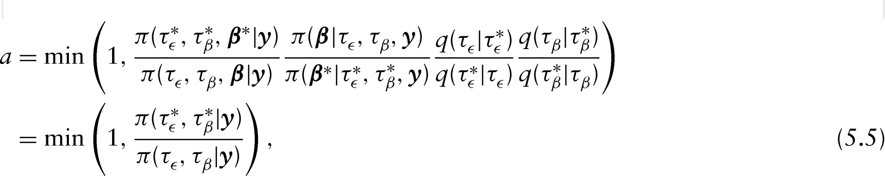
We developed a Markov chain Monte Carlo (MCMC) algorithm to fit the model in equations (5.1)–(5.4); see pseudo-code reported in Appendix A.2 algorithm 1. The algorithm includes a Metropolis–Hastings step to jointly update . In our experience, block updating ensures good mixing and fast convergence of the proposed MCMC algorithms; see Rue and Held (2005) for details on block updating in hierarchical models with GMRF components. A brief description on how algorithm 1 works follows. At iteration , both precision parameters (here denoted simply as ) are sampled from the proposal distribution adopted in Knorr-Held and Rue (2002): , where and are, respectively, the proposed and current values at iteration , is random with density , for and is a tuning parameter; in our experience, setting approximately equal to works well in most applications. The proposal has the advantage that the ratio equals one; for more details on this, see Rue and Held (2005), Chapter 4.2. Given and , we draw from the full conditional . Within this scheme, the acceptance probability for simplifies to (dropping the superscript to ease the notation)
where Computing the acceptance probability in equation (5.5) only requires the marginal for the precision parameters evaluated at the proposed and current values. Note that rescaling according to the proposed is needed before accepting/rejecting ; this implies re-evaluating the inverse mapping , given , and recomputing at each iteration.
Additive P-splines
We now focus on an additive P-spline modelling framework, where the linear predictor is the sum of a number of smooth functions. Let be a Gaussian response and , , be a set of continuous covariates; the model is
where is the B-spline basis matrix and the vector of spline coefficients associated to the smooth function ; with no loss of generality, we consider the same number of knots , yielding , . We assume the joint prior , where and , . The scaling parameter , where are the parameters calibrating the induced PC prior for the degrees of freedom of . The mapping for the degrees of freedom of is given by .
Identifiability constraints are important in additive P-splines. The IGMRF prior on controls deviations of the smooth term from a polynomial base model; in the following, for simplicity, we consider an IGMRF of order 2 (which forces shrinkage towards a linear base model). All smooths include the linear base model, thus they all compete to capture the mean of the data. To ensure identifiability, we adopt the following reparametrization,
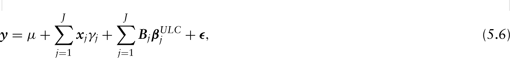
where is the intercept, is the slope coefficient for covariate and are the spline coefficients under the two following linear constraints: and , with ‘constant’ vector and ‘line’ vector . In this way, the smooth term captures residual variations from the linear base model . In other words, the constrained model (5.6) allows each smooth component to be identified, by separating the linear and flexible terms which coexist in each . Model (5.6) can be expressed in compact form as
where is the joint basis matrix, is the joint vector of spline coefficients subject to the linear constraints, is the matrix of covariates with an additional column of ones for the intercept term and is the vector of fixed effects. We assume with a small precision, for example, , as a prior for the fixed effects. Other covariates can be added to in model (5.7), if we assume them to have a simple linear effect.
We wrote a block updating MCMC algorithm implementing the joint prior in the model described above; pseudo-code is given in Appendix A.2 algorithm 2. This includes Metropolis–Hastings steps to jointly update the blocks and , for each ; in our experience, this scheme gives good mixing (and convergence) properties. Algorithm 2 presents two main changes with respect to algorithm 1. First, rescaling the conditional PC prior is no longer necessary at each iteration; must be recomputed only when is accepted. Second, the spline coefficients are sampled under linear constraints. To do this, we use the algorithm proposed in Rue and Held (2005), Chapter 2, which samples first the unconstrained coefficients and then ‘corrects’ them for the constraints. To compute the acceptance probability for the candidate in step (14) of algorithm 2, Appendix 10, the full conditional density is evaluated at the constrained ; for computational details, see Rue and Held (2005), formula 2.31.
Simulation study
The scaling parameter of the PC prior equation (3.1) can be tuned in several ways. Our proposal is to select through assumptions on the number of effective degrees of freedom, , of the function . This approach seems intuitive in the Gaussian case where quantity relates immediately to the degree of an equivalent polynomial (which an expert user might have prior information about). Moreover, literature on smoothing often refers to degrees of freedom as a way to summarize model complexity. In a recent paper, Klein and Kneib (2015) specify through assumptions on the ‘scale’, or range of variation, of and denote this PC prior as ‘scale-dependent prior’ (SD prior). Precisely, is derived numerically by requiring that for each in the covariate domain, where and indicates an upper bound for the scale of . Both scaling approaches lead to a PC prior which is invariant under design, in the sense that the computation of accounts for the adopted B-spline design . However, the two PC priors differ regarding conditioning on the noise variance. Our PC prior, , is a joint prior , while the SD prior is defined unconditionally on as the scale of does not depend on .
In this section, we present a simulation study which investigates further the relevance of degrees of freedom for designing priors for Gaussian P-splines. The objective of our study is to assess the behaviour of our joint prior in scenarios with different noise levels, and to compare this with two alternative priors which are defined unconditionally on , namely the conjugate gamma prior and the SD prior. Therefore, our simulation study does not aim to generically assess the behaviour of PC priors compared to standard priors. For an extended simulation study evaluating the performance of PC priors (particularly SD priors) compared to several alternative hyper-priors for variance parameters, in both Gaussian and non-gaussian contexts, the reader is referred to Klein and Kneib (2015). Furthermore, our simulation is restricted to the Gaussian case.
We consider two different models regarding the shape of the true :
Model is close to the base model (almost a linear effect; this is the same model considered in Klein and Kneib, 2015), while is a one-cycle sinusoidal curve (highly non-linear effect). In both scenarios, data are simulated as , where covariate takes values on a regular grid. We assume a standard P-spline model with one covariate, , , where is the structure of an IGMRF of order 2, and contains cubic B-splines evaluated at .
Different scenarios are generated by setting: (small and moderate sample sizes), , (high, moderate and low noise). We aim to assess the model fit obtained by the following priors:
conjugate gamma prior on , with two specifications widely used in applications: and .
our joint prior , inducing a PC prior for degrees of freedom, , with parameters and . We set and various upper bounds . Note that we specify only to check consistency of results in the limit case where any deviation from the base model is strongly penalized (in applications, this is not a sensible choice as it forces the fit towards a linear trend; for more details, see the joint prior in action with simulated data in the supplemental material).
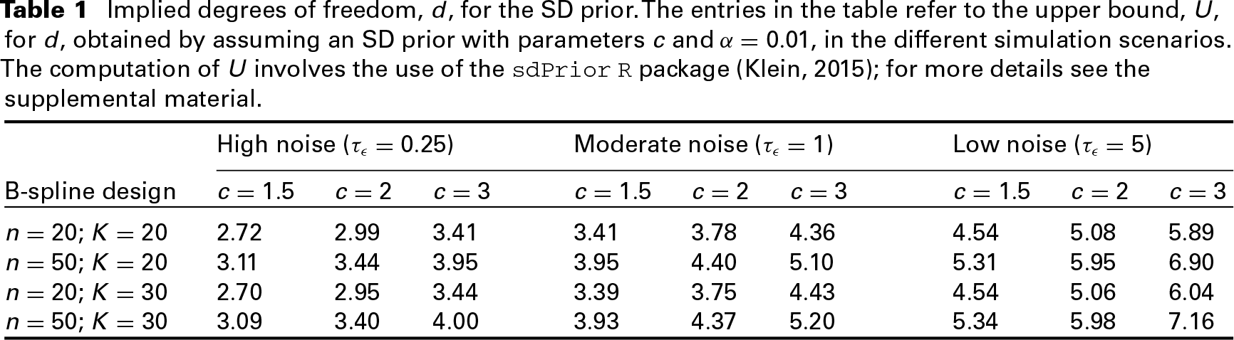
SD prior on (Klein and Kneib (2015)), with and three specifications for the scale of , . Note that since both and vary within , seems the most sensible choice as an upper bound for the scale of both functions, resulting in a sufficiently flexible prior, while leads to an even more flexible prior. However, from Table 1, we see that the degrees of freedom implied by an SD prior with parameter strongly depend on the noise present in the data (and to some extent on the adopted design): for instance, implies an upper bound for around in the high noise case (for the design , ) which results into a very restrictive prior in fact.
Implied degrees of freedom, , for the SD prior. The entries in the table refer to the upper bound, , for , obtained by assuming an SD prior with parameters and , in the different simulation scenarios. The computation of involves the use of the sdPriorR package (Klein, 2015); for more details see the supplemental material.
High noise ()
Moderate noise ()
Low noise ()
B-spline design
;
;
;
;
Results
In each scenario, goodness of fit was assessed for each of 1 000 simulated datasets by the mean squared error (MSE) of , where is the posterior mean, as MSE . The posterior for was computed using R-INLA (Rue et al., 2009, www.r-inla.org) for the gamma and SD priors, and using MCMC algorithm 1 for the joint prior. For the sake of comparison between the three classes of priors, we assume throughout the simulation study (hence, our joint prior is ).
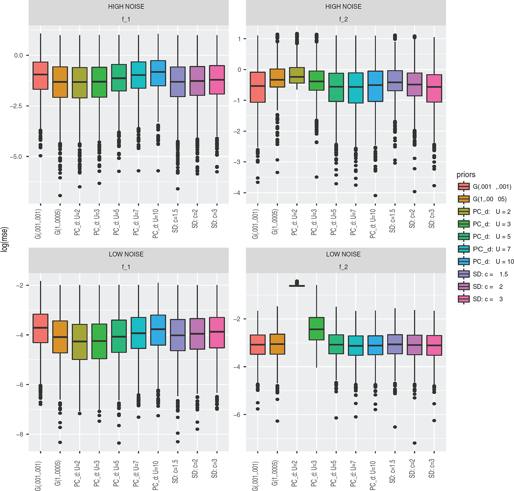
Figure 5 reports for small sample size (which is when the hyper-prior is expected to be most influential on the posterior) and . We do not see much change for increasing and , thus results for other scenarios are only reported in the supplemental material. Our main findings are as follows:
The gamma priors are generally outperformed by the two PC priors (both for degrees of freedom and scale), unless the data are very informative about the true model (e.g., in model with low noise, see bottom-right panel in Figure 5). As expected, the overfits when model is the true one (see left panels in Figure 5), while the performs poorly in scenario (especially with high noise, see top-right panel in Figure 5).
For sensible choices of the upper bound , the joint prior performs better than, or at least as good as, the SD prior. The main difference is noticed in scenario with high noise (top-right panel in Figure 5) and scenario with low noise (bottom-left panel in Figure 5). In the former case, setting the joint prior with outperforms most SD prior specifications; in particular, the SD prior with achieves poor performance because the implied upper bound for is too small (i.e., below , see Table 1) for this case, where the true effect is highly non-linear and the data are very noisy. The SD prior with gives similar performance because it implies a larger upper bound for degrees of freedom. Instead, in scenario with low noise, SD priors are outperformed by the joint prior with , because any choice implies an upper bound for clearly larger than needed (i.e., above , see Table 1) in this case, where data are very informative and the true effect is close to the base model.
In cases where the choice of the upper bound is inappropriate to describe the complexity of the true function , the joint prior performs poorly. For instance, when the true curve is close to the base model (i.e., scenario ), the joint prior with is outperformed by both the SD priors and the (see left panels in Figure 5); in other words, when data are generated under a linear model, a joint prior with large upper bound will result in a bad choice, as it allows ‘far more’ degrees of freedom than needed. For the same reasons, when the true curve is highly non-linear (i.e., scenario ), the joint prior with generally achieves poor performance (see the right panels in Figure 5), because it assigns almost all weight to the base model or close to it.
In summary, the simulation study showed that both PC priors (i.e., the SD prior and our joint prior) provide potentially better performance than the standard gamma priors for sensible choices of the scaling parameter . None of these PC priors shows uniformly better performance than the other one. However, we think that the particular scaling approach used to tune plays an important role. Scaling the PC prior in terms of degrees of freedom automatically accounts for the level of noise present in the data. We were able to show via simulation that our joint prior has the potential to perform well in general, that is, both in high and low noise cases, provided that the elicited is an appropriate upper bound for the degrees of freedom of the function underlying the data. Therefore, we conclude that the number of effective degrees of freedom is a relevant quantity for building PC priors for smoothing Gaussian data, more suitable than other transformations of that do not depend on .
Simulation results: for (left panels) and (right panels), in presence of high noise (, top panels) and low noise (, bottom panels), sample size , . In the legend on the right, label ‘G’ indicates the Gamma prior; ‘PC_d’ indicates our PC prior for degrees of freedom (joint prior), with and ; ‘SD’ denotes scale dependent prior with and .
Application
We demonstrate the use of the joint prior within an additive P-spline framework for modelling nitrate concentration in river Oglio, Lombardy, Italy. A total of observations of NO concentration were collected during 2010–2012 by taking one sample at each season (spring, summer, autumn and winter) in 48 gauging stations located along the river catchment. The response variable is , measured at station and season . Covariate streami is the distance from each station to the Iseo lake (i.e., the river source) measured in km along the stream network; the first station in proximity to the lake is at , while the last station downstream the river is at . The goal is to understand ‘river enrichment’ in terms of nitrates, by studying the behaviour of as the stream distance increases. A substantial amount of information comes from previous studies (see Bartoli et al., 2012; Delconte et al., 2014 and references therein), suggesting that river enrichment in terms of nitrates may vary non-linearly as the stream distance increases. Due to different characteristics in terms of groundwater interactions and irrigation practices, the river catchment can be divided into upstream, middle and downstream reach. Different processes are expected within the three reaches and between seasons; hence, the enrichment curve may show different shapes in the three river segments and seasons.
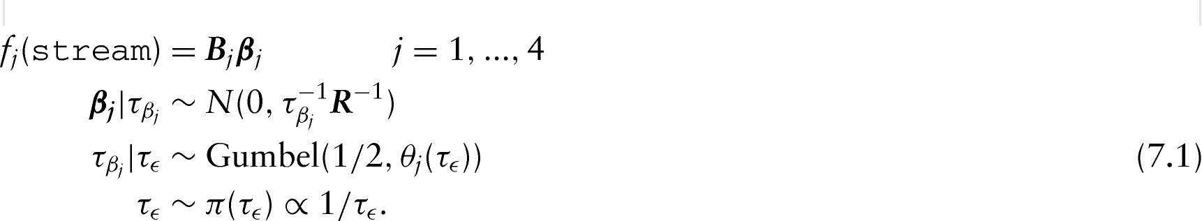
In order to investigate possible seasonal effects on river enrichment, we adopt the model: , , , where is the overall intercept, is the season-specific intercept and is the season-specific smooth function of the stream distance, modelled with a P-spline with joint prior on as described in Section 5,
We assume an IGMRF of order 2 with precision on each . Based on our prior information, we specify an upper bound for the PC prior equation (7.1), for all , assuming that each is much more flexible than linear (i.e., ) and assigning two additional degrees of freedom to each of the three river segments, to capture possibly different enrichment behaviours. We believe that this prior is flexible enough to describe the possible smooth change between the upstream middle and downstream behaviours. We set , saying that it is likely that is more flexible than eight degrees of freedom, .
To construct the matrices and of model (5.5), we need to create suitable dummy vectors of length : , , taking value 1 when the observation is from season and 0 elsewhere (these are associated to the season-specific intercepts); , , taking the actual stream distance when the observation is from season and 0 elsewhere (these are associated to the season-specific slopes). The fixed effect design matrix is , with and . Each basis contains cubic B-splines, evaluated on the season-specific stream distances . The B-spline design matrix is . To separate the season-specific slopes and intercepts from the season-specific smooth variation captured by the B-splines, suitable linear constraints must be applied to each , as discussed in Section 5.1. We fit this model via MCMC based on the pseudo-code reported in Appendix A.2 algorithm 2; in particular, we use a two blocks-updating scheme, which ensured good mixing: first block is and the other one contains all the four sets of spline coefficients and associated precisions, . During MCMC iterations, the PC prior for each precision needs to be rescaled according to the current , but this can be done at a negligible computational cost. The R code is provided as supplemental material.
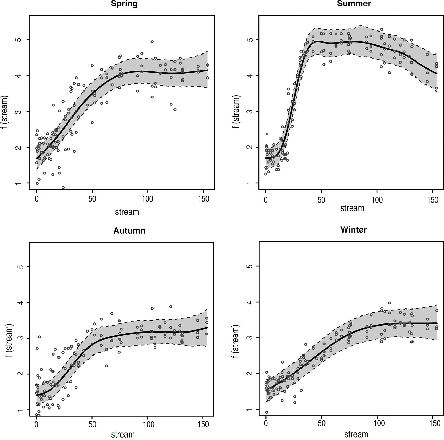
The results displayed in Figure 6 reveal different river enrichment curves () in different seasons: A distinctive pattern is observed in summer, where the fitted curve shows a fast increase upstream ( km) and tendency to decrease downstream the river ( km). This pattern supports the argument given in Delconte et al. (2014) about an upstream reach (from 0 to 25 km) where nitrates are stable, reflecting the chemistry of the lake; a middle reach (from 25 to 80 km) showing an increase of NO concentration, probably due to groundwater inputs as replacement of river water abstracted for irrigation; a downstream reach (from 80 to 150 km) where nitrates should remain constant or even decrease, mainly due to the dilution of river water with NO-deprived inputs.
Estimated river enrichment curves (, black line), for each season, and credible bands (grey). The curve for summer shows clearly a distinctive pattern with respect to the other seasons. Partial residuals (Wood, 2006) are plotted in each panel (dots), indicating larger variability, than what assumed by the model, for the log NO concentrations observed in spring and autumn (with possible outliers in the upstream river segment in autumn).
Discussion
PC priors are defined to penalize complexity with respect to a given base model, the magnitude of the penalty being elicited by the user using an intuitive scaling approach. The scaling tool allows the user to derive the PC prior on an interpretable scale, different from the scale of the original parameter, provided that the link between the two is known. We took advantage of this nice feature and derived PC priors for the number of effective degrees of freedom of a P-spline model for Gaussian data.
For non-Gaussian responses, the idea presented in this article follows straightforwardly by assuming the definition of the degrees of freedom of a generalized P-spline model (Hastie and Tibshirani, 1990), , where is a diagonal matrix, with entries depending on the linear predictor of the model (i.e., on ) and the adopted link function. MCMC methods similar to those proposed in this article can then be developed being careful about implementing the mapping , which is conditional on in the generalized case (note that for most distributions in the exponential family, is known, e.g., for Poisson we have ). For Poisson and binomial responses, a convenient approach is to use auxiliary variable methods (Frühwirth-Schnatter and Frühwirth, 2007; Frühwirth-Schnatter et al., 2008) and work with an equivalent ‘augmented’ P-spline model for Gaussian (pseudo) data. The PC prior for can then be implemented in the same way as described in this article, with algorithms 1 and 2 needing only the inclusion of a Gibbs step to update the augmented parameters.
The potential advantages of using PC priors for degrees of freedom are twofold. First, they are ‘easy-to-elicit’ by the user, who has to define two intuitive scaling parameters: , an upper bound for , and , the prior mass assigned to . This scaling tool can be handled flexibly. For instance, elicitation of the median for the degrees of freedom results from fixing . In this case, the PC prior density is bimodal: one mode is set at the base model (by definition) and another mode is set around degrees of freedom. This bimodal behaviour is due to the attraction to the base model implicit in PC priors.
As a second advantage, these PC priors avoid overfitting and are invariant under design, which means that the parameters and do not need to be rescaled if the design changes. In other words, the PC prior is able to code into the model the prior knowledge on the complexity of the curve, or its degrees of freedom, in a design-adaptive way. The ability to adapt to design and avoid overfitting by construction makes an appealing default choice in additive models where the latent structure includes several smooth functions (built on a basis of B-splines, e.g., P-splines) and other types of structures, such as individual, spatial and spatio-temporal random effects.
Footnotes
Acknowledgments
Massimo Ventrucci is funded by a FIRB 2012 grant (project no. RBFR12URQJ, title: Statistical modeling of environmental phenomena: Pollution, meteorology, health and their interactions) for research projects of national interest provided by the Italian Ministry of Education, Universities and Research. The dataset used in Section 7 was kindly provided by the Consorzio dell'Oglio, from the project ‘Experimental assessment of the environmental flow in the lower Oglio river’. We thank Erica Racchetti and Alex Laini, Department of Life Science, University of Parma, for introducing us to the application in Section 7 and for fruitful discussion on the ecological interpretation of results. Finally, we would like to thank the Associate Editor and two anonymous referees for their helpful comments.
Appendices
References
1.
BartoliMRacchettiEDelconteCASacchiESoanaELainiALonghiDViaroliP (2012) Nitrogen balance and fate in a heavily impacted watershed (Oglio River, Northern Italy): In quest of the missing sources and sinks. Biogeosciences, 9, 361–373. doi: 10.5194/bg-9-361-2012. URL http://www.biogeosciences.net/9/361/2012/ (last accessed 28 July 2016).
CurrieIDurbánMEilersP (2006) Generalized linear array models with applications to multidimensional smoothing. Journal of Royal Statistical Society, Series B68, 259–280.
FahrmeirLKneibT (2009) Propriety of posteriors in structured additive regression models: Theory and empirical evidence. Journal of Statistical Planning and Inference, 139, 843–859.
9.
FahrmeirLKneibTLangS (2004) Penalized structured additive regression for space-time data: A Bayesian perspective. Statistica Sinica, 14, 715–745.
10.
FahrmeirLKneibTLangSMarxB (2013) Regression: models, methods and applications. Berlin: Springer-Verlag.
11.
FongYRueHWakefieldJ (2010) Bayesian inference for generalized linear mixed models. Biostatistics, 11, 397–412. doi: https://dx-doi-org.web.bisu.edu.cn/10.1093/biostatistics/kxp053. URL http://biostatistics.oxfordjournals.org/content/11/3/397.abstract (last accessed 28 July 2016).
Frühwirth-SchnatterSWagnerH (2011) Bayesian variable selection for random intercept modeling of Gaussian and nonGaussian data. In BernardoJMBayarriMJBergerJODawidAPHeckermanDSmithAFMWestM, eds. Bayesian Statistics9 pages 165–200, Oxford: Oxford University Press.
Knorr-HeldLRueH (2002) On block updating in Markov random field models for diasease mapping. Scandinavian Journal of Statistics, 29, 597–614.
23.
KullbackSLeiblerRA (1951) On information and sufficiency. The Annals of Mathematical Statistics, 22, 79–86.
24.
LangSBrezgerA (2004) Bayesian P-splines. Journal of Computational and Graphical Statistics, 13, 183–212.
25.
RueHHeldL (2005) Gaussian Markov Random Fields. London: Chapman and Hall/CRC.
26.
RueHMartinoSChopinN (2009) Approximate bayesian inference for latent Gaussian models using integrated nested laplace approximations (with discussion). Journal of the Royal Statistical Society, Series B, 71, 319–392.
27.
RuppertDWandPCarrollR (2003) Semiparametric Regression (Cambridge Series in Statistical and Probabilistic Mathematics). Cambridge, UK: Cambridge University Press.
28.
SimpsonDPRueHMartinsTGRieblerASørbyeSH (2014) Penalising model component complexity: A principled, practical approach to constructing priors. Statistical Science (published before print)URL http://arxiv.org/abs/1403.4630v4”arXiv:1403.4630v4 (last accessed 28 July 2016).