



Abstract
Highway safety improvement projects are identified by using either (i) a site-specific or (ii) a systemic approach. In the site-specific approach, locations for improvements are ranked according to different performance measures such as critical crash rate, expected crash rate or equivalent property damage only. Alternatively, in the systemic approach, roadway characteristics such as number of lanes, shoulder width, etc. are flagged as a ‘risk’ (or ‘preventative’) feature that increases (decreases) the risk of negative outcomes. Using the Highway Safety Information System database, we seek to merge the two approaches by, first, identifying roadway factors associated with an increased occurrence of car crashes (features we call ‘risk factors’) and, subsequently, identifying roadway segments with a higher crash risk. Specifically, we model the locations of crashes as a realization from a spatial point process. We then parameterize the associated intensity surface of this spatial point process as the sum of a regression on roadway characteristics and spatially correlated error terms. Thus, through the regression piece, we identify hazardous roadway features and through the spatially correlated error terms, we identify locations of high risk.
Introduction
Problem statement and data
The goal of highway safety improvement projects is to minimize the risk to users (drivers and pedestrians). Traditionally, improvement projects are identified by using either (i) a site-specific or (ii) a systemic approach. In the site-specific approach, locations for improvements are ranked according to different performance metrics such as critical crash rate, expected crash rate or equivalent property damage only (EPDO; Persaud et al., 1999; Heydecker and Wu, 2001). Alternatively, in the systemic approach, roadway characteristics such as number of lanes, shoulder width, etc. are flagged as a ‘risk’ (or ‘preventative’) feature that increases (decreases) the risk of negative outcomes (Knapp et al., 2014; Lord et al., 2007). Safety improvements are then made across the whole road system to decrease crash risk. Typically, systemic analyses rely on aggregating data to crash counts across similar roadways. However, each road segment has its own unique attributes based on the location of the roadway (e.g., off-road distractions) that may impact its risk level. In this way, spatial location of crashes may act as a confounding factor in systemic analyses.
For this research, we seek to merge the two approaches by both identifying roadway factors associated with an increased occurrence of car crashes (features we call ‘risk factors’) and identifying roadway segments with a higher crash risk. In this way, we seek to inform possible systemic safety improvements to the roadway system while accounting for spatial location which facilitates locating regions where improvements are needed. By combining the two approaches (site-specific and systemic) into one model, we account for the uniqueness in each road as we estimate the effects of the various roadway characteristics. This allows us to estimate the amount of total risk due to location, as well as estimate the risk due to roadway construction.
To accomplish these goals, this analysis seeks to model data from the Highway Safety Information System (HSIS; www.hsisinfo.org); a multistate roadway database overseen by the University of North Carolina Highway Safety Research Center. Currently, states participating in the HSIS include California, Illinois, Maine, Minnesota, North Carolina, Ohio and Washington. However, because of the differences in the variables from state to state (definition and availability), this research focuses on data from five interstate highways in Washington: Interstate 5 (I-5), Interstate 90 (I-90), Interstate 82 (I-82), Interstate 405 (I-405) and Interstate 705 (I-705). Figure 1 shows the locations of these roads (I-705, a 1.5-mile-long road connecting I-5 to Tacoma is not labelled on the map due to its small size). While we choose to focus on interstate highways in Washington here, we note that similar analyses can be performed for other states and roadway types.

The HSIS data include roadway inventory information (number of lanes, type of pavement, speed limit, traffic volume, etc.) and crash information (crash type, vehicle type, number of vehicles involved, etc.) for crashes that occur between the years 2010–2012. Because roadway characteristics vary slightly from year to year, we used roadway inventory data from 2012 to keep the roadway definitions temporally consistent. Given the short time span considered here (three years), the 2012 roadway characteristics are likely representative of the state of the roadway. Table 1 displays the variables used in this study, along with the associated HSIS database where the information was obtained.
Variables used in this study, and the associated HSIS database where the data was obtained

The response variable in the HSIS data considered here is the location of a crash, which we denote by
Kernel density estimates of crashes along each interstate highway considered in our analysis. Tick marks along the horizontal axis indicate exact crash locations. Vertical lines indicate the approximate centres of large cities along the interstate

Statistically speaking, the goal here is to, first, regress the road factors from Table 1 onto the observed crash locations to determine which characteristics are associated with the high levels (density) of crashes. Second, after accounting for the roadway factors, we seek to identify road segments that have a high risk for reasons not attributable to the roadway factors in the dataset. Thus, by accomplishing these two goals, we will not only identify possible systemic improvements to the highway system (risk factors) but also specific locations that could benefit from safety improvements.
There are two main challenges associated with these goals. First, as mentioned previously, the response variable is the location of the crash (interstate and mile marker). While regression is a simple goal, standard regression techniques such as linear or generalized linear models (Faraway, 2014, 2016) are not applicable for this type of response. One approach would be to aggregate (count) the number of crashes along predefined road segments. In doing so, models for count data such as zero-inflated Poisson (ZIP), negative binomial models or Poisson models may then be appropriate (Lord et al., 2005, 2007; El-Basyouny et al., 2014; Chiou and Fu, 2013), which can be implemented using either a frequentist or Bayesian paradigm (Schultz et al., 2011; Sacchi et al., 2015). Concerns with aggregating crash counts along predefined roadway segments include, first, the defined segments may be arbitrarily selected, second, information at the sub-segment level is forfeit and, third, it converts an inherent spatially continuous process into a discrete one.
Rather than aggregrating as suggested previously, we opt to treat the locations
Our research approach is to model
A second challenge in analysing the HSIS data is that the locations of crashes on road segments within a roadway network are spatially correlated. In other words, two locations on an interstate that are close together should have more similar crash rates than segments that are far from each other. In this spatial point process framework used here, this challenge translates to the need to model a smooth intensity surface in space. Work by Barua et al. (2015), Ahmed et al. (2011), Guo et al. (2010), Aguero-Valverde and Jovanis (2008, 2010) and Barua et al. (2014) suggest that including spatial correlation in the statistical model provides superior fit while providing unbiased estimates of model parameters. While methods for incorporating spatial correlation (smoothness) are well established (El-Basyouny et al., 2014), traditional spatial methods generally utilize straight-line distance to estimate the correlation between two points. Straight-line distance is certainly inappropriate for roadway networks because these networks do not allow for straight-line travel between any two points, but rather require travellers to use existing roads to get from point A to point B. As a solution, we incorporate spatial correlation into our model based on driving distance, rather than Euclidean distance.
To summarize, the primary contribution of this article is to simultaneously perform a site-specific and systemic analysis of the interstate network in Washington shown in Figure 1. In doing so, this article proposes a spatial point process model with appropriate regression terms and spatially correlated error structure. The remainder of this article is outlined as follows. Section 2 details the point process model and reviews relevant methodology from the literature. Section 3 presents results and interpretations, as well as assessing the model fit. Section 4 details our conclusions and plans for future work.
Model
Model details
As in Section 1.2, let 
In the point process framework, the intensity surface 
Let 

To intuitively understand the parameterization in (2.3), consider Figure 3 which shows a one dimensional intensity surface (solid curve) along with two resolutions of regions (two values of Two discrete approximations of continuous intensity surface (solid curve) using two different values for K. Horizontal line segments indicate maximum likelihood estimates of the surface and dashed lines indicate region boundaries
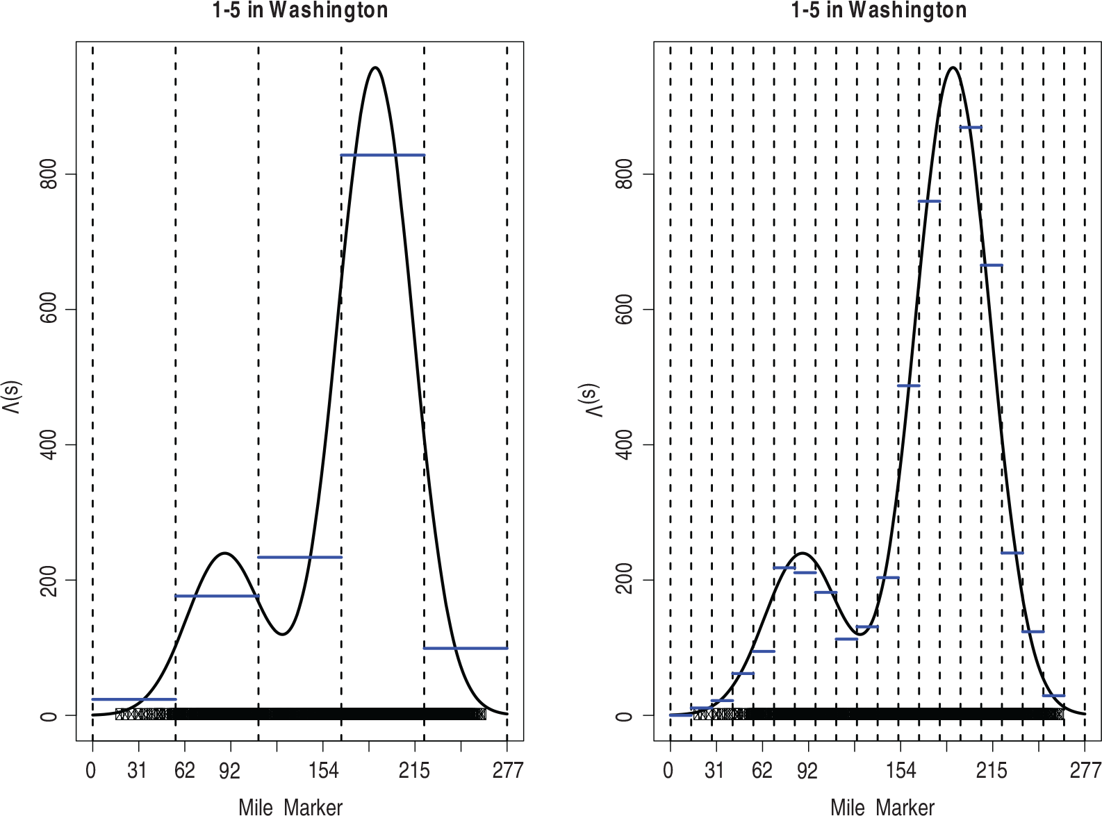
Intuitively, more crashes are expected in areas with higher traffic. However, since our first goal (see Section 1.2) is to identify roadway characteristics associated with a higher rate of crashes and safety improvement projects are not able to alter traffic levels, we factor


The
At this point, recall that our two goals are to, first, identify roadway features associated with high risk areas and, second, to identify ‘hot-spots’ where the crash risk is high after accounting for traffic and roadway features. These goals can be accomplished by regressing roadway features on 
The coefficients
The mean zero error terms
Marginalizing equation (2.7) over 
We opted to use the Bayesian paradigm (Gelman et al., 2014; Carlin and Louis, 2008) for parameter estimation, although we do note that parameter estimates can also be obtained via maximum likelihood. As prior distributions, we generally assumed vague priors, with a few exceptions which we detail here. First, we assumed
Theoretical work by Zhang (2004), Kaufman and Shaby (2013) show that estimation for
In order to estimate
Results
Using the draws from the posterior distribution, Figure 4 compares the observed crash counts on each road segment to the expected crash counts (defined as the posterior mean of
Comparison between actual crash counts for each 1-mile road segment in our data and expected crash counts for these same segments generated by our model. The extremely high correlation between the counts shows that our model fits our data.
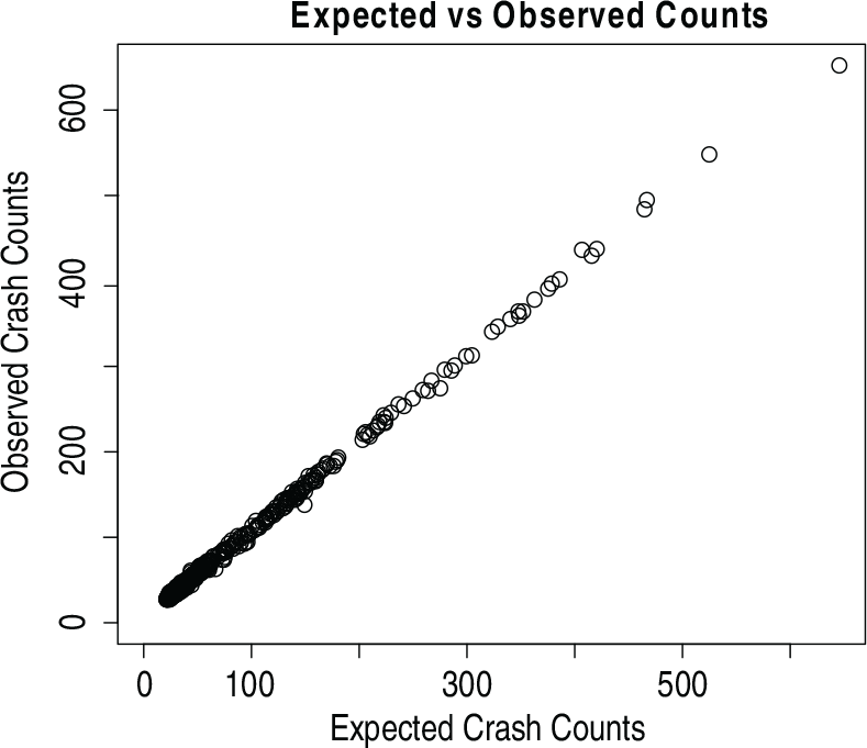
Comparison between actual crash counts for each 1-mile road segment in our data and expected crash counts for these same segments generated by our model. The extremely high correlation between the counts shows that our model fits our data.
Through our MCMC algorithm, we obtained draws from the posterior distributions for the effects of each of the roadway characteristics (i.e.,
The mean and 95% credible interval for the effect of each roadway characteristic and the probability of the magnitude of the effect being greater than 0. The type of variable is either quantitative (Q) or categorical (C)
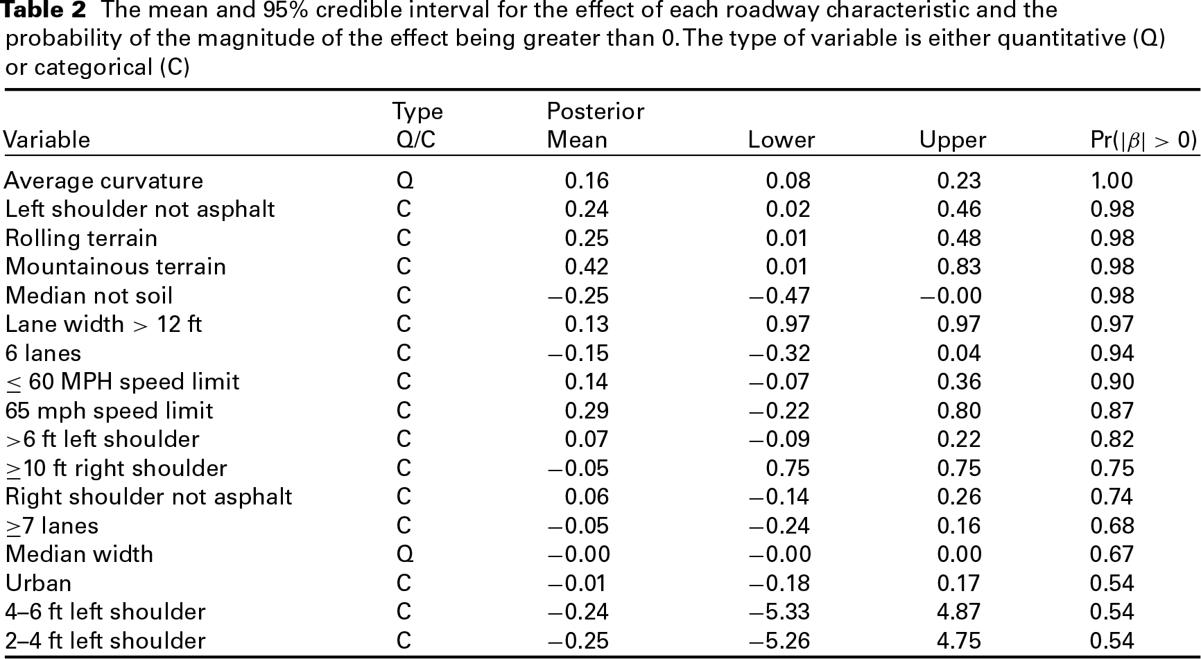
The mean and 95% credible interval for the effect of each roadway characteristic and the probability of the magnitude of the effect being greater than 0. The type of variable is either quantitative (Q) or categorical (C)
Consider, first, the quantitative variable ‘average curvature’ as an example. From Table 2, as the average curvature of a road segment increases by one degree, we would expect the log relative risk of the segment to increase by 0.16 (0.08, 0.23), on average. In other words, segments with higher average curvature tend to have a higher relative risk, or have more crashes than we expect given traffic volume. Conversely, because the posterior mean of the effect of median width is −9.3
The effects of the categorical variables speed limit, terrain type, median type, shoulder type, shoulder width, number of lanes, lane width and urban vs rural area are relative to the baseline categories which we chose based on the most common category observed in the data. Specifically, the baseline categories are a speed limit of 70 MPH, level terrain, soil median, asphalt shoulders, 0–2 ft left shoulder, smaller than 10 ft right shoulder, 5 or fewer lanes, 12 ft lane width and rural area type. As an example in how to interpret these effects, consider the effect of rolling terrain. Because the effect of rolling terrain is 0.25 (0.01, 0.48), road segments with rolling terrain tend to have a higher relative risk than those with level terrain. Conversely, because the effect of a median pavement type that is not soil is −0.25 (−0.47, −0.003), segments with non-soil medians (e.g., concrete or asphalt medians) tend to have a lower relative risk than those with soil medians.
Based on the results in Table 2, in terms of roadway construction, our recommendations would be to build straight, flat roads with asphalt left shoulders, medians of types other than soil (e.g., concrete medians), and lanes of 12 ft in width. Initially, it may seem surprising that speed limits lower than 70 MPH were estimated to increase the crash risk of road segment; however, we speculate that the high coefficients for the 65 and
As discussed in the Introduction, we seek to merge the site-specific and systemic approaches to highway safety analysis. The coefficients discussed previously highlight potential systemic improvements to the roadways. However, as discussed in Section 2, we expect that not all variability in the relative risk is explained by roadway characteristics; hence, we included the spatially correlated and independent error terms into our model specification (
This plot shows additional risk (not attributable to traffic levels or the roadway factors in our data) identified by our model for I-5 (left) and I-90 (right). The solid curves represent a kernel smoother of the residuals to highlight patterns

This plot shows additional risk (not attributable to traffic levels or the roadway factors in our data) identified by our model for I-5 (left) and I-90 (right). The solid curves represent a kernel smoother of the residuals to highlight patterns
Using the spatial residuals along I-5 in the left panel of Figure 5 as an example, we can see evidence of spatial clustering which, subsequently, justifies our use of spatial modelling. For example, notice that the residuals near Tacoma and Seattle are clustered above 0, indicating spatially related elevated risk for these areas that is not accounted for by our roadway characteristics. If not roadway characteristics, what contributes to the elevated risk in these areas? One possibility that we hypothesize accounts for these high residuals is driver distraction. Figure 6 displays a Google map image of miles 165–166 and 166–167 on I-5. Notice that there is a clear view of the Space Needle, a well-known Seattle landmark, along these road segments. This ‘off-road’ distraction, as well as other features in the major downtown area, could be a possible contributor to this added risk.
The view from mile 166 on I-5, obtained from Google Street View. The Space Needle, as well as other Seattle landmarks, is clearly visible from the road, which may distract drivers, possibly contributing to the increased risk in this area

Examining the right panel in Figure 5, there is a clear increase in risk for Seattle, a smaller increase near Spokane, and also a clear increase in additional risk from mile 50 to approximately mile 100. As displayed in Figure 7, a winter recreation resort, the Summit at Snoqualmie, is located at mile 51–53 and the Snoqualmie Pass, an occasionally hazardous mountain pass, is located at mile 54. The area is heavily forested and also includes other mountain recreation areas. We hypothesize that these factors may be associated with interstate entrance and exit ramps as well as further distractions for drivers. Furthermore, the highest peak in the residuals, within the mile 50 to mile 100 region of I-90, occurs at mile 86–87. This location is where I-90 crosses the Yakima River, another potential distraction to drivers.
Google Maps image of miles 50–54 on I-90, an area identified by our model as a region of high risk not attributable to the roadway factors in our data. A ski resort, the Summit at Snoqualmie, as well as other recreational areas, are located here suggesting that driver distraction and frequent interstate entrances and exits may contribute to risk

Finally, beyond systemic and site-specific approaches individually, our modelling strategy has the ability to merge these two approaches to estimate the overall risk
The posterior mean of the relative risk
over I-5 (left) and I-90 (right). If
, there were fewer crashes than expected due to traffic levels and if
there were more crashes than expected

Looking at Figure 8, recall that
In this article, we implemented a framework to use spatial statistical methods over a roadway network in order to identify factors associated with high crash counts (a systemic approach), as well as to pinpoint road segments of interest which had higher crash rates than expected (a site-specific approach). To do this, we assumed crash locations followed a non-homogeneous Poisson process. The intensity surface of the Poisson process was subsequently modelled as the sum of a regression piece (to estimate the impact of roadway features) as well as spatial and non-spatial residuals. Systemically, our results indicated that increasing the shoulder width, decreasing curvature and including a non-soil median (i.e., concrete barriers) decreases the overall crash risk. Likewise, our site-specific analysis suggests that distractions and frequent entrances and exits from the interstate contribute to increased crash risk. While our results are informative for highway safety improvement projects, we recommend that more research be done to determine the aspects of major metropolitan and recreational areas which increase the riskiness of roads.
We emphasize that our results here are associations rather than causal relationships. We do not have information on what caused these specific crashes (i.e., from police records). Rather, we merged roadway databases with crash databases to investigate trends in systemic features and roadway segments with crash locations. An interesting area of future research would be to investigate the use of causal methods for highway safety analyses and contrast our results with those of a causal analysis (Karwa et al., 2011).
For this analysis, we considered all crashes. However, we hypothesize that roadway features correlate differently for various types of crashes. For example, adding a concrete barrier could decrease the number of ‘run off the road’ crashes yet increase the number of ‘multiple vehicle crashes’ because cars, possibly, would veer into other lanes to avoid hitting the barrier. In the future, we plan to extend our methodology to account for the types of crashes in a multivariate framework. Additionally, this research only considered an interstate network. We are also interested in using this methodology to examine more complex roadway networks, possibly by including highways as well as interstates.
Another possible direction for future research would involve incorporating crash severities into the relative risk of road segments. For example, road segments with lower speed limits may observe a high number of total crashes but have a low average severity, while segments with higher speed limits may observe fewer total crashes but with a higher average severity. Incorporating the crash severities into the analysis would likely give a better idea of the true risk of the segments.
Since our dataset is quite large (observations on 33 589 crashes on 741 road segments), one last possibility we suggest for further research would be to use machine learning methods, such as unsupervised classification, to examine the relationships between the roadway factors.
Acknowledgments
This material is based upon work supported by the National Science Foundation under Grant Number DMS-1417856. Any opinions, findings and conclusions or recommendations expressed in this material are those of the author(s) and do not necessarily reflect the views of the National Science Foundation.