Local influence for elliptical partially varying-coefficient model

Abstract

In this article, we extend varying-coefficient models with normal errors to elliptical errors in order to permit distributions with heavier and lighter tails than the normal ones. This class of models includes all symmetric continuous distributions, such as Student-t, Pearson VII, power exponential and logistic, among others. Estimation is performed by maximum penalized likelihood method and by using smoothing splines. In order to study the sensitivity of the penalized estimates under some usual perturbation schemes in the model or data, the local influence curvatures are derived and some diagnostic graphics are proposed. A real dataset previously analysed by using varying-coefficient models with normal errors is reanalysed under varying-coefficient models with heavy-tailed errors.

Keywords

partially varying-coefficients models Maximum penalized likelihood estimates robust estimates sensitivity analysis

1 Introduction

Diagnostic methods for parametric regression models have been largely investigated in the statistical literature. The majority of the works have given emphasis in studying the effect of eliminating observations on the results from the fitted model, particularly on the parameter estimates. This approach has also been extended to nonparametric and semiparametric models. For example, Wei (2004) presented some influence diagnostic and robustness measures for smoothing spline. Kim et al. (2002) derived influence measures for the partial linear models (LMs) based on residuals and leverage for the estimates of the regression coefficients and the nonparametric function. Fung et al. (2002) studied influence diagnostics for normal semiparametric mixed models with longitudinal data. Li et al. (2009) derived influence measures and outlier test for partially varying-coefficient mixed model.

Case deletion does not directly reflect the impact of other perturbations in the model. Alternatively, Cook (1986) has proposed an interesting method, named local influence, to assess the effect of small perturbations in the model (or data) on the parameter estimates. The local influence analysis does not involve recomputing the parameter estimates for every case deletion, so it is often computationally simpler. Several authors have extended the local influence method to various regression models. For example, Galea et al. (1997) and Díaz-García et al. (2003) extended the local influence methodology to elliptical linear regression models. Galea et al. (2005) applied the local influence method in functional and structural comparative calibration models under elliptical distributions. Paula et al. (2003) developed local influence for symmetrical nonlinear models.

In context of nonparametric and semiparametric regression models, Thomas (1991) constructed local influence diagnostics for the smoothing parameter and Zhu et al. (2003) extended the works by Cook (1986) to provide local influence measures under different perturbation schemes in normal partially LMs. Ibacache-Pulgar and Paula (2011) extended the local influence methodology to Student-t partial LMs. Ibacache-Pulgar et al. (2012, 2013) developed local influence for elliptical semiparamteric mixed model and semiparametric additive model under symmetric distributions respectively. Recently, Zhang et al. (2015) derived local influence measures for varying-coefficient LM.

The aim of this article is to apply the approach of local influence in partially varying-coefficient models (PVCMs) under elliptical distributions. This article is organized as follows. Section 2 contains one motivating example analysed under normal PVCM. In Section 3, the PVCMs under elliptical distributions are presented and a penalized log-likelihood function is considered for the parameter estimation. A discussion on the process to obtain maximum penalized likelihood estimators, the derivation of a back-fitting algorithm, some inferential result and discussions on degrees of freedom (df) estimation and selection of the smoothing parameter are given in Section 4. In Section 5, the main concepts of local influence are considered and normal curvatures for some perturbation schemes are derived. An illustration of the methodology is presented for dataset in Section 6. Finally, in Section 7, some concluding remarks are given.

2 Motivating example

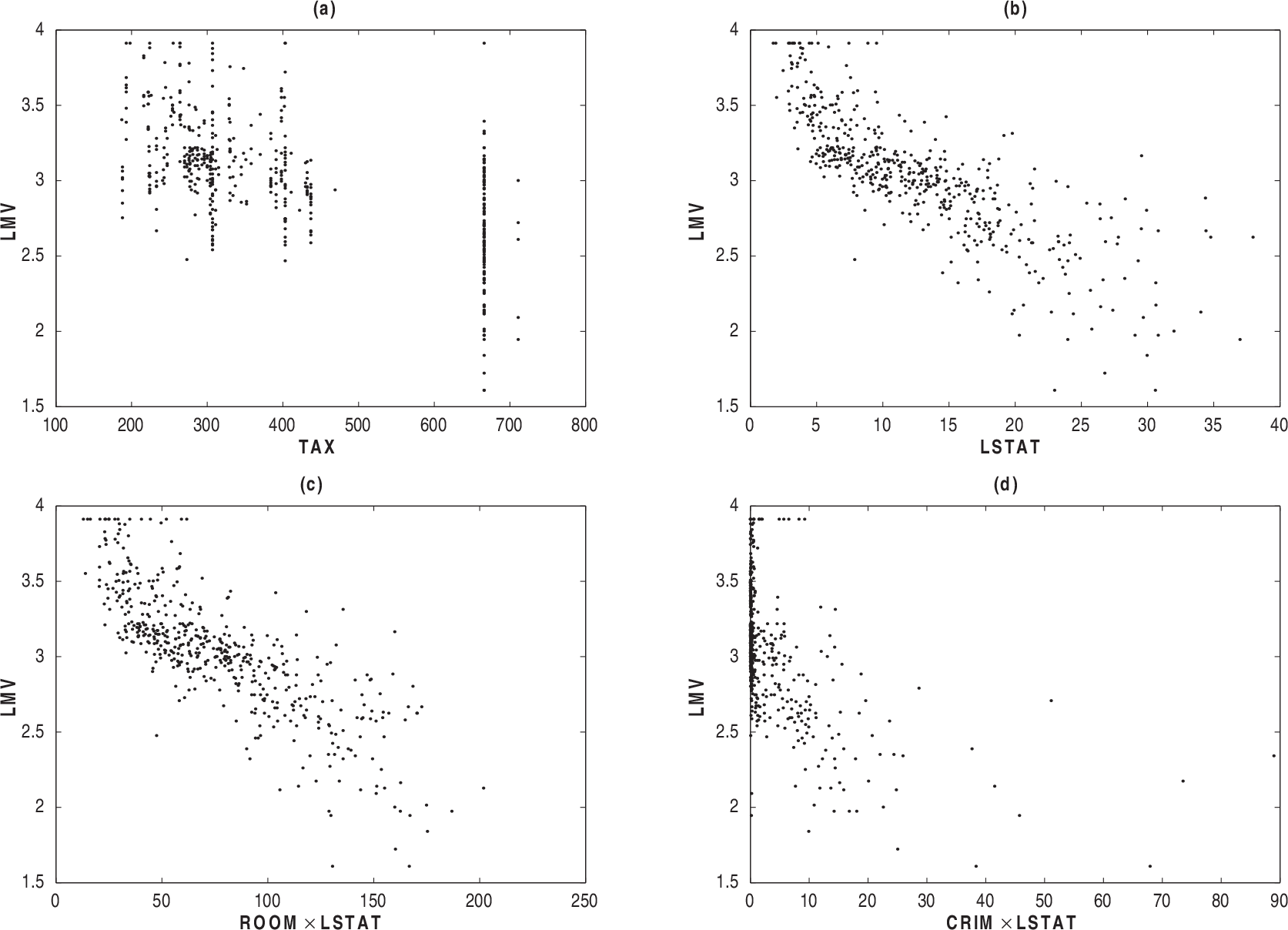
In our application we will consider the house prices dataset that has been reported by Harrison and Rubinfeld (1978). The aim of the study is to assess the association of house prices with the air quality of the neighbourhood by using regression models. The outcome variable LMV (logarithm of the median house price in US$ 1 000) is related with 14 explanatory variables; 6 of them are defined from census track and the remaining variables are defined for clusters. Altogether, there are 506 observations. We will work, for the purpose of motivating the PVCMs, with four explanatory variables, LSTAT (% lower status of the population), ROOM (average number of rooms per dwelling), CRIM (per capita crime rate by town) and TAX (full-value property-tax rate per US$ 10 000).

Figure 1:

Scatter plots: LMV versus TAX (a), LMV versus LSTAT, (b) LMV versus ROOM × LSTAT (c) and CRIM × LSTAT (d)

We see in Figure 1(a) that the relationship between LMV and the explanatory variable TAX is linear, whereas the relationship between LMV and LSTAT appear in nonlinear ways (Figure 1(b)). On other hand, Figures 1(c) and 1(d) suggest that the explanatory variables ROOM and CRIM might be interacting with the variable LSTAT in nonlinear fashion. These tendencies suggest a PVCM among LMV and the explanatory variables. First, we adjust a Student-t and normal PVCM. In order to identify outlying observations, the index plots of the Mahalanobis distance is performed in Figures 2(a) and 2(b).

Figure 2:

Index plots of the Mahalanobis distance under normal (a) and Student-t (b) models and between the estimated weights and Mahalanobis distance under Student-t model (c)

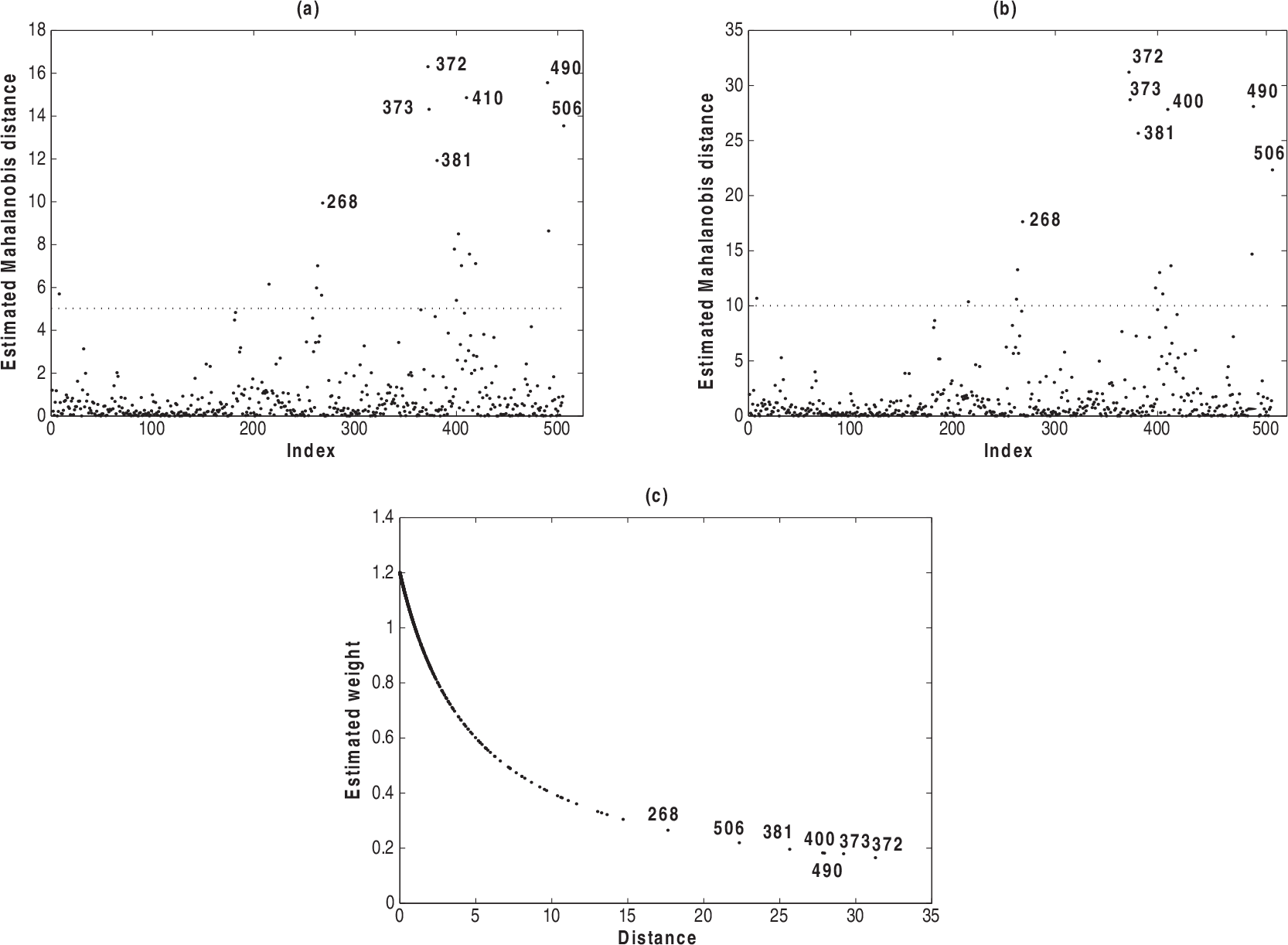
In Figures 2(a), 2(b) and 2(c), we see seven observations albeit with discrepant values. These observations correspond to case 268, 372, 373, 381, 410, 490 and 506. Figure 2(c) displays the estimated weights under the Student-t model and we notice that the estimated weights for the observations described above take the smaller values. In Section 6, we reanalyse this example under heavy-tailed errors for which the maximum penalized likelihood estimates (MPLEs) appear to be less sensitive to the outliers and to some perturbations in the model or data than the estimate from the normal PVCM.

3 The elliptical PVCM

The PVCMs emerge as a powerful tool in statistical modelling because of their flexibility to model explanatory variables effects that can contribute in a parametric way and explanatory variables effects in which the coefficients are allowed to vary as smooth functions of other variables (e.g., time variable). These models are often used in research related to longitudinal, clustered, spatial and hierarchical sampling schemes. In this class of models, usually it is assumed that random errors follow a normal distribution. However, it is well known that in many cases the normal distribution is not appropriate and that the least-squares estimates are sensitive to outlying observations. A possible alternative for dealing with this deficiency is to assume, for example, heavy-tailed distributions for the errors. A class of distributions containing distributions with such features is the class of elliptical distributions. The elliptical class includes all elliptical contoured distributions such as normal, Student-t, power exponential and contaminated normal, among others. The variety of error distributions with different kurtosis coefficients gives more flexibility for analysing datasets from light- and heavy-tailed distributions.

3.1 The model

The PVCM assumes that the relationship between the response variable and the explanatory variables can be represented as

y_{ij} = z_{ij}^{T} α + \sum_{k = 1}^{s} x_{ij}^{(k)} β_{k} (t_{k_{ij}}) + ε_{ij} (i = 1, \dots, n; j = 1, \dots, m_{i}),

(3.1)

where

y_{ij}

denotes the jth measure associated with the ith cluster,

z_{ij}

is (

p \times 1

) vector of explanatory variable values, α is a (

p \times 1

) fixed parameter vector,

β_{k} (\cdot)

(

k = 1, . . ., s

) are unknown smooth arbitrary functions of explanatory variable

t_{k_{ij}}

, associated with the covariates

x_{ij}^{(k)}

, and ε_ij is an random error. The PVCM is an extension of others models that have been proposed in literature. For example, (a) when the functions β_k are all constants, for

k = 1, \dots, s

, and

α

is 0, the PVCM reduces to the classical linear model (LM) and (b) when

α

is 0, the PVCM reduces to the varying-coefficient model (VCM) proposed, for example, by Hastie and Tibshirani (1993).

In order to write model (3.1) in a matrix form, we obtain

y_{i} = Z_{i} α + \sum_{k = 1}^{s} {\tilde{N}}_{k i} β_{k} + \in_{i} (i = 1, \dots, n; i = 1, \dots, m_{i}),

(3.2)

where y_i is a (

m_{i} \times 1

) random vector of observed responses from the ith cluster, Z_i is a (m_i × p) design matrix with rows

z_{i j}^{T}, {\tilde{N}}_{k i} = X_{i}^{(k)} N_{k i}, X_{i}^{(k)} = {diag}_{1 \leq j \leq m_{i}} (x_{i j}^{k}), N_{k i}

is an (

m_{i} \times r_{k}

) incidence matrix with the

(j, l)

th element equal to the indicator

I (t_{k_{ij}} = t_{k_{l}}^{0})

, where

t_{k_{l}}^{0} (l = 1, \dots, r_{k})

denotes the distinct and ordered values of the explanatory variable

t_{k_{i j}}, β_{k} = {(ψ_{k_{1}}, \dots, ψ_{k_{r_{k}}})}^{T}

is a

(r_{k} \times 1)

vector of parameters with

ψ_{k_{l}} = β_{k} (t_{k_{l}}^{0}), f o r l = 1, \dots, r_{k}, a n d \in \in_{i} = (\in_{i} 1, \dots \in_{i m_{i}}) T is an (m_{i} \times 1)

vector of within-cluster errors. Additionally, denoting

y = {(y_{1}^{T}, \dots y_{n}^{T})}^{T}, Z, {\tilde{N}}_{k}

and ∈ similarly, we can also write model (3.2) as

y = Z α + {\tilde{N}}_{1} β_{1} + \dots + {\tilde{N}}_{s} β_{s} + \in .

3.2 Distribution assumption

We will assume that εi follows an elliptical distribution with location parameter 0 and scale matrix Σi (see, e.g., Fang et al., 1990). Consequently, the distribution of yi is given by

y_{i} ~ {El}_{m i} (Z_{i} α + \sum_{k = 1}^{s} {\tilde{N}}_{k i} β_{k}, \sum_{i}) (i = 1, \dots, n) .

In order to ensure that the random vector y_i admits a density for all $y_{i} \in R^{m_{i}}$ with respect to the Lebesgue measure, we will assume the matrix $Σ_{i}$ positive-definite with structure given by $Σ_{i} = Σ_{i} (τ)$ , where $τ = (τ_{1}, \dots, τ_{d})^{T}$ . Then, the density function of the random vector of observed responses $y_{i}$ is given by

f (y_{i}) = {|Σ_{i}|}^{- 1 / 2} g (δ_{i}) (i = 1, \dots, n),

where

δ_{i} = r_{i}^{T} Σ_{i}^{- 1} r_{i}

is the Mahalanobis distance,

r_{i} = y_{i} - μ_{i}

, with

μ_{i} = Z_{i} α + \sum_{k = 1}^{s} {\tilde{N}}_{ki} β_{k}

, and

g (\cdot)

is a function of

R \to [0, \infty]

known as the density generator function. Note that, when exists, the mean E

(y_{i}) = μ_{i}

and covariance–variance matrix

cov (y_{i}) = ξ i Σ i

. In particular, for the Student-t, we have

ξ_{i} = \frac{ν_{i}}{ν_{i} - 2}

(ν_{i} > 2)

, where ν_i denotes the df.

3.3 Penalized function

Let $θ = (α^{T}, β_{1}^{T}, \dots, β_{s}^{T}, τ^{T})^{T} \in Θ \subseteq R^{p^{*}}$ , where $p^{*} = p + r + d$ , with $r = \sum_{k = 1}^{s} r_{k}$ . The log-likelihood function associated to $θ$ is given by

L (θ) = \sum_{i = 1}^{n} L_{i} (θ),

where

L_{i} (θ) = - \frac{1}{2} log | Σ_{i} | + log g (δ_{i})

. It is a known fact that maximizing the log-likelihood function without imposing restrictions over the nonparametric functions may cause overfitting and non-identification of α (see, for instance, Green, 1987). A well-known procedure that can solve this problem is based on the idea of log-likelihood penalization and consists in incorporating a penalty function over each function

β_{k}

such that

L_{p} (θ, λ_{1}, \dots, λ_{s}) = L (θ) + \sum_{k = 1}^{s} λ_{k}^{*} J (β_{k}),

where

J (β_{k})

denotes the penalty function over

β_{k}

and

λ_{k}^{*} = λ^{*} (λ_{k})

is a constant that depends on the parameter

λ_{k} \geq 0

. In this article, we will consider penalty functions of type

J (β_{k}) = {\int_{a_{k}}^{b_{k}} [β_{k}^{(l)} (t_{k})]}^{2} {dt}_{k},

where

β_{k}^{(l)} (t_{k}) = \frac{d^{l}}{d t^{l}} β (t_{k})

t_{k_{l}}^{0} \in [a_{k}, b_{k}]

, and the functions

β_{k}

’s belong to the Sobolev function space

W_{2}^{(ı)} = {β_{k} : β_{k}, β_{k}^{(1)}, \dots, β_{k}^{(ı - 1)} abs . cont ., β_{k}^{(ı)} \in L^{2} [a_{k}, b_{k}]} .

When $ı = 2$ , the estimation of $β_{k}$ leads to a smooth cubic spline with knots at the points $t_{k_{l}}^{0}$ , for $l = 1, \dots, r_{k}$ . According to Green and Silverman (1994), we may express the penalty function as

J (β_{k}) = β_{k}^{T} K_{k} β_{k},

where

K_{k}

is a (

r_{k} \times r_{k}

) nonnegative definite smoothing matrix associated with the

k

th explanatory variable that depends only on the knots. Then, if we consider

λ_{k}^{*} = - λ_{k} / 2

, the penalized log-likelihood function can be expressed as

L_{p} (θ, λ) = L (θ) - \sum_{k = 1}^{s} \frac{λ_{k}}{2} β_{k}^{T} K_{k} β_{k},

(3.3)

where

λ = (λ_{1}, \dots, λ_{s})^{T}

denotes a (

s \times 1

) vector of smoothing parameters that controls the trade-off between goodness of fit and the smoothness-estimated functions. A discussion of the selection of smoothing parameters is presented below.

4 Estimation and inference on the parameters

In this section, we discuss some aspects of estimation and inference in elliptical PVCMs. In the first subsection, we discuss the estimation of α, β’s and τ based on penalized log-likelihood function. Then, we describe a procedure for calculating the approximate standard errors of the parameter estimates and we derive one approximate standard error bands (SEBs) for the coefficients functions. In the following subsections, we present a discussion on df estimation and smoothing parameters selection.

4.1 Maximizing the penalized log-likelihood function

Because $β_{k}$ ’s are infinite-dimensional parameters, we consider the MPLE of θ, which leads to a natural cubic spline estimate of $β_{k}$ ’s. Specifically, the value of θ that maximizes $L_{p} (θ, λ)$ over Θ, denoted by $\hat{θ}$ , is named MPLE and satisfies

L_{p} (\hat{θ}, λ) \geq \sup_{θ \in Θ} L_{p} (θ, λ) .

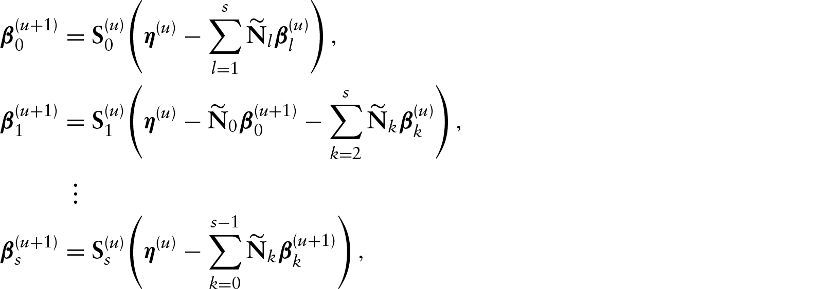
The determination of the MPLE $\hat{θ}$ can be performed by considering successive maximizations as described, for instance, in Gourieroux and Monfort (1995, Chapter 7). Specifically, for $λ$ fixed and $s = 2$ , for example, the solution $\hat{θ}$ to the maximization problem

_{θ \in Θ}^{\max} L_{p} (θ, λ) =_{α, β_{1}, β_{2}, τ}^{\max} L_{p} (α, β_{1}, β_{2}, τ, λ)

can be obtained via the following four-step procedure (see also Ibacache-Pulgar et al., 2012):

First, we maximize the function $L_{p} (α, β_{1}, β_{2}, τ, λ)$ over $α$ by keeping fixed the parameters $β_{1}, β_{2}$ and τ. The maximum value, $\hat{α} = \hat{α} (β_{1}, β_{2}, τ)$ , is attained for values of $α$ in a set $B (β_{1}, β_{2}, τ)$ depending on the parameters $β_{1}, β_{2}$ and $τ$ . Thus, if $α$ $\in$ $B (β_{1}, β_{2}, τ)$ , then the penalized log-likelihood value is

L_{p}^{c} (β_{1}, β_{2}, τ, λ) = max_{α} L_{p} (α, β_{1}, β_{2}, τ, λ) .

Here, $L_{p}^{c}$ is called the concentred penalized log-likelihood in $α$ .

Then, we maximize $L_{p}^{c} (β_{1}, β_{2}, τ, λ) = L_{p} (\hat{α}, β_{1}, β_{2}, τ, λ)$ over $β_{1}$ by keeping $β_{2}$ and $τ$ fixed. The maximum value, ${\hat{β}}_{1} = {\hat{β}}_{1} (β_{2}, τ)$ , is attained for values of $β_{1}$ in a set $F_{1} (β_{2}, τ)$ depending on the parameter $β_{2}$ and $τ$ . Therefore, if $β_{1}$ $\in$ $F_{1} (β_{2}, τ)$ , then the penalized log-likelihood value is

L_{p}^{c} (β_{2}, τ, λ) = \max_{β_{1}} L_{p}^{c} (β_{1}, β_{2}, τ, λ) .

Here,

L_{p}^{c}

is called the concentred penalized log-likelihood in

α

and

β_{1}

Now, we maximize $L_{p}^{c} (β_{2}, τ, λ) = L_{p} (\hat{α}, {\hat{β}}_{1}, β_{2}, τ, λ)$ over $β_{2}$ by keeping $τ$ fixed. The maximum value, ${\hat{β}}_{2} = {\hat{β}}_{2} (τ)$ , is attained for values of $β_{2}$ in a set $F_{2} (τ)$ depending on the parameter $τ$ . Therefore, if $β_{2}$ $\in$ $F_{2} (τ)$ , then the penalized log-likelihood value is

L_{p}^{c} (τ, λ) = \max_{β_{2}} L_{p}^{c} (β_{2}, τ, λ) .

Here,

L_{p}^{c}

is called the concentred penalized log-likelihood in

α

β_{1}

and

β_{2}

Finally, we maximize $L_{p}^{c} (τ, λ) = L_{p} (\hat{α}, {\hat{β}}_{1}, {\hat{β}}_{2}, τ, λ)$ over $τ$ . The maximum value, $\hat{τ}$ , is attained on a set $C$ of $τ$ values.

The four-step procedure can be generalized for $3 \leq k \leq s$ .

4.2 Fisher score and weighted back-fitting algorithms

Let $β_{0} = α$ and ${\tilde{N}}_{0} = Z$ , $W_{v} = {blockdiag}_{1 \leq i \leq n} (v_{i} W_{i})$ , $W^{*} = {blockdiag}_{1 \leq i \leq n} (\frac{4 d_{g_{i}}}{m_{i}} W_{i})$ , with $W_{i} = Σ_{i}^{- 1}$ and $d_{g_{i}} = E (ζ_{g}^{2} (δ_{i}) δ_{i})$ , $v_{i} = - 2 ζ_{g} (δ_{i})$ and $ζ_{g} (δ_{i}) = \frac{d log g (δ_{i})}{d δ_{i}}$ . For simplicity, consider $α$ , $W_{v}$ and $W^{*}$ fixed. The four-step procedure (1–4) described in Subsection 4.1 can be solved, for $1 \leq k \leq s$ , by using the following Fisher scoring algorithm (see, for instance, Rigby and Stasinopoulus, 2005):

\begin{matrix} (\begin{matrix} I & S_{0}^{(u)} {\tilde{N}}_{1} & \dots & S_{0}^{(u)} {\tilde{N}}_{s} \\ S_{1}^{(u)} Z & I & \dots & S_{1}^{(u)} {\tilde{N}}_{s} \\ ⋮ & ⋮ & ⋱ & ⋮ \\ S_{s}^{(u)} Z & S_{s}^{(u)} {\tilde{N}}_{1} & \dots & I \end{matrix}) (\begin{matrix} β_{0}^{(u + 1)} \\ β_{1}^{(u + 1)} \\ ⋮ \\ β_{s}^{(u + 1)} \end{matrix}) = (\begin{matrix} S_{0}^{(u)} η^{(u)} \\ S_{1}^{(u)} η^{(u)} \\ ⋮ \\ S_{s}^{(u)} η^{(u)} \end{matrix}), \end{matrix}

(4.1)

where

η^{(u)} = μ + W^{*^{- 1}} W_{v} (y - μ)

|_{θ^{(u)}}

and

S_{k}^{(u)} = S_{k}

|_{θ^{(u)}}

, with

y = (y_{1}^{T}, \dots, y_{n}^{T})^{T}

μ = (μ_{1}^{T}, \dots, μ_{n}^{T})^{T}

and

\begin{matrix} S_{k}^{(u)} & = & \{\begin{matrix} ({\tilde{N}}_{0}^{T} W^{*} {\tilde{N}}_{0})^{- 1} {\tilde{N}}_{0}^{T} W^{*} |_{θ^{(u)}} & k = 0 \\ ({\tilde{N}}_{k}^{T} W^{*} {\tilde{N}}_{k} + λ_{k} K_{k})^{- 1} {\tilde{N}}_{k}^{T} W^{*} & (k = 1, \dots, s) . \end{matrix} \end{matrix}

Then, the back-fitting (Gauss–Seidel) iterations that are used to solve the equations system (4.1) take the form

β_{k}^{(u + 1)} = S_{k}^{(u)} (η^{(u)} - \sum_{l = 0, l \neq k}^{s} {\tilde{N}}_{l} β_{l}^{(u)}) .

(4.2)

Note that the back-fitting algorithm (4.2) depends on the elliptical distribution through the weight matrices

W^{*}

. In particular, under normal distribution for which

v_{i} = 1

and

d_{g_{i}} = \frac{m_{i}}{4}

, we have that

W_{v} = W^{*} = {blockdiag}_{1 \leq i \leq n} (W_{i})

and, therefore,

η = y

. In addition, the system of equation (4.1) is consistent and the back-fitting algorithm (4.2) converges to a solution for any starting value if the weight matrix involved is symmetric and defined positive (see, for instance, Berhane and Tibshirani, 1998). Further, we have that this solution is unique when there is no concurvity in the data.

4.3 Joint iterative process

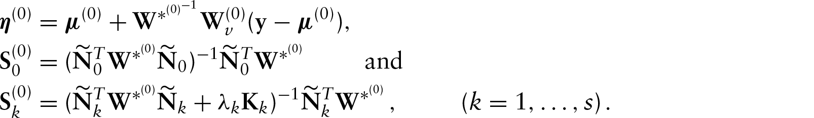
The solution of the estimating equation system (4.1) to obtain the MPLE of $θ$ may be attained by iterating between a weighted back-fitting algorithm with weight matrix $W^{*}$ and a Fisher score algorithm to obtain maximum likelihood estimation of the parameter $τ$ , which is equivalent to the following iterative process:

Initialize:

a. Fitting a PVCM under normal errors to get $β_{J}^{(0)}$ ( $J = 0, 1, \dots, s$ ).

b. Getting starting value for $τ$ by using the fitted values from a.

c. From the current value $θ^{(0)} = (β_{0}^{(0)^{T}}, β_{1}^{(0)^{T}}, \dots, β_{s}^{(0)^{T}}, τ^{(0)})^{T}$ obtaining the weight matrix $Σ_{i}^{(0)} = Σ_{i}$ $|_{θ^{(0)}}$ , $W^{*^{(0)}}$ , $v_{i}^{(0)} = v_{i}$ $|_{θ (0)}$ , $W_{i}^{(0)} = Σ_{i}^{(0) - 1}$ and $W_{v}^{(0)} = {blockdiag}_{1 \leq i \leq n} (v_{i}^{(0)} W_{i}^{(0)})$ . Then, obtaining

\begin{matrix} η^{(0)} & = & μ^{(0)} + W^{*^{(0)^{- 1}}} W_{v}^{(0)} (y - μ^{(0)}), \\ S_{0}^{(0)} & = & ({\tilde{N}}_{0}^{T} W^{*^{(0)}} {\tilde{N}}_{0})^{- 1} {\tilde{N}}_{0}^{T} W^{*^{(0)}} and \\ S_{k}^{(0)} & = & ({\tilde{N}}_{k}^{T} W^{*^{(0)}} {\tilde{N}}_{k} + λ_{k} K_{k})^{- 1} {\tilde{N}}_{k}^{T} W^{*^{(0)}}, (k = 1, \dots, s) . \end{matrix}

Step 1: Iterating repeatedly by cycling between the following equations:

\begin{matrix} β_{0}^{(u + 1)} & = & S_{0}^{(u)} (η^{(u)} - \sum_{l = 1}^{s} {\tilde{N}}_{l} β_{l}^{(u)}), \\ β_{1}^{(u + 1)} & = & S_{1}^{(u)} (η^{(u)} - {\tilde{N}}_{0} β_{0}^{(u + 1)} \sum_{k = 2}^{s} {\tilde{N}}_{k} β_{k}^{(u)}), \\ ⋮ \\ β_{s}^{(u + 1)} & = & S_{s}^{(u)} (η^{(u)} - \sum_{k = 0}^{s - 1} {\tilde{N}}_{k} β_{k}^{(u + 1)}), \end{matrix}

for

u = 0, 1, \dots

. Repeating 2 replacing

β_{J}^{(u)}

β_{J}^{(u + 1)}

(

J = 0, 1, \dots, s

) until convergence criterion

Δ_{u} (β_{J}^{(u + 1)}, β_{J}^{(u)}) = \sum_{J = 0}^{s} ∥ β_{J}^{(u + 1)} - β_{J}^{(u)} ∥ / \sum_{J = 0}^{s} ∥ β_{J}^{(u)} ∥

is below some small threshold (Hastie and Tibshirani, 1990).

Step 2: For current values $β_{J}^{(u + 1)}$ ( $J = 0, 1, \dots, s$ ), obtaining $τ^{(u + 1)}$ by using

τ^{(u + 1)} = τ^{(u)} - E {\frac{\partial^{2} L_{p}^{c} (τ, λ)}{\partial τ \partial τ^{T}}}^{- 1} \frac{\partial L_{p}^{c} (τ, λ)}{\partial τ} | θ^{(u)} .

Iterating between 2 and 3 by replacing $β_{J}^{(0)}$ ( $J = 0, 1, \dots, s$ ) and $τ^{(0)}$ by $β_{J}^{(u + 1)}$ and $τ^{(u + 1)}$ respectively until convergence.

Note that under Student-t distribution (df $= ν_{i}$ ) the current weight $v_{i}^{(u)} = \frac{ν_{i} + m_{i}}{ν_{i} + δ_{i}^{(u)}}$ , with $δ_{i}^{(u)}$ $=$ $δ_{i}$ $|_{θ^{(u)}}$ , is inversely proportional to the distance between the observed value $y_{i}$ and its current predicted value $μ_{i}^{(u)}$ , so that outlying observations tend to have small weights in the estimation process.

4.4 Approximate standard errors

In this work, we derive the covariance matrix of $\hat{θ}$ from the inverse of the expected information matrix $ℐ_{p}$ , defined in Appendix. Therefore, the approximate covariance matrix of $\hat{θ}$ is given as

\hat{Cov} (\hat{θ}) \approx ℐ_{p}^{- 1} | \hat{θ}

By using elemental properties to partitioned matrix, we can show that the inverse matrix of

ℐ_{p}

assumes the following block-diagonal form:

\begin{matrix} ℐ_{p}^{- 1} & = & (\begin{matrix} {(ℐ_{α α} - ℐ_{α β} ℐ_{β β}^{- 1} ℐ_{β α}^{T})}^{- 1} & ℐ_{α α} ℐ_{α β} ℐ_{β β}^{- 1} & 0 \\ {(ℐ_{α α} ℐ_{α β} ℐ_{β β}^{- 1})}^{T} & {(ℐ_{β β} - ℐ_{α β}^{T} ℐ_{α α}^{- 1} ℐ_{α β})}^{- 1} & 0 \\ 0 & 0 & ℐ_{τ τ}^{- 1} \end{matrix}), \end{matrix}

where

\begin{matrix} ℐ_{α α} & = & Z^{T} W^{*} Z, \\ ℐ_{α β} & = & (\begin{matrix} Z^{T} W^{*} {\tilde{N}}_{1} & \dots & Z^{T} W^{*} {\tilde{N}}_{s} \end{matrix}) \end{matrix}

and

\begin{matrix} ℐ_{β β} & = & (\begin{matrix} {\tilde{N}}_{1}^{T} W^{*} {\tilde{N}}_{1} + λ_{1} K_{1} & \dots & {\tilde{N}}_{1}^{T} W^{*} {\tilde{N}}_{s} \\ ⋮ & ⋰ & ⋮ \\ {\tilde{N}}_{s}^{T} W^{*} {\tilde{N}}_{1} & \dots & {\tilde{N}}_{s}^{T} W^{*} {\tilde{N}}_{s} + λ_{s} K_{s} \end{matrix}) . \end{matrix}

In particular, if we are interested in drawing inferences for

α

and

(β_{1}, \dots, β_{s})

, the approximate covariance matrices can be estimated by using the corresponding block-diagonal matrices obtained from

ℐ_{p}^{- 1}

, that is,

\begin{matrix} \hat{Cov} (\hat{α}) & \approx & {(ℐ_{α α} - ℐ_{α β} ℐ_{β β}^{- 1} ℐ_{α β}^{T})}^{- 1} |_{\hat{θ}} \end{matrix}

and

\begin{matrix} \hat{Cov} ({\hat{β}}_{1}, \dots, {\hat{β}}_{s}) & \approx & {(ℐ_{β β} - ℐ_{α β}^{T} ℐ_{α α}^{- 1} ℐ_{α β})}^{- 1} |_{\hat{θ}} . \end{matrix}

(4.3)

4.5 Approximate SEBs

By using variance–covariance matrix (4.3), we can construct an approximate pointwise SEB for $β_{k} (\cdot)$ that allows us to assess how accurate the estimator $\hat{β_{k}} (\cdot)$ is at different locations within the range of interest. For example, we can consider the following approximate pointwise SEB (Hastie and Tibshirani, 1990):

\begin{matrix} {SEB}_{approx} (β_{k} (t_{l}^{0})) & = & {\hat{β}}_{k} (t_{l}^{0}) \pm 2 \sqrt{\hat{Var} ({\hat{β}}_{k} (t_{l}^{0}))} (l = 1, \dots, r), \end{matrix}

where

Var ({\hat{β}}_{k} (t_{l}))

is the

l

th principal diagonal element of the matrix (4.3).

4.6 On degrees of freedom

In the elliptical PVCM, the df associated with the $k$ th coefficient function is given by (see, for instance, Hastie and Tibshirani, 1990)

df (λ_{k}) = tr ({\tilde{N}}_{k} S_{k}) = tr ({\tilde{S}}_{k}),

(4.4)

which measure the individual effect contribution of the

k

th component, with

S_{k}

defined in Section 4.2. Following Eilers and Marx (1996), we can write

tr {{\tilde{S}}_{k}}

tr {{\tilde{S}}_{k}} = \sum_{j = 1}^{r_{k}} \frac{1}{1 + λ_{k} ℓ_{j}} \approx 2 + \sum_{j = 3}^{r_{k}} \frac{1}{1 + λ_{k} ℓ_{j}},

(4.5)

where

ℓ_{j}

, for

j = 1, \dots, r_{k}

, are the eigenvalues of the matrix

Q_{{\tilde{N}}_{k}}^{- 1 / 2} Q_{λ_{k}} Q_{{\tilde{N}}_{k}}^{- 1 / 2}

, for

k = 1, \dots, s

, with

Q_{{\tilde{N}}_{k}} = {\tilde{N}}_{k}^{T} W^{*} {\tilde{N}}_{k}

and

Q_{λ_{k}} = λ_{k} K_{k}

. It is important to note that (a)

df (λ_{k}) = tr {{\tilde{S}}_{k}}

is a monotonically decreasing function of

λ_{k}

; (b)

df (λ_{k}) \to 2 + r_{k}

λ_{k} \to 0

; (c)

df (λ_{k}) \to 2

λ_{k} \to \infty

; and (d)

2 \leq df (λ_{k}) \leq 2 + r_{k}

4.7 Choosing the smoothing parameters

In the previous subsections, the smoothing parameters $λ_{k}$ ’s were assumed fixed. However, in practical situations, the smoothing parameters should be selected from the data. When a smoothing spline is used, for example, it is usual to consider the cross-validation method or the generalized cross-validation method (Craven and Wahba, 1979). Alternatively, these parameters may be selected by applying the Akaike information criterion (AIC) (Akaike, 1973); see also Hurvich et al. (1998) and Simonoff and Tsai (1999) in the semiparametric context. In this work, we will apply the following procedure based on the AIC (see, for instance, Ibacache-Pulgar et al., 2013):

For simplicity, consider $s = 2$ .

a. Select $m$ values $u_{k_{ℓ}} \in (0, 1)$ and obtain the smoothing parameter values $λ_{k_{ℓ}} = u_{k_{ℓ}} / (1 - u_{k_{ℓ}})$ , for $ℓ = 1, \dots, m$ .

b. From Equation (4.4), obtain ${df}_{k_{ℓ}} = df (λ_{k_{ℓ}})$ and perform a dispersion graph between $λ_{k_{ℓ}}$ and ${df}_{k_{ℓ}}$ . From Equation (4.5), a reciprocal relationship is expected between $λ_{k}$ and $df (λ_{k_{ℓ}})$ .

Select a range for the smoothing parameters.

a. Obtain an appropriate regression obtaining the fitted equation ${\hat{λ}}_{k_{ℓ}} = η ({df}_{k_{ℓ}})$ , where $η (\cdot)$ denotes the regression function.

b. Since the relationship between $λ_{k}$ and ${df}_{k}$ is monotonically decreasing, we may obtain from the fitted regression a range $[λ_{k}^{L_{k}}, λ_{k}^{U_{k}}]$ for $λ_{k}$ given a range for the df. For example, if we consider the range [2,16], we have that $λ_{k}^{U_{k}} = η (16)$ and $λ_{k}^{L_{k}} = η (2)$ .

Minimize the $AIC$ .

The suggestion is to select a grid of values from the range $[λ_{k}^{L_{k}}, λ_{k}^{U_{k}}]$ and choose the smoothing parameters values $λ_{k}$ that minimizes

AIC (λ) = - 2 L_{p} (θ, λ) |_{\hat{θ}} + 2 [1 + p + df (λ)],

where

λ = (λ_{1}, λ_{2})^{T}

p

denotes the number of parameters in

α

, and

df (λ) = \sum_{k = 1}^{2} df (λ_{k})

denotes approximately the number of effective parameters involved in modelling of the nonparametric effects.

5 Local influence measure

In this section, we present the local influence method and derive the perturbation matrix for different perturbation schemes under elliptical PVCM.

5.1 The method

Let $ω = (ω_{1}, \dots, ω_{n})^{T}$ be an ( $n \times 1$ ) vector of perturbations restricted to some open subset $Ω$ $\in$ $R^{n}$ and the logarithm of the perturbed penalized likelihood denoted by $L_{p} (θ, λ | ω)$ . Suppose that there is a point $ω_{0}$ $\in$ $Ω$ that represents no perturbation of the data so that $L_{p} (θ, λ | ω_{0}) = L_{p} (θ, λ)$ . To assess the influence of minor perturbations on $\hat{θ}$ , we consider the likelihood displacement $LD (ω) = 2 [L_{p} (\hat{θ}, λ) - L_{p} ({\hat{θ}}_{ω}, λ)] \geq 0$ , where ${\hat{θ}}_{ω}$ is the MPLE under $L_{p} (θ, λ | ω)$ . The measure $LD (ω)$ is useful for assessing the distance between $\hat{θ}$ and ${\hat{θ}}_{ω}$ . Cook (1986) suggested studying the local behavior of $LD (ω)$ around $ω_{0}$ . The procedure consists in selecting a unit direction $ℓ$ $\in$ $Ω$ ( $∥ ℓ ∥ = 1$ ), and then to consider the plot of $LD (ω_{0} + a ℓ)$ against $a$ , where $a$ $\in$ $R$ . This plot is called lifted line. Each lifted line can be characterized by considering the normal curvature $C_{ℓ} (θ)$ around $a = 0$ . The suggestion is to consider the direction $ℓ = ℓ_{\max}$ corresponding to the largest curvature $C_{ℓ_{\max}} (θ)$ . The index plot of $ℓ_{\max}$ may reveal those observations that under small perturbations exercise notable influence on $LD (ω)$ . According to Cook (1986), the normal curvature in the unitary direction $ℓ$ is given by $C_{ℓ} (θ) = - 2 {ℓ^{T} Δ_{p}^{T} L_{p}^{- 1} Δ_{p} ℓ}$ , where $L_{p}$ is the Hessian matrix defined in Appendix and $Δ_{p}$ is the perturbation matrix.

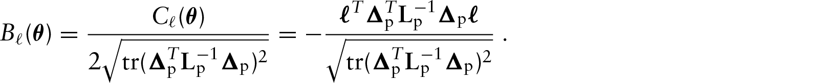
5.2 Conformal normal curvature

In order to have a curvature invariant under uniform change of scale, Poon and Poon (1999) proposed the conformal normal curvature defined as

B_{ℓ} (θ) = \frac{C_{ℓ} (θ)}{2 \sqrt{tr (Δ_{p}^{T} L_{p}^{- 1} Δ_{p})^{2}}} = - \frac{ℓ^{T} Δ_{p}^{T} L_{p}^{- 1} Δ_{p} ℓ}{\sqrt{tr (Δ_{p}^{T} L_{p}^{- 1} Δ_{p})^{2}}} .

This curvature is characterized to allow for any unitary direction

ℓ

that

0 \leq B_{ℓ} (θ) \leq 1

. A suggestion is to consider the direction

ℓ = ℓ_{\max}

corresponding to the largest curvature

B_{ℓ_{\max}} (θ)

or, alternatively, evaluating the normal curvature at the direction

ℓ = e_{i}

, where

e_{i}

is an (

n \times 1

) vector with 1 in the

i

th position and 0s in the remaining positions, and observing the index plot of

B_{e_{i}} (θ)

5.3 Normal curvature derivation

In this subsection, we present the expressions of the elements of the ( $p^{*} \times n$ ) $Δ_{p}$ matrix for case-weight, scale matrix and explanatory variable perturbation schemes.

5.3.1 Case-weight perturbation

Let us consider the attributed weights for the observations in the penalized log-likelihood function as

L_{p} (θ, λ | ω) = \sum_{i = 1}^{n} ω_{i} L_{i} (θ) - \sum_{k = 1}^{s} \frac{λ_{k}}{2} β_{k}^{T} K_{k} β_{k} (i = 1, \dots, n),

(5.1)

where

ω = (ω_{1}, \dots, ω_{n})^{T}

is the vector of weights, with

0 \leq ω_{i} \leq 1

. In this case,

ω_{0} = (1, \dots, 1)^{T}

. Differentiating (5.1) with respect to the elements of

θ

and

ω_{i}

, we obtain the expressions

\begin{matrix} \frac{\partial^{2} L_{p_{i}} (θ, λ | ω)}{\partial α \partial ω_{i}} |_{\hat{θ}, ω_{0}} & = & v_{i} Z_{i}^{T} Σ_{i}^{- 1} r_{i} |_{\hat{θ}, ω_{0}}, \\ \frac{\partial^{2} L_{p_{i}} (θ, λ | ω)}{\partial β_{k} \partial ω_{i}} |_{\hat{θ}, ω_{0}} & = & v_{i} {\tilde{N}}_{ki}^{T} Σ_{i}^{- 1} r_{i} |_{\hat{θ}, ω_{0}} (k = 1, \dots, s) \end{matrix}

and

\begin{matrix} \frac{\partial^{2} L_{p_{i}} (θ, λ | ω)}{\partial τ_{J} \partial ω_{i}} |_{\hat{θ}, ω_{0}} & = & - \frac{1}{2} tr (Σ_{i}^{- 1} \frac{\partial Σ_{i}}{\partial τ_{J}}) + \frac{1}{2} v_{i} r_{i}^{T} Σ_{i}^{- 1} \frac{\partial Σ_{i}}{\partial τ_{J}} Σ_{i}^{- 1} r_{i} |_{\hat{θ}, ω_{0}}, \end{matrix}

for

i = 1, \dots, n

and

J = 1, \dots, d

5.3.2 Scale perturbation

Under the scale parameter perturbation scheme, we assume that

y_{i} \sim {El}_{m_{i}} (μ_{i}, ω_{i}^{- 1} Σ_{i}) (i = 1, \dots, n),

where

ω = (ω_{1}, \dots, ω_{n})^{T}

is the vector of perturbations, with

ω_{i} > 0

. In this case,

ω_{0} = (1, \dots, 1)^{T}

such that

L_{p} (θ, λ | ω_{0}) = L_{p} (θ, λ)

. Taking differentials of

L_{p} (θ, λ | ω)

with respect to the elements of

θ

and

ω_{i}

, simple algebra yields

\begin{array}{l} {\frac{\partial^{2} L_{p_{i}} (θ, λ | ω)}{\partial α \partial ω_{i}} |}_{\hat{θ}, ω_{0}} = {{v^{'}}_{i} δ_{i} + v_{i}} Z_{i}^{T} Σ_{i}^{- 1} r_{i} |_{\hat{θ}, ω_{0}}, \\ {\frac{\partial^{2} L_{p_{i}} (θ, λ | ω)}{\partial β_{k} \partial ω_{i}} |}_{\hat{θ}, ω_{0}} = {{v^{'}}_{i} δ_{i} + v_{i}} {\tilde{N}}_{k i}^{T} Σ_{i}^{- 1} r_{i} |_{_{\hat{θ}, ω_{0}}} (k = 1, \dots, s) \end{array}

and

\begin{matrix} \frac{\partial^{2} L_{p_{i}} (θ, λ | ω)}{\partial τ_{J} \partial ω_{i}} |_{\hat{θ}, ω_{0}} & = & \frac{1}{2} {v_{i}^{'} δ_{i} + v_{i}} r_{i}^{T} Σ_{i}^{- 1} \frac{\partial Σ_{i}}{\partial τ_{J}} Σ_{i}^{- 1} r_{i} |_{\hat{θ}, ω_{0}}, \end{matrix}

for

i = 1, \dots, n

and

J = 1, \dots, d

5.3.3 Explanatory variable perturbation

Here, the $k$ th explanatory variable (assumed continuous) is perturbed by considering additive perturbation schemes, namely $z_{i k ω} = z_{i k} + ω_{i}$ , where $z_{i k}$ denotes the $k$ th column of the matrix $Z_{i}$ and $ω_{i} = (ω_{1}, \dots, ω_{m_{i}})^{T}$ is the vector of perturbations. In this case, the design matrix $_{i}$ associated to the parametric components of the model is replaced by $Z_{i ω} = (\begin{array}{ccccc} z_{i 1} & \dots & z_{i k ω} & \dots & z_{ip} \end{array})$ . Thus, the perturbed penalized log-likelihood function is constructed from (3.3) with $Z_{i}$ replaced by $Z_{i ω}$ , that is,

L_{p} (θ, λ | ω) = L (θ | ω) - \sum_{k = 1}^{s} \frac{λ_{k}}{2} β_{k}^{T} K_{k} β_{k} (i = 1, \dots, n),

(5.2)

where

L (\cdot)

is given by (3.3) and evaluated at

δ_{i ω} = r_{i ω}^{T} Σ_{i}^{- 1} r_{i ω}

, with

r_{i ω} = y_{i} - μ_{i ω}

and

μ_{i} = Z_{i ω} α + \sum_{k = 1}^{s} {\tilde{N}}_{ki} β_{k}

. In this case, we have

ω_{0} = 0

\in

R^{n^{*}}

, with

n^{*} = \sum_{i = 1}^{n} m_{i}

. Differentiating (5.2) with respect to

θ

and

ω_{i}

, we obtain

\begin{matrix} \frac{\partial^{2} L_{p_{i}} (θ, λ | ω)}{\partial α \partial ω_{i}^{T}} |_{\hat{θ}, ω_{0}} & = & - 2 v_{i}^{'} z_{i}^{T} Σ_{i}^{- 1} r_{i} r_{i}^{T} Σ_{i}^{- 1} α_{t} - v_{i} {z_{i}^{T} α_{t} - c_{t} r_{i}^{T}} Σ_{i}^{- 1} |_{\hat{θ}, ω_{0}}, \\ \frac{\partial^{2} L_{p_{i}} (θ, λ | ω)}{\partial β_{k} \partial ω_{i}^{T}} |_{\hat{θ}, ω_{0}} & = & - {\tilde{N}}_{ki}^{T} Σ_{i}^{- 1} {2 v_{i}^{'} r_{i} r_{i}^{T} + v_{i} Σ_{i}} Σ_{i}^{- 1} α_{t} |_{\hat{θ}, ω_{0}} (k = 1, \dots, s) \end{matrix}

and

\begin{matrix} \frac{\partial^{2} L_{p_{i}} (θ, λ | ω)}{\partial τ_{J} \partial ω_{i}^{T}} |_{\hat{θ}, ω_{0}} & = & - r_{i}^{T} Σ_{i}^{- 1} \frac{\partial Σ_{i}}{\partial τ_{J}} Σ_{i}^{- 1} {v_{i}^{'} r_{i} r_{i}^{T} + v_{i}^{'} Σ_{i}} Σ_{i}^{- 1} α_{k} |_{\hat{θ}, ω_{0}}, \end{matrix}

for

i = 1, \dots, n

and

J = 1, \dots, d

. Here,

α_{t}

denotes the

t

th element of

α

and

c_{t}

is a (

p \times 1

) vector with 1 in the

t

th position and 0 elsewhere.

6 Application

The dataset reported by Harrison and Rubinfeld (1978) has been analysed by various authors using different models; see, for instance, Belsley et al. (1980) and Ibacache-Pulgar et al. (2013). The descriptive analysis of Section 2 suggests that the relationship between LMV and the explanatory variable TAX is linear (see Figure 1(a)), whereas the relationship between LMV and LSTAT appears in non-linear ways (see Figure 1(b)). On other hand, Figures 1(c) and 1(d) suggest that the explanatory variables ROOM and CRIM might be interacting with the variable LSTAT in nonlinear fashion. These tendencies suggest a PVCM among LMV and the explanatory variables. Specifically, we will assume the following model:

\begin{matrix} y_{i} & = & α_{0} + α_{1} z_{i} +_{β 1} (t_{i}) x_{i}^{(1)} + β_{2} (t_{i}) x_{i}^{(2)} + ε_{i} (i = 1, \dots, 506), \end{matrix}

(6.1)

where

y_{i}

denotes the value of LMV in US$ 1 000,

z_{i}

denotes the value of TAX,

x_{i}^{(1)}

denotes the value of CRIM,

x_{i}^{(2)}

denotes the value of ROOM,

t_{i}

denotes the value of LSTAT from the

i

th experimental unit,

α = (α_{1}, α_{2})^{T}

β_{k}

(

k = 1, 2

) are unknown functions and

ε_{i}

are independent random errors that follow a distribution

El (0, ϕ, g)

6.1 Fitting the models

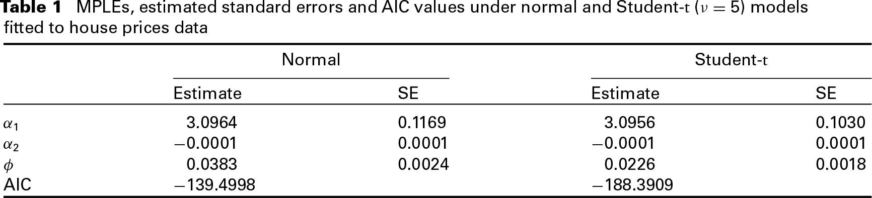
We will compare in the sequel the fits based on normal and Student-t errors. The df $ν = 5$ for the Student-t model was selected by AIC, that is, by defining a grid of values for $ν$ and choosing the one that maximizes the $L_{p} (θ, λ)$ . The MPLE estimates, estimated standard errors and the corresponding AIC for the model (6.1) under normal and Student-t errors are presented in Table 1.

Table 1:

MPLEs, estimated standard errors and AIC values under normal and Student-t ( $ν = 5$ ) models fitted to house prices data

	Normal		Student-t
	Estimate	SE	Estimate	SE
α₁	3.0964	0.1169	3.0956	0.1030
$α_{2}$	$-$ 0.0001	0.0001	$-$ 0.0001	0.0001
$ϕ$	0.0383	0.0024	0.0226	0.0018
AIC	$-$ 139.4998		$-$ 188.3909

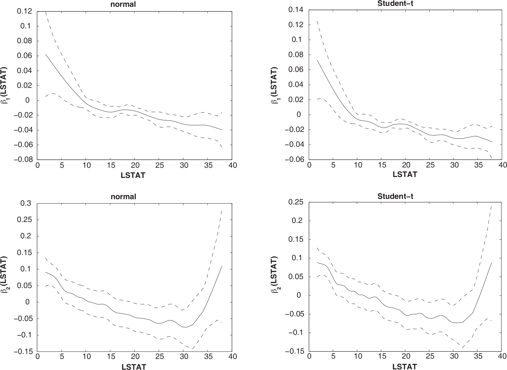
Comparing these results, we may notice a similarity between the estimates $\hat{α}$ under both models, but the standard error for ${\hat{α}}_{1}$ appears to be smaller under the Student-t model. In addition, we may notice that the AIC value under the Student-t model is smaller than the one under the normal model, indicating a superiority of the heavy-tailed model. Figure 3 shows the estimated coefficients functions under both models and their corresponding approximate SEB (dashed curves). The estimated coefficients functions were computed using the smoothing parameters obtained by the method described in Subsection 4.7, specifying the df range as [4,12] for both models. The graphics suggest clearly that the coefficient curves vary with variable LSTAT. Figure 3:

Plots of estimated coefficient functions for the house prices data, and their approximate pointwise SEB denoted by the dashed lines

Figure 4:

Scatter plots of LMV versus fitted LMV: normal (a) and Student-t models (b)

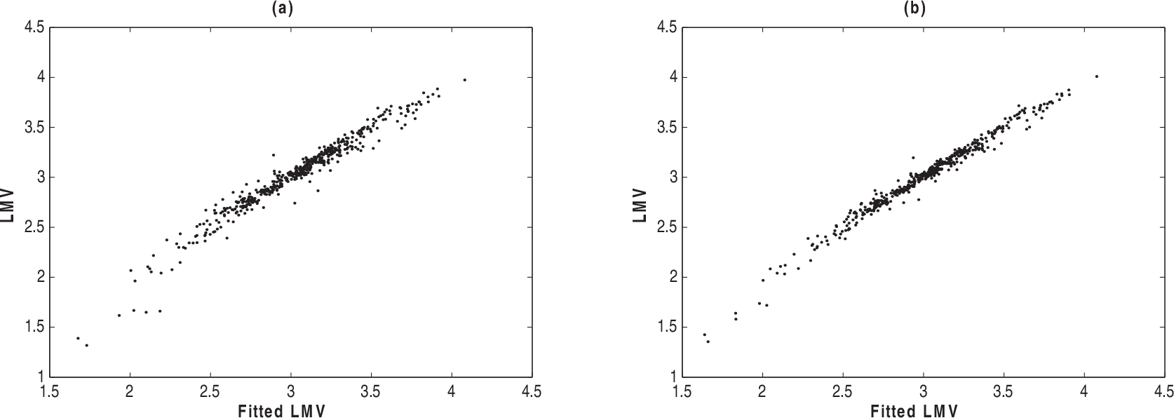
Figure 4 displays the graphics of the LMV versus the fitted LMV from tho models, indicating suitable fits for both models.

It is important to mention that the observations 372, 490, 410, 373, 506, 381 and 268 that appear as possible outliers under Student-t and normal models (see Figures 2(a) and 2(b)), the estimation process under Student-t model assigns them small weights, confirming the robust aspects of the MPLEs against outlying observations under heavier-tailed error models; see Figure 2(c).

6.2 Local influence diagnostics

Now, in order to identify influential observations, we present some index plots of $B_{i} = B_{e_{i}} (ψ)$ , for $ψ = α, β_{1}, β_{2}, ϕ$ . In this application, we will use the approach $B_{i} >$ $\overset{̅}{β} + 4 SE (B)$ (cut-off line) to discriminate whether an observation is influential or not.

Figure 5:

Index plots of B_i for assessing local influence on α under case-weight perturbation for normal and Student-t models fitted to house prices data

Figure 6:

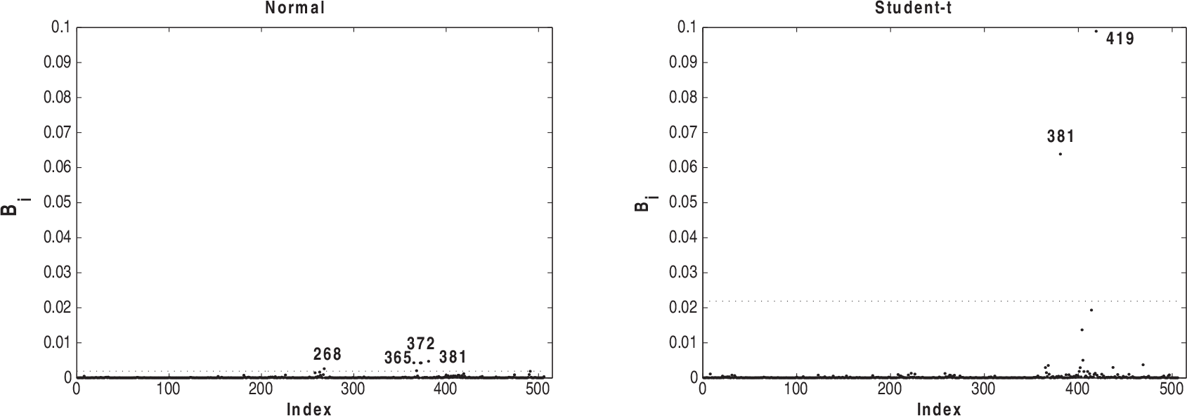
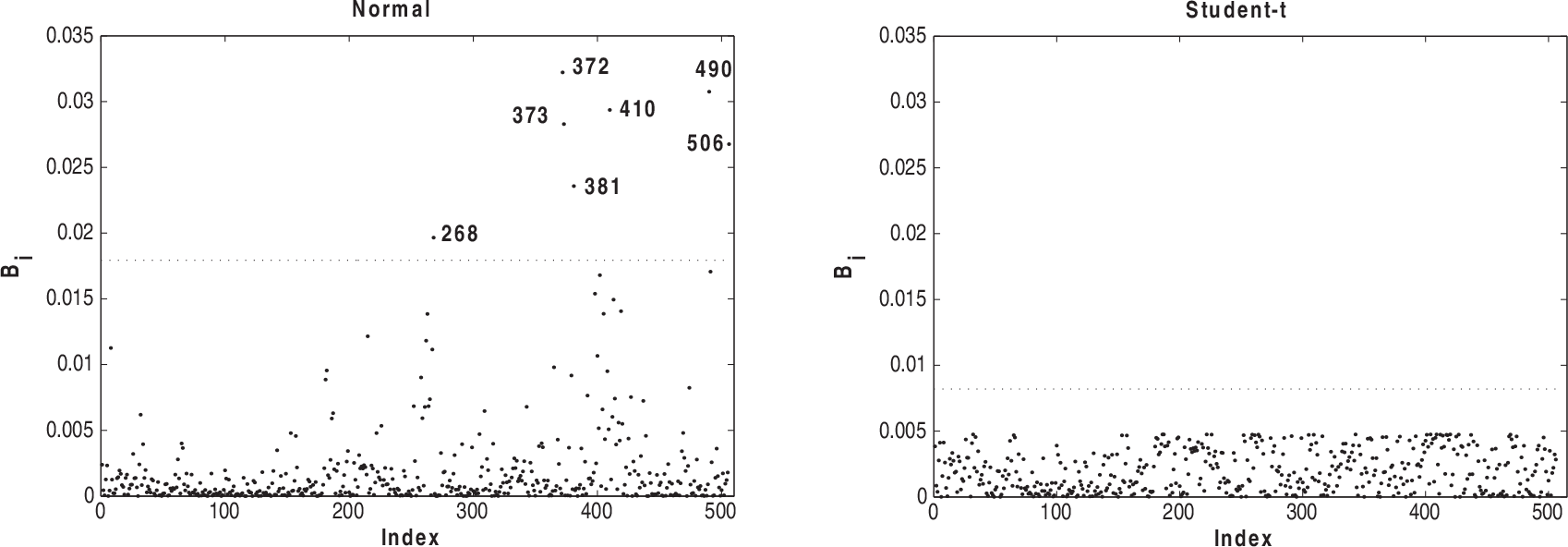
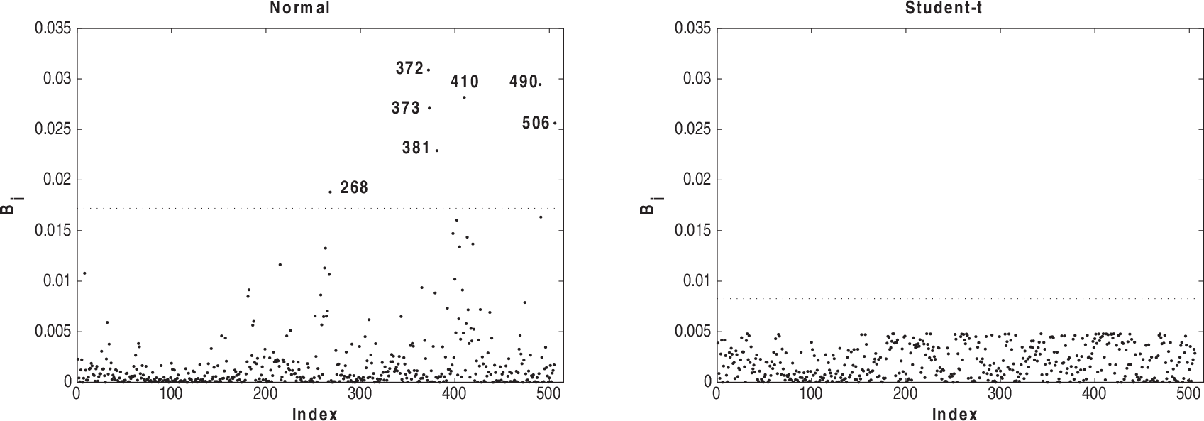
Index plots of B_i for assessing local influence on β₁ under case-weight perturbation for normal and Student-t models fitted to house prices data

Figure 7:

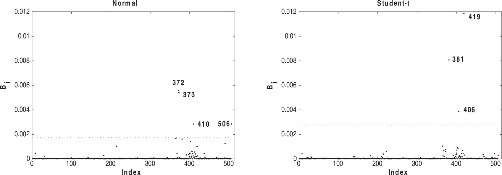
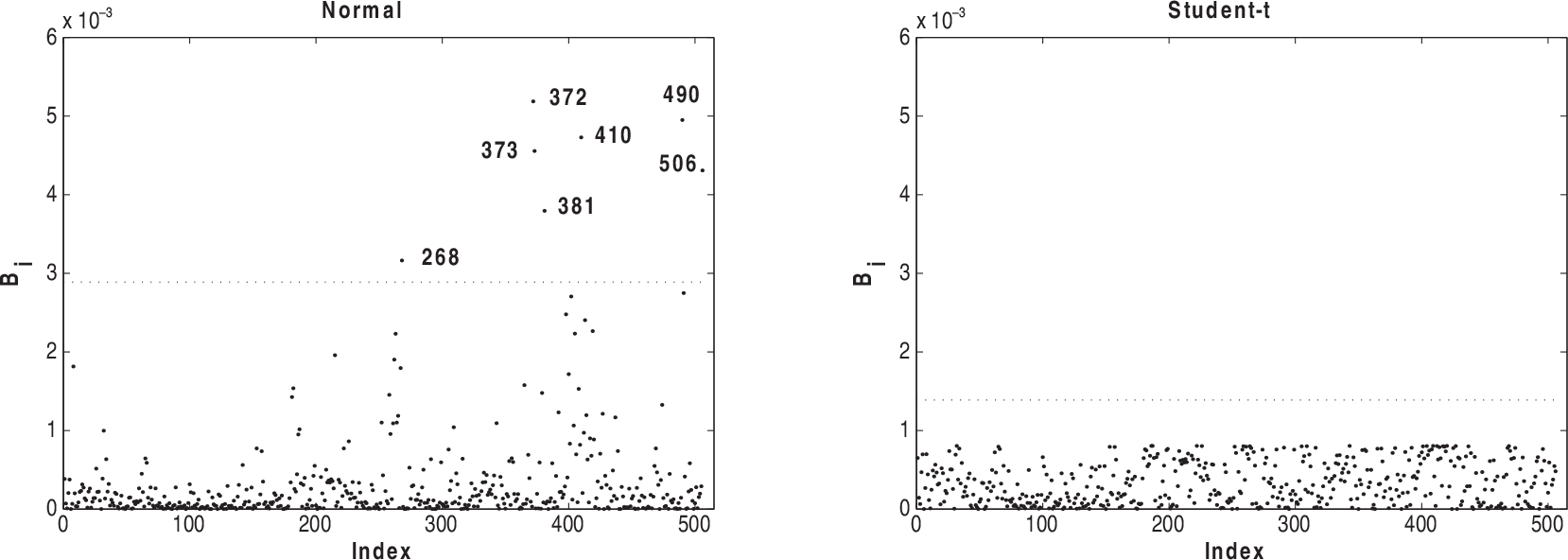
Index plots of B_i for assessing local influence on β₂ under case-weight perturbation for normal and Student-t models fitted to house prices data

6.2.1 Case-weight perturbation

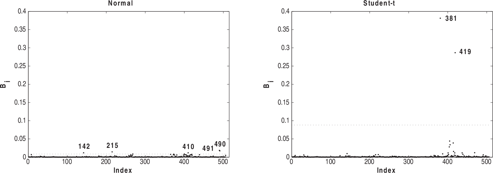
Figures 5–8 present the index plots of B_i for the case-weight scheme under the two fitted models. Considering Figure 5, we notice that 381, 365, 372, 268 and 369 are pointed out under the normal model and observations 419 and 381 have the greatest values under Student-t model. Based on Figure 6, we notice that observations 381, 419 and 405 are more influential under the normal model, whereas observations 405, 381 and 406 appear as influential under the Student-t model. Looking at Figure 7, we observe that the observations 490, 491, 215, 410 and 142 appear with a small influence under the normal model, whereas the observations 381 and 419 have the greatest influence under Student-t. From Figure 8, we notice that observations 372, 373, 410 and 506 are more influential under normal model and the observations 419, 381 and 406 have the greatest values under the Student-t model.

Figure 8:

Index plots of B_i for assessing local influence on ϕ under case-weight perturbation for normal and Student-t models fitted to house prices data

6.2.2 TAX perturbation

The index plots of $B_{i}$ under the TAX perturbation scheme are given in Figures 9–12. Considering Figures 9–12, we note that observations 372, 490, 410, 373, 506, 381 and 268 are more influential under normal model. However, no one observation is pointed out as influential under the Student-t model.

Figure 9:

Index plots of B_i for assessing local influence on α under TAX perturbation for normal and Student-t models fitted to house prices data

Figure 10:

Index plots of B_i for assessing local influence on β₁ under TAX perturbation for normal and Student-t models fitted to house prices data

Figure 11:

Index plots of B_i for assessing local influence on β₂ under TAX perturbation for normal and Student-t models fitted to house prices data

Figure 12:

Index plots of B_i for assessing local influence on ϕ under under TAX perturbation for normal and Student-t models fitted to house prices data

Based on these local influence graphics, we can conclude that the MPLEs for the regression coefficient $α$ and coefficient function $β_{2}$ appear to be less sensitive in the normal model under case-weight perturbation, whereas the sensitivity of ${\hat{β}}_{1}$ and $\hat{ϕ}$ appears to be similar under the two fitted models. Under TAX perturbation, the MPLE of the regression coefficient, coefficients functions and scale parameter from the Student-t model with 5 df appears to be less sensitive than the MPLE from the normal model. Note that 381 is pointed out in various graphics for the Student-t model.

7 Concluding remarks

In this article, we discuss parameter estimation and some statistical diagnostics for PVCM under elliptical errors. Local influence approaches for the proposed model under case-weight, scale parameter and explanatory variable perturbations are developed. Closed-form expressions are obtained for the penalized observed and expected information matrices. A real dataset previously analysed under normal errors is reanalysed under Student-t errors by assuming the smoothing parameter fixed and by applying the AIC to choose a df parameter estimate. The study provides evidences on the robust aspects of the MPLEs from Student-t PVCM with small df against outlying observations, as pointed out by Ibacache-Pulgar et al. (2013) in the context of symmetric semiparametric additive models. However, these robust aspects do not seem to be extended to all perturbation schemes of the local influence approach, indicating the usefulness of the normal curvatures derived in this article for assessing the sensitivity of the MPLEs from the elliptical PVCMs. Thus, we can recommend Student-t PVCMs as an option to fit symmetric datasets with partially varying-coefficient and indications of heavy tails. The codes in MATLAB used in the application may be obtained from the authors by request.

Acknowledgements

This work was supported by Project FONDECYT 11130704, Chile.

Appendix

A.1 Score function

Assuming that (3.3) is regular with respect to $α$ , $β_{k}$ ’s and $τ$ , the ( $p^{*} \times 1$ ) penalized score function vector of $θ$ is given by

U_{p} (θ) = \sum_{i = 1}^{n} \frac{\partial L_{p} (θ, λ)}{\partial θ} .

In particular, we obtain

\begin{matrix} \frac{\partial L_{p} (θ, λ)}{\partial α} & = & Z^{T} W_{v} r, \\ \frac{\partial L_{p} (θ, λ)}{\partial β_{k}} & = & {\tilde{N}}_{k}^{T} W_{v} r - λ_{k} K_{k} β_{k} (k = 1, \dots, s) \end{matrix}

and

\begin{matrix} \frac{\partial L_{p} (θ, λ)}{\partial τ_{ℓ}} & = & - \frac{1}{2} \sum_{i = 1}^{n} [tr (Σ_{i}^{- 1} \frac{\partial Σ_{i}}{\partial τ_{ℓ}}) - v_{i} r_{i}^{T} Σ_{i}^{- 1} \frac{\partial Σ_{i}}{\partial τ_{ℓ}} Σ_{i}^{- 1} r_{i}], \end{matrix}

where

r = (r_{1}^{T}, \dots, r_{n}^{T})^{T}

W_{v} = {blockdiag}_{1 \leq i \leq n} (v_{i} W_{i})

, with

W_{i} = Σ_{i}^{- 1}

v_{i} = - 2 ζ_{g} (δ_{i})

and

ζ_{g} (δ_{i}) = \frac{d \log g (δ_{i})}{d δ_{i}}

A.2 Hessian matrix

Let $L_{p}$ ( $p^{*} \times p^{*}$ ) be the Hessian matrix. The $(j^{*}, ℓ^{*})$ th element of $L_{p}$ , with respect to the parameters $θ_{j^{*}}$ and $θ_{ℓ^{*}}$ , is given by

L_{p} = \sum_{i = 1}^{n} \frac{\partial^{2} L_{p_{i}} (θ, λ)}{\partial θ_{j^{*}} \partial θ_{ℓ^{*}}} (j^{*}, ℓ^{*} = 1, \dots, p^{*}) .

For simplicity, let

Ψ_{i} = 2 Ψ_{1 i} + Ψ_{2 i}

Ψ_{i}^{*} = Ψ_{1 i} + Ψ_{2 i}

and

Ψ_{i}^{* *} = Ψ_{1 i} + 2 Ψ_{2 i}

, with

Ψ_{1 i} = v_{i}^{'} Σ_{i}^{- 1} r_{i} r_{i}^{T} Σ_{i}^{- 1}

and

Ψ_{2 i} = v_{i} Σ_{i}^{- 1}

. After some algebraic manipulations, we find

\begin{matrix} \frac{\partial^{2} L_{p_{i}} (θ, λ)}{\partial α \partial α^{T}} & = & - z_{i}^{T} Ψ_{i} z_{i}, \\ \frac{\partial^{2} L_{p_{i}} (θ, λ)}{\partial β_{k} \partial β_{k^{'}}^{T}} & = & \{\begin{matrix} - {\tilde{N}}_{ki}^{T} Ψ_{i} {\tilde{N}}_{ki} - \frac{λ_{k}}{n} K_{k} & k = k^{'} \\ - {\tilde{N}}_{ki}^{T} Ψ_{i} \tilde{N} k^{'} i & k \neq k^{'}, \end{matrix} \\ \frac{\partial^{2} L_{p_{i}} (θ, λ)}{\partial α \partial β_{k}^{T}} & = & - z_{i}^{T} Ψ_{i} {\tilde{N}}_{ki}, \\ \frac{\partial^{2} L_{p_{i}} (θ, λ)}{\partial α \partial τ_{J}} & = & - z_{i}^{T} Ψ_{i}^{*} \frac{\partial Σ_{i}}{\partial τ_{J}} Σ_{i}^{- 1} r_{i}, \\ \frac{\partial^{2} L_{p_{i}} (θ, λ)}{\partial β_{k} \partial τ_{J}} & = & - {\tilde{N}}_{ki}^{T} Ψ_{i}^{*} \frac{\partial Σ_{i}}{\partial τ_{J}} Σ_{i}^{- 1} r_{i} and \end{matrix}

\begin{matrix} \frac{\partial^{2} L_{p_{i}} (θ, λ)}{\partial τ_{J} \partial τ_{ℓ}} & = & \frac{1}{2} tr (Σ_{i}^{- 1} [\frac{\partial Σ i}{\partial τ_{ℓ}} Σ_{i}^{- 1} \frac{\partial Σ_{i}}{\partial τ_{J}} - \frac{\partial^{2} Σ_{i}}{\partial τ_{J} \partial τ_{ℓ}}]) - \frac{1}{2} r_{i}^{T} Σ_{i}^{- 1} \times \\ [\frac{\partial Σ i}{\partial τ ℓ} Ψ_{i}^{* *} \frac{\partial Σ_{i}}{\partial τ_{J}} - v_{i} \frac{\partial^{2} Σ_{i}}{\partial τ_{J} \partial τ_{ℓ}}] Σ_{i}^{- 1} r_{i}, \end{matrix}

where

v_{i}^{'} = \frac{d v_{i}}{d δ_{i}}

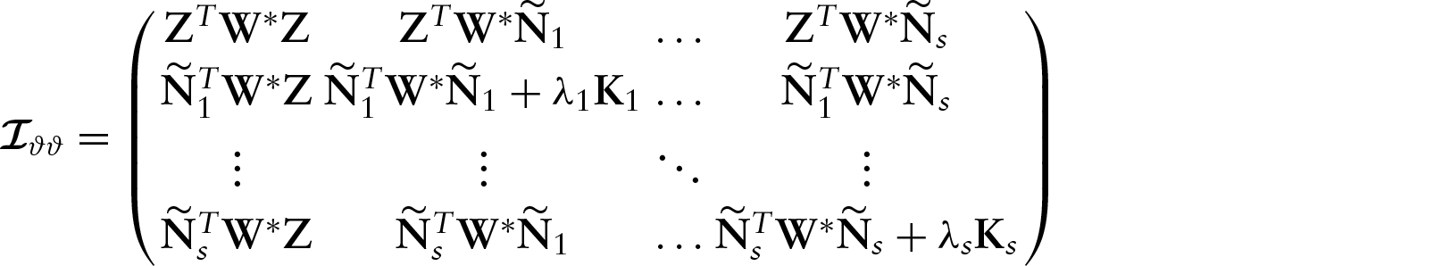
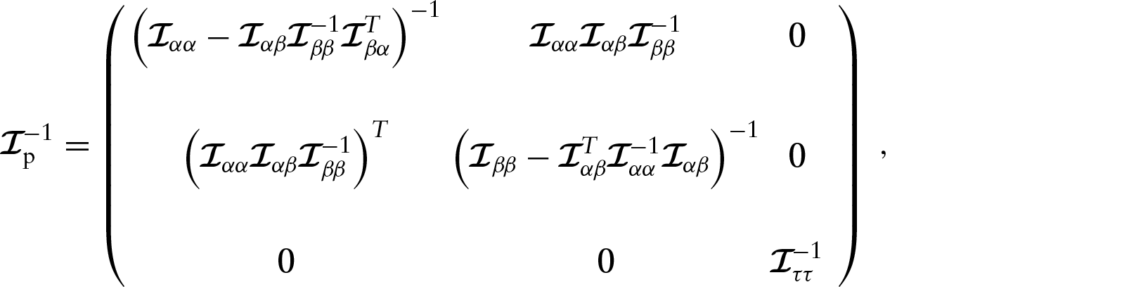
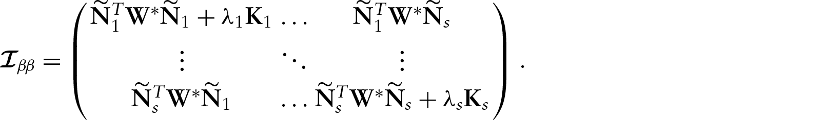
A.3 Expected information matrix

In general, by calculating the expectation of the matrix $- L_{p}$ , we obtain the ( $p^{*} \times p^{*}$ ) penalized expected information matrix, denoted by

\begin{matrix} ℐ_{p} & = & - E (\sum_{i = 1}^{n} \frac{\partial^{2} L_{p_{i}} (θ, λ)}{\partial θ_{j^{*}} \partial θ_{ℓ^{*}}}) . \end{matrix}

Following to Lange et al. (1989), we have that the

(j^{*}, ℓ^{*})

th element of the matrix

ℐ_{p}

for

i

th cluster, with respect to the parameters

θ_{j^{*}}^{*}

and

θ_{ℓ^{*}}^{*}

, can be obtained as

ℐ_{p_{i}} = E (\frac{\partial L_{p_{i}} (θ, λ)}{\partial θ_{j^{*}}} \frac{\partial L_{p_{i}} (θ, λ)}{\partial θ_{ℓ^{*}}}) .

Let $d_{g_{i}} = E (ζ_{g}^{2} (δ_{i}) δ_{i})$ and $f_{g_{i}} = E (ζ_{g}^{2} (δ_{i}) δ_{i}^{2})$ , with $δ_{i} = e_{i}^{T} e_{i}$ , $e_{i}$ $\sim$ ${El}_{m_{i}} (0, I_{m_{i}})$ , and $W^{*} = {blockdiag}_{1 \leq i \leq n} (\frac{4 d_{g_{i}}}{m_{i}} W_{i})$ . After some algebraic manipulations, we find

\begin{matrix} ℐ_{p} & = & blockdiag (I_{ϑ ϑ}, I_{τ τ}), \end{matrix}

where

\begin{matrix} ℐ_{ϑ ϑ} & = & (\begin{matrix} Z^{T} W^{*} Z & Z^{T} W^{*} {\tilde{N}}_{1} & \dots & Z^{T} W^{*} {\tilde{N}}_{s} \\ {\tilde{N}}_{1}^{T} W^{*} Z & {\tilde{N}}_{1}^{T} W^{*} {\tilde{N}}_{1} + λ_{1} K_{1} & \dots & {\tilde{N}}_{1}^{T} W^{*} {\tilde{N}}_{s} \\ ⋮ & ⋮ & ∺ & ⋮ \\ {\tilde{N}}_{s}^{T} W^{*} Z & {\tilde{N}}_{s}^{T} W^{*} {\tilde{N}}_{1} & \dots & {\tilde{N}}_{s}^{T} W^{*} {\tilde{N}}_{s} + λ_{s} K_{s} \end{matrix}) \end{matrix}

and

\begin{matrix} ℐ_{τ τ} & = & \sum_{i = 1}^{n} ℐ_{τ τ_{i}}, \end{matrix}

where the (

j, ℓ

)th element of

ℐ_{τ τ_{i}}

is given by

\begin{matrix} ℐ_{{jℓ}_{i}} & = & [\frac{b_{ℓ_{i}}}{4} (\frac{4 f_{g_{i}}}{m_{i} (m_{i} + 2)} - 1) + \frac{2 f_{g_{i}}}{m_{i} (m_{i} + 2)} tr (Σ_{i}^{- 1} \frac{\partial Σ_{i}}{\partial_{τ}} Σ_{i}^{- 1} \frac{\partial Σ_{i}}{\partial τ_{ℓ}})], \end{matrix}

where

b_{{jℓ}_{i}} = tr (Σ_{i}^{- 1} \frac{\partial Σ_{i}}{\partial_{τ}}) tr (Σ_{i}^{- 1} \frac{\partial Σ_{i}}{\partial τ_{ℓ}})

References

Akaike

(1973) Information theory and an extension ofthe maximum likelihood principle. In Petrov

Csàki

, International Symposium on Information Theory pages 267–81. Budapest: Akadémiai Kiadó

Belsley

Kuh

Welsch

(1980) Regression Diagnostics: Identifying Influential Data and Sources of Collinearity . New York, NY: Wiley.

Berhane

Tibshirani

(1998) Generalized additive models for longitudinal data. The Canadian Journal of Statistics , 26, 517–35.

Cook

(1986) Assessment of local influence (with discussion). Journal of the Royal Statistical Society B , 48, 133–69.

Craven

Wahba

(1979) Smoothing noisy data with spline functions. Numerical Mathematical , 31, 377–403.

Eilers

PHC

Marx

(1996) Flexible smoothing with B-splines and penalties. Statistical Science , 11, 89–121.

Díaz-Garcia

Galea

Leiva-Sanchez

(2003) Influence diagnostics for elliptical multivariate linear regression models. Communications in Statistics, Theory and Methods , 32, 625–41.

Fang

Kotz

(1990) Symmetric Multivariate and Related Distribution . London: Chapman and Hall.

Fung

Zhu

Wei

(2002) Influence diagnostics and outlier tests for semiparametric mixed models. Journal of the Royal Statistical Society B , 64, 565–79.

10.

Galea

Paula

Bolfarine

(1997) Local influence in elliptical linear regression models. The Statistician , 46, 71–9.

11.

Galea

Paula

Cysneiros

FJA

(2005) On diagnostics in symmetrical nonlinear models. Statistics and Probability Letters , 73, 459–67.

12.

Green

(1987) Penalized likelihood for general semi-parametric regression models. International Statistical Review , 55, 245–59.

13.

Green

Silverman

(1994) Nonparametric Regression and Generalized Linear Models . Boca Raton: Chapman and Hall.

14.

Gourieroux

Monford

(1995) Statistics and Econometric Models , Vols. 1 and 2. Cambridge: Cambridge University Press.

15.

Harrison

Rubinfeld

(1978) Hedonic housing prices and the demand for clean air. Journal of Environmental Economics and Management , 5, 81–102.

16.

Hastie

Tibshirani

(1990) Generalized Additive Models . London: Chapman and Hall.

17.

Hastie

Tibshirani

(1993) Varying-coefficient models. Journal of the Royal Statistical Society B , 55, 757–96.

18.

Hurvich

Simonoff

Tsai

(1998) Smoothing parameter selection in nonparametric regression using an improved Akaike information criterion. Journal of the Royal Statistical Society B , 60, 271–93.

19.

Ibacache-Pulgar

Paula

(2011) Local influence for Student-t partially linear models. Computational Statistics and Data Analysis , 55, 1462–78.

20.

Ibacache-Pulgar

Paula

Galea

(2012) Influence diagnostics for elliptical semiparametric mixed models. Statistical Modelling , 12, 165–93.

21.

Ibacache-Pulgar

Paula

Cysneiros

FJA

(2013) Semiparametric additive models under symmetric distributions. Test , 22, 103–21.

22.

Kim

Park

Kim

(2002) Influence diagnostics in semiparametric regression models. Statistics and Probability Letters , 60, 49–58.

23.

Lange

Little

RJA

Taylor

JMG

(1989) Robust statistical modelling using the t distribution. Journal of the American Statistical Association , 84, 881–96.

24.

Zhu

(2009) Influence diagnostics and outlier test for varying coefficient mixed models. Journal of Multivariate Analysis , 100, 2002–17.

25.

Paula

Cysneiros

FJA

Galea

(2003) Local Influence and Leverage in Elliptical Nonlinear Regression Models. In Verbeke

Molenberghs

Aerts

Fieuws

Proceedings of the 18th International Workshop on Statistical Modelling , pages 361–65. Leuven: Katholieke Universiteit Leuven.

26.

Poon

(1999) Conformal normal curvature and assessment of local influence. Journal of the Royal Statistical Society B , 61, 51–61.

27.

Rigby

Stasinopoulos

(2005) Generalized additive models for location, scale and shape. Applied Statistics , 54, 507–54.

28.

Simonoff

Tsai

(1999) Semiparametric and additive model selection using an improved Akaike information criterion. Journal of Computational and Graphical Statistics , 8, 22–40.

29.

Thomas

(1991) Influence diagnostics for the cross-validated smoothing parameter in spline smoothing. Journal of the American Statistical Association , 86, 693–98.

30.

Wei

(2004) Derivatives diagnostics and robustness for smoothing splines. Computational Statistics and Data Analysis , 46, 335–56.

31.

Zhang

Zhiya

(2015) Local influence analysis of varying coefficient linear model. Journal of Interdisciplinary Mathematics , 3, 293–306.

32.

Zhu

Fung

(2003) Local influence analysis for penalized Gaussian likelihood estimators in partially linear models. Scandinavian Journal of Statistics , 30, 767–80.

Local influence for elliptical partially varying-coefficient model

Abstract

Keywords

1 Introduction

2 Motivating example

Figure 1:

Scatter plots: LMV versus TAX (a), LMV versus LSTAT, (b) LMV versus ROOM × LSTAT (c) and CRIM × LSTAT (d)

Index plots of the Mahalanobis distance under normal (a) and Student-t (b) models and between the estimated weights and Mahalanobis distance under Student-t model (c)

3.1 The model

3.3 Penalized function

4.1 Maximizing the penalized log-likelihood function

4.2 Fisher score and weighted back-fitting algorithms

4.4 Approximate standard errors

4.6 On degrees of freedom

5 Local influence measure

5.1 The method

5.2 Conformal normal curvature

5.3 Normal curvature derivation

5.3.1 Case-weight perturbation

5.3.3 Explanatory variable perturbation

Table 1:

MPLEs, estimated standard errors and AIC values under normal and Student-t ( ν = 5 ) models fitted to house prices data

Plots of estimated coefficient functions for the house prices data, and their approximate pointwise SEB denoted by the dashed lines

Scatter plots of LMV versus fitted LMV: normal (a) and Student-t models (b)

Figure 5:

Index plots of B i for assessing local influence on α under case-weight perturbation for normal and Student-t models fitted to house prices data

Index plots of B i for assessing local influence on β1 under case-weight perturbation for normal and Student-t models fitted to house prices data

Index plots of B i for assessing local influence on β2 under case-weight perturbation for normal and Student-t models fitted to house prices data

Figure 8:

Index plots of B i for assessing local influence on ϕ under case-weight perturbation for normal and Student-t models fitted to house prices data

Figure 9:

Index plots of B i for assessing local influence on α under TAX perturbation for normal and Student-t models fitted to house prices data

Index plots of B i for assessing local influence on β1 under TAX perturbation for normal and Student-t models fitted to house prices data

Index plots of B i for assessing local influence on β2 under TAX perturbation for normal and Student-t models fitted to house prices data

Index plots of B i for assessing local influence on ϕ under under TAX perturbation for normal and Student-t models fitted to house prices data

Acknowledgements

A.1 Score function

A.2 Hessian matrix

A.3 Expected information matrix

References

MPLEs, estimated standard errors and AIC values under normal and Student-t ( $ν = 5$ ) models fitted to house prices data

Index plots of B_i for assessing local influence on α under case-weight perturbation for normal and Student-t models fitted to house prices data

Index plots of B_i for assessing local influence on β₁ under case-weight perturbation for normal and Student-t models fitted to house prices data

Index plots of B_i for assessing local influence on β₂ under case-weight perturbation for normal and Student-t models fitted to house prices data

Index plots of B_i for assessing local influence on ϕ under case-weight perturbation for normal and Student-t models fitted to house prices data

Index plots of B_i for assessing local influence on α under TAX perturbation for normal and Student-t models fitted to house prices data

Index plots of B_i for assessing local influence on β₁ under TAX perturbation for normal and Student-t models fitted to house prices data

Index plots of B_i for assessing local influence on β₂ under TAX perturbation for normal and Student-t models fitted to house prices data

Index plots of B_i for assessing local influence on ϕ under under TAX perturbation for normal and Student-t models fitted to house prices data