Improved local quantile regression

Abstract

We investigate a new kernel-weighted likelihood smoothing quantile regression method. The likelihood is based on a normal scale-mixture representation of asymmetric Laplace distribution (ALD). This approach enjoys the same good design adaptation as the local quantile regression (Spokoiny et al., 2013, Journal of Statistical Planning and Inference, 143, 1109–1129), particularly for smoothing extreme quantile curves, and ensures non-crossing quantile curves for any given sample. The performance of the proposed method is evaluated via extensive Monte Carlo simulation studies and one real data analysis.

Keywords

Bandwidth selection asymmetric Laplace distribution non-parametric quantile regression propagation condition quantile crossing

Introduction

Parametric quantile regression (Koenker, 2005) has been used in a number of disciplines to explore the relationship between the response and covariates at both the centre and extremes of the conditional distribution and obtain a more comprehensive analysis of the relationship between variables. While a parametric model is possibly misspecified, non-parametric models, on the other hand, require fewer assumptions about the data and offer a more flexible way of modelling a relationship than parametric models, consequently avoid model misspecification when a parametric model is not available, which is common in wide applications (wand, 1995; fan, 1996; takezawa, 2005). One of the popular non-parametric smoothing techniques is kernel smoothing. Non-parametric kernel smoothing quantile regression has attracted much attention in the literature (Chaudhuri, 1991; Hardle, 1993; fan, 1996; Yu, 1998; Cai, 2008; Dette, 2008; Dabo-Niang, 2012; Schaumburg, 2012; Kong, 2017).

However, the performance of kernel smoothing techniques, in spite of their advantages over parametric models in dealing with model misspecification, depends on smoothing parameter or bandwidth selection. While a global bandwidth such as the rule of thumb (Yu, 1998) is generally useful, a point-wise bandwidth, which depends on the values of covariate $X$ or the design set should be considered for the complexity of the underlying regression functions. In particular, bandwidth selection in non-parametric smoothing quantile regression requires not only design adaptation but also quantile adaptation. Spokoiny, Wang and H $\ddot{a}$ rdle (henceforth SWH) (Spokoiny, 2014) developed a kernel-weighted likelihood quantile regression with point-wise bandwidth selection and promising performance in practice.

But SWH's approach may not guarantee non-crossing quantile curves for any given sample (calculated for various percentile $τ \in (0, 1))$ , which is a common problem in the estimation of conditional and structural quantile functions due to lack of monotonicity. Note that monotonicity (for each $x$ in the design set, it is a monotone function of percentile value $τ$ ) guarantees non-crossing quantile curves, but not vice versa. Such a phenomenon violates the basic principle of probability theory, that is, the associated distribution functions should be monotone increasing. Various methods were presented to address or avoid the quantile crossing in parametric quantile regression, but with few on non-parametric quantile regression. Recently, (Jones, 2007) improved double kernel smoothing for quantile regression; (Bondell, 2010) and (muggeo, 2013) used spline-based constraints to incorporate non-crossing conditions; (qu, 2015) applied inequality constrains to ensure the monotonicity over quantiles; and (liu, 2011) dealt with this issue via simultaneous multiple quantile smoothing.

In this article, we explore a local likelihood-based quantile regression based on a normal scale-mixture (NSM) representation of asymmetric Laplace distribution (ALD) and show that this method has the similar property of SWH's procedure but a much better adaptation for smoothing extreme quantile curves. Moreover, a theoretical justification of the estimated non-crossing quantile curves, that is, estimated quantile function is monotone with respect to $τ$ for all $x$ , is given by our proposed method. Therefore, the proposed method enjoys both design adaptation and non-crossing quantile curves simultaneously. This article is organized as follows. We first review SWH's approach in Section 2, then propose a new local likelihood smoothing based on an NSM representation of ALD and show that this approach satisfies the propagation condition (PCs Spokoiny, 2009) in Section 3. In Section 4 we elaborate the proposed adaptive bandwidth selection rule and point out that the rule is able to avoid the problem of quantile curves crossing, especially for estimating extreme quantiles. Section 5 illustrates the numerical performance of the proposed method. Section 6 provides concluding remarks and discusses future work.

Kernel-weighted likelihood for local quantile regression

(Spokoiny, 2014) developed an interesting non-parametric quantile regression method: local quantile regression, which provides point-wise bandwidth selection and exhibits promising performance in practice. SWH claimed that their bandwidth selection rule is adaptive and novel, although the regression estimator named qMLE in their Equation (8) is simply equivalent to a local polynomial quantile regression or a type of kernel-based weighting ‘check function’ approach, such as the local linear single-kernel approach of Yu, 1998.

Let $(X, Y)$ be the random variables, where $Y$ is a continuous random variable and $X$ is a univariate regressor $X \in 𝕣^{1}$ . Let $F_{Y} (Y | X)$ be the cumulative distribution function of $Y$ given $X$ . Let $Q_{τ} (Y | X) = inf \{Y : F_{Y} (Y | X) \geq τ\}$ be the inverse function, which is also the value of $a$ that minimizes the expected loss function:

Q_{τ} (Y | X) = \underset{a}{argmin} E ρ_{τ} (Y - a),

(2.1)

where, $τ \in (0, 1)$ and $ρ_{τ} (\cdot)$ is an asymmetric loss function that satisfies $ρ_{τ} (u) = u (τ - I (u < 0))$ where $I (\cdot)$ is an indicator function.

Under the quantile non-parametric model $Y = f (X) + ε$ , given data in the form ${X_{i}, Y_{i}}_{i = 1}^{n}$ , where $X_{i}$ and $Y_{i}$ are independent scalar observations of $X$ and $Y$ , respectively. The $τ$ th conditional quantile of $Y$ given $X$ is estimated by

\hat{f} (x) = \underset{β}{argmin} \sum_{i = 1}^{n} ρ_{τ} (Y_{i} - f (X_{i})) .

(2.2)

SWH took advantage of the link between the minimization of the sum of the loss function in Equation (2.2) and the maximum likelihood method based on an ALD. For a random variable $Y \sim ALD (μ, σ, τ)$ , its density function can be written as

f (y; μ, σ, τ) = \frac{τ (1 - τ)}{σ} exp \{\frac{y - μ}{σ} [τ - I (y \leq μ)]\}, ​ ​ ​ ​ y \in (- \infty, + \infty),

(2.3)

where $0 < τ < 1$ is skew parameter, $σ > 0$ is scale parameter and $- \infty < μ < \infty$ is location parameter.

Based on an ALD log-likelihood, SWH considered

L_{SWH} (θ) \equiv log \{τ (1 - τ)\} \sum_{i = 1}^{n} I - \sum_{i = 1}^{n} ρ_{τ} (Y_{i} - f_{θ} (X_{i})),

(2.4)

where $0 < τ < 1$ is the level of the quantile. Then they fit $f (x)$ at point $x$ by the local polynomial approach $Y_{i} = ψ_{i}^{T} θ + ε$ , with basis $ψ_{i} = {1, (X_{i} - x), (X_{i} - x)^{2} / 2!, \dots, (X_{i} - x)^{p} / p!}^{T}$ and $θ = (θ_{0}, . . ., θ_{p})^{T}$ . Therefore, the local log-likelihood at $x$ is given by

L_{SWH} (W, θ) \equiv log τ (1 - τ) \sum_{i = 1}^{n} w_{i} - \sum_{i = 1}^{n} ρ_{τ} (Y_{i} - ψ_{i}^{T} θ) w_{i},

(2.5)

where the weights $W$ is chosen via a kernel function $w_{i} = K (\frac{X_{i} - x}{h})$ , while $h$ is a bandwidth controlling the degree of localization. Note that Equation (2.5) is similar to the global log-likelihood in Equation (2.4), but each summand in $L_{SWH} (W, θ)$ is multiplied with the weight $w_{i}$ , so only the points from the local vicinity of $x$ contribute to $L_{SWH} (W, θ)$ .

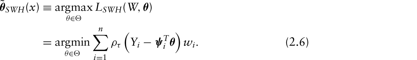
The corresponding local quantile MLE (they named it as qMLE) at $x$ is then given via the maximization of $L_{SWH} (W, θ)$ in Equation (2.4)

\begin{matrix} {\tilde{θ}}_{SWH} (x) & \equiv & \underset{θ \in Θ}{argmax} L_{SWH} (W, θ) \\ = & \underset{θ \in Θ}{argmin} \sum_{i = 1}^{n} ρ_{τ} (Y_{i} - ψ_{i}^{T} θ) w_{i} . \end{matrix}

(2.6)

3 Local quantile regression with an alternative likelihood for smoothing

Figure 1a displays the performance of SWH's approach, showing the bandwidth sequence (upper panel) and the smoothed 50% quantile curve (lower panel) based on the Lidar dataset (available in R package SemiPar), which adapts the data well. And this is also true for other moderate or central quantile curves. However, it can be seen from smoothing extreme quantile curves in Figure 1 that the proposed bandwidth selection rule lacks good adaptation and then results in the over-smoothing phenomenon. Figures 1b and 1c display the smoothed 1% and 99% quantile curves using SWH's method and show that when the curves start to switch smoothness, the rule is not adaptive so that the estimated curves are too smoothing out of the data ranges. A possibly theoretical interpretation for this problem is: when $τ \to 0$ , the weighted ‘check function’ $ρ_{τ} (Y_{i} - ψ_{i}^{T} θ) w_{i}$ takes constant 0, if $Y_{i} > ψ_{i}^{T} θ$ (also, when $τ \to 1$ and if $Y_{i} < ψ_{i}^{T} θ$ ). This may result in that the proposed significant test always picks constant bandwidth for smoothing extreme quantile curves, although this is not a problem for the local quantile regression estimation equation. We want to point out that this over-smoothing problem will be solved by a new version of adaptive bandwidth selection rule.

Figure 1:

The bandwidth sequences (upper panels) and smoothed quantile curves (lower panels) for the Lidar dataset using SWH's kernel-weighted likelihood

Moreover, there is no guaranteed of this approach to avoid quantile crossing. Therefore, we propose an alternative adaptive bandwidth selection rule based on a NSM representation of ALD and show that this alternative version has the similar property to SWH's procedure but much better-adaptation for smoothing extreme quantile curves.

(Reed, 2010) and (Kozumi, 2011) noted that under the assumption of ALD-based ‘working likelihood’, the quantile regression model error $ε \sim ALD (0, 1, τ)$ can be represented as a scale mixture of normal variables, that is,

ε = μ z + δ \sqrt{z} e,

(3.1)

where $μ = \frac{1 - 2 τ}{τ (1 - τ)}$ , $δ^{2} = \frac{2}{τ (1 - τ)}$ , $z \sim Exp (1)$ and $e \sim N (0, 1)$ , and $z$ and $e$ are independent. Hence, SWH's model (1) $(Y_{i} = f (X_{i}) + ε_{i})$ could be re-written as

Y_{i} = f (X_{i}) + μ z_{i} + δ \sqrt{z_{i}} e_{i} .

(3.2)

That is, for given $z = (z_{1}, z_{2}, \dots, z_{n})$ ,

Y_{i} \sim N (f (X_{i}) + μ z_{i}, δ^{2} z_{i}),

(3.3)

that is, the joint conditional density of $Y = (Y_{1}, Y_{2}, \dots, Y_{n})$ is given by

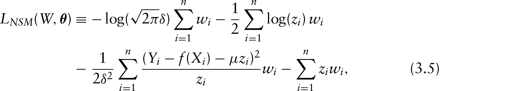
l (Y | z, X) = \prod_{i = 1}^{n} \frac{1}{\sqrt{2 π} δ \sqrt{z_{i}}} exp \{- \frac{{(Y_{i} - f (X_{i}) - μ z_{i})}^{2}}{2 δ^{2} z_{i}}\} .

(3.4)

Clearly, if $z$ is fixed in advance, then the local log-likelihood (SWH's Equation (7)) can be replaced by a NSM representation of ALD:

\begin{matrix} L_{NSM} (W, θ) & \equiv & - log (\sqrt{2 π} δ) \sum_{i = 1}^{n} w_{i} - \frac{1}{2} \sum_{i = 1}^{n} log (z_{i}) w_{i} \\ - & \frac{1}{2 δ^{2}} \sum_{i = 1}^{n} \frac{(Y_{i} - f (X_{i}) - μ z_{i})^{2}}{z_{i}} w_{i} - \sum_{i = 1}^{n} z_{i} w_{i}, \end{matrix}

(3.5)

where the weights $W$ is chosen via a kernel function $w_{i} = K (\frac{X_{i} - x}{h})$ , while $h$ is a bandwidth controlling the degree of localization. Similar to Equation (2.5), the local log-likelihood in Equation (3.5) depends on the central point $x$ via the structure of the basis vectors $ψ_{i}$ and via the weights $w_{i}$ .

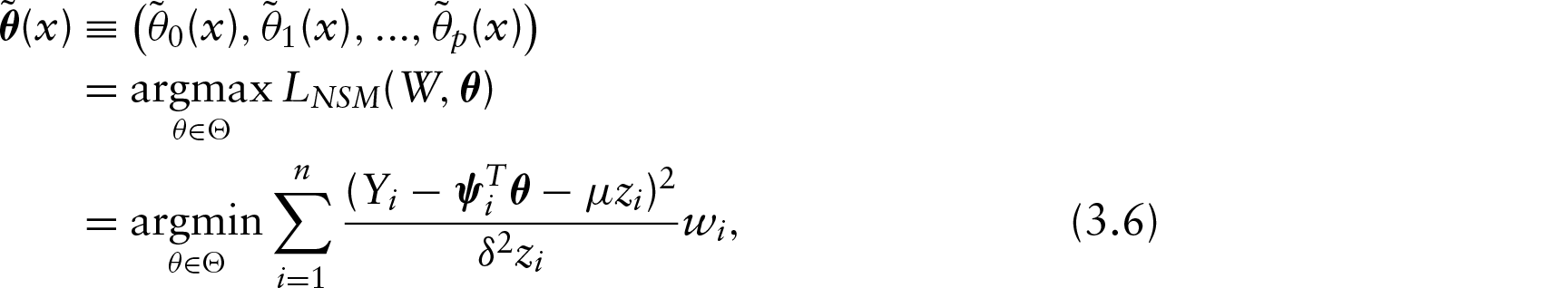
Now, once a local $p$ th-degree polynomial $ψ_{i}^{T} θ$ is used to approximate $f (x)$ at $X = x$ , the corresponding local qMLE at $x$ could be defined via maximization of $L_{NSM} (W, θ)$ earlier:

\begin{matrix} \tilde{θ} (x) & \equiv & ({\tilde{θ}}_{0} (x), {\tilde{θ}}_{1} (x), . . ., {\tilde{θ}}_{p} (x)) \\ = & \underset{θ \in Θ}{argmax} L_{NSM} (W, θ) \\ = & \underset{θ \in Θ}{argmin} \sum_{i = 1}^{n} \frac{(Y_{i} - ψ_{i}^{T} θ - μ z_{i})^{2}}{δ^{2} z_{i}} w_{i}, \end{matrix}

(3.6)

where ${\tilde{θ}}_{0} (x)$ estimates $f (x)$ , and ${\tilde{θ}}_{m} (x)$ estimates the $m^{th}$ derivative of $f (x)$ . Further, let $ψ = (ψ_{1}, \dots, ψ_{n})^{T}$ and $w_{k} = diag (\frac{w_{1}^{(k)}}{δ^{2} z_{1}}, . . ., \frac{w_{n}^{(k)}}{δ^{2} z_{n}})$ , we have

{\tilde{θ}}_{k} (x) = {({ψ w}_{k} ψ^{T})}^{- 1} {ψ w}_{k} (Y + μ z + δ z^{1 / 2} e),

(3.7)

where the design matrix $ψ$ consists of the columns $ψ_{i} = {1, (X_{i} - x), \dots, (X_{i} - x)^{p} / p!}^{T}$ .

We note that the $L_{NSM} (W, θ)$ involves in a specification of vector $z$ , and we point out that $z$ could be fixed in advance via a sample from a data-driven inverse Gaussian distribution, and our extensive experiments in Section 5 show that the selection of the sample has no effect on the estimation. In fact, note that the joint likelihood function of $(Y, z)$ is given by

f (Y, z | X) = \prod_{i = 1}^{n} \frac{1}{\sqrt{2 π} τ \sqrt{z_{i}}} exp \{- \frac{{(Y_{i} - f (X_{i}) - μ z_{i})}^{2}}{2 τ^{2} z_{i}}\} \prod_{i = 1}^{n} exp (- z_{i}) .

Therefore, the conditional density of $f (z | Y)$ is given by

\begin{matrix} f (z | Y) & \propto & f (Y, z) \\ \propto & \prod_{i = 1}^{n} \frac{1}{\sqrt{z_{i}}} exp (- \frac{1}{2} [\frac{{(Y_{i} - f (X_{i}))}^{2}}{δ^{2}} z_{i}^{- 1} + (\frac{μ^{2}}{δ^{2}} + 2) z_{i}]) . \end{matrix}

(3.8)

That is, $z_{i}, z_{2}, \dots, z_{n}$ are i.i.d. with a generalized inverse Gaussian (GIG) distribution:

\begin{matrix} f (z | Y) & \propto & z_{i}^{- \frac{1}{2}} exp (- \frac{1}{2} [\frac{{(Y_{i} - f (X_{i}))}^{2}}{δ^{2}} z_{i}^{- 1} + (\frac{μ^{2}}{δ^{2}} + 2) z_{i}]) \\ \sim & GIG (\frac{1}{2}, η_{i}, ζ_{i}), \end{matrix}

(3.9)

where $η_{i}^{2} = \frac{{(Y_{i} - f (X_{i}))}^{2}}{δ^{2}}$ and $ζ_{i}^{2} = \frac{μ^{2}}{δ^{2}} + 2$ .

4 Performance of adaptive bandwidth selection and non-crossing estimation

4.1 Adaptive bandwidth selection

There are several methodologies for automatic smoothing parameter selection. One class of methods chooses the smoothing parameter value to minimize a criterion that incorporates both the tightness of the fit and model complexity. Such a criterion can usually be written as a function of the error mean square, and a penalty function designed to decrease with increasing smoothness of the fit. Examples of specific criteria are generalized cross-validation (Craven, 1979) and the Akaike information criterion (AIC)(Akaike, 1973). These classical selectors have two undesirable properties when used with local polynomial and kernel estimators: they tend to under-smooth and tend to be non-robust in the sense that small variations in the input data can change the choice of smoothing parameter value significantly. (Hurvich, 1998) obtained several bias-corrected AIC criteria that limit these unfavourable properties and perform comparably with the plug-in selectors (Ruppert, 1995).

The adaptive bandwidth selection rule in SWH's paper is different from the rule of thumb of (Yu, 1998) and AIC rule of (Cai, 2008). It does add a nice option to the bandwidth selection menu for practitioners. In this article, we perform the local quantile curve estimation following the similar bandwidth selection procedures, but based on a NSM representation of ALD.

First, we fix a finite ordered set of candidates of bandwidth $h_{1} < h_{2} < \dots < h_{K}$ , where $h_{1}$ is very small. According to SWH, the bandwidth sequence can be taken geometrically increasing of the form $h_{k} = {ab}^{k}$ with fixed $a > 0$ , $b > 1$ , and $n^{- 1} < {ab}^{k} < 1$ for $k = 1, \dots, K$ . For each $k \leq K$ , an ordered weighting scheme $W^{(k)} = (w_{1}^{(k)}, w_{2}^{(k)}, \dots, w_{n}^{(k)})$ is chosen via a kernel function $w_{i}^{(k)} = K (\frac{X_{i} - x}{h_{k}})$ leading to the local quantile estimator at $x$ , ${\tilde{θ}}_{k} (x)$ , as:

\begin{matrix} {\tilde{θ}}_{k} (x) & = & \underset{θ \in Θ}{argmax} L_{NSM} (W^{(k)}, θ) \\ = & \underset{θ \in Θ}{argmin} \sum_{i = 1}^{n} \frac{(Y_{i} - ψ_{i}^{T} θ - μ z_{i})^{2}}{δ^{2} z_{i}} w_{i}^{(k)} . \end{matrix}

(4.1)

Then, we start with the smallest bandwidth $h_{1}$ . For any $k > 1$ , compute the local qMLE ${\tilde{θ}}_{k} (x)$ and check whether it is consistent with all the previous estimators ${\tilde{θ}}_{l} (x)$ for $l < k$ . We use a localized likelihood ratio test, that is, the difference $L_{NSM} (W^{(l)}, {\tilde{θ}}_{l} (x)) - L_{NSM} (W^{(l)}, {\tilde{θ}}_{k} (x))$ to reject ${\tilde{θ}}_{k} (x)$ , where ${\tilde{θ}}_{l} (x)$ maximize the log-likelihood $L_{NSM} (W^{(l)}, {\tilde{θ}}_{l} (x)) = sup_{θ} L_{NSM} (W^{(l)}, θ)$ defined in Equation (3.5) where bandwidth $h_{l}$ and $L_{NSM} (W^{(l)}, {\tilde{θ}}_{k} (x))$ is the other local likelihood under ${\tilde{θ}}_{k} (x)$ with bandwidth $h_{k} (l < k)$ . The difference checks whether ${\tilde{θ}}_{k} (x)$ belongs to the confidence set $ε_{l} (ζ)$ of ${\tilde{θ}}_{l} (x)$ :

ε_{l} (ζ) : = \{θ \in Θ : L_{NSM} (W^{(l)}, {\tilde{θ}}_{l} (x)) - L_{NSM} (W^{(l)}, {\tilde{θ}}_{k} (x)) \leq ζ_{l}\} .

If the consistency check is negative, the procedure terminates and selects the latest accepted estimator.

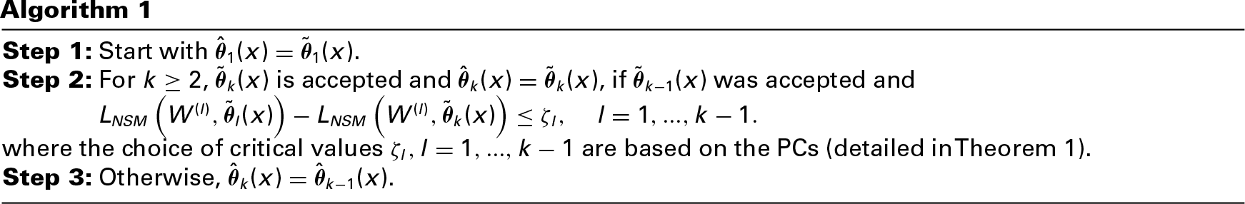
The adaptation algorithm can be summarized as follows:

The adaptive estimator $\hat{θ} (x)$ is the latest accepted estimator after all $K$ steps:

\hat{θ} (x) = {\hat{θ}}_{K} (x) .

Moreover, all the estimators ${\tilde{θ}}_{k} (x)$ should be consistent to each other and the procedure should not terminate at any intermediate step $k < K$ . This effect is called as ‘propagation’. Hence, under the assumptions (A1)–(A3) in Appendix, and then according to (Serdyukova, 2012), the propagation conditions (PCs) for this approach also satisfies:

Theorem 1. (Theoretical choice of the critical values.) Assume (A1)–(A3), given $α \in (0, 1]$ and $r > 0$ , the critical values $ζ_{1}, \dots, ζ_{K}$ satisfy

𝔼 {|{({\tilde{θ}}_{k} (x) - {\hat{θ}}_{k} (x))}^{T} (ψ w_{k} (x) ψ^{T}) ({\tilde{θ}}_{k} (x) - {\hat{θ}}_{k} (x))|}^{r} \leq α C (p, r),

(4.2)

for all $k = 2, \dots, K$ , where $C (p, r) = 2^{r} Γ (r + p / 2) / Γ (p / 2)$ , with the choice of the critical values of the form

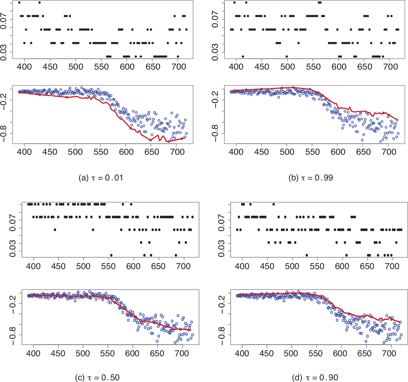
\begin{matrix} ζ_{l} = \frac{4}{μ} \{r (K - l) \log b + \log \frac{K}{α} - \frac{p}{4} \log (1 - 4 μ) - \log (1 - b^{- r}) + \overset{̅}{C} (p, r)\}, \\ l = 1, . . ., k - 1, \end{matrix}

where $μ \in (0, 1 / 4)$ is an arbitrary constant, $b > 1$ and $\overset{̅}{C} (p, r) = \log \{\frac{2^{2 r} {[Γ (2 r + p / 2) Γ (p / 2)]}^{1 / 2}}{Γ (r + p / 2)}\}$ . The critical values are selected to ensure the desired PCs which effectively means a ‘no alarm’ property, that is, the selected adaptive estimator coincides in the most cases that the estimator ${\tilde{θ}}_{k} (x)$ corresponding to the largest bandwidth. An advantage of the proposed alternative normal scale-mixture likelihood function over SWH's method is that the derived bandwidth has better adaptation when $τ$ tends to 0 or 1. Figure 2 displays the bandwidth sequence (upper panel) and smoothed quantile curves for quantiles 1% (2a) and 99% (2b) based on the Lidar dataset, which provides much better fitting than those curves presented in Figure 1. The dependency structure changing on smoothness is more adaptive than the bandwidth sequence in Figure 1. This alternative normal scale-mixture likelihood method also works well for other moderate or central quantile curves. Figure 2 shows that the method gives quite similar estimates to SWH's method for $τ = 0.5$ (2c) and $0.9$ (2d) quantile curves.

Figure 2:

The bandwidth sequences (upper panels) and smoothed quantile curves (lower panels) for the Lidar dataset using the alternative normal scale-mixture likelihood

4.2 Non-crossing quantile curve estimation

The proposed bandwidth selection rule in SWH's method seems to have no quantile crossing phenomenon when several smoothed quantile curves are provided together. This indicates the advantage of the local bandwidth selection rule. Whereas most of published articles on this topic, which include constrained smoothing spline (He, 1997; Bondell, 2010), double-kernel smoothing (Yu, 1998; Jones, 2007) and monotone constraint on conditional distribution function (Hall, 1999; Dette, 2008), among others, focus on the development of new methods rather than adaptive bandwidth selection for avoiding quantile crossing. SWH showed that even working with ‘local constant’ kernel smoothing quantile regression via

{\hat{q}}_{τ} (x) = \underset{a}{argmin} \sum_{i = 1}^{n} ρ_{τ} (Y_{i} - a) K_{h} (x - X_{i}),

adaptive bandwidth selection rule may not have quantile crossing either. This may be true practically, but without a theoretical justification. Under our proposed approach, the justification of non-crossing quantiles could be outlined in the following equation.

Recall the non-parametric quantile regression model $Y = f (X) + ε$ , where $Q_{τ} (ε) = 0$ . Given data ${X_{i}, Y_{i}}_{i = 1}^{n}$ , and under the local polynomial approach, ${\tilde{θ}}_{0} (x)$ estimates $f (x)$ , with

\begin{matrix} {\tilde{θ}}_{NSM} & \equiv & ({\tilde{θ}}_{0}, {\tilde{θ}}_{1}, \dots, {\tilde{θ}}_{p}) \\ = & \underset{θ \in Θ}{argmax} L_{NSM} (W, θ), \end{matrix}

where the likelihood function $L_{NSM} (W, θ)$ is expressed in Equation (3.5) and ${\tilde{θ}}_{m} (x)$ estimate the $m^{th}$ derivative of $f (x)$ .

That is, the derivative of $L_{NSM} (W, θ)$ over ${\tilde{θ}}_{0} (x)$ satisfies $\sum_{i = 1}^{n} \frac{w_{i}}{z_{i}} (Y_{i} - ψ_{i}^{T} {\tilde{θ}}_{NSM} - μ z_{i}) = 0$ . Therefore, ${\tilde{θ}}_{0} (x)$ can be expressed as,

{\tilde{θ}}_{0} (x) = \frac{\sum_{i = 1}^{n} \frac{w_{i}}{z_{i}} (Y_{i} - μ z_{i} - \sum_{j = 1}^{p} {\tilde{θ}}_{j} \frac{(X_{i} - x)^{j}}{j!})}{\sum_{i = 1}^{n} \frac{w_{i}}{z_{i}}} .

For each $x$ , we aim to check the derivative of ${\tilde{θ}}_{0} (x)$ over $τ \in (0, 1)$ . If $\frac{d {\tilde{θ (x)}}_{0}}{d τ} > 0$ , then ${\tilde{θ (x)}}_{0}$ is an increasing function of $τ$ .

Note that $μ = \frac{1 - 2 τ}{τ (1 - τ)}$ , therefore, we have

\begin{matrix} \frac{d {\tilde{θ}}_{0} (x)}{d τ} & = & \frac{1}{\sum_{i = 1}^{n} \frac{w_{i}}{z_{i}}} \sum_{i = 1}^{n} \frac{- z_{i} w_{i} \frac{d μ}{d τ}}{z_{i}} \\ = & \frac{1}{\sum_{i = 1}^{n} \frac{w_{i}}{z_{i}}} \sum_{i = 1}^{n} \frac{- z_{i} w_{i} \frac{- 2 (τ - 1 / 2)^{2} - 1 / 2}{τ^{2} (1 - τ)^{2}}}{z_{i}} \\ = & \frac{1}{\sum_{i = 1}^{n} \frac{w_{i}}{z_{i}}} \sum_{i = 1}^{n} w_{i} \frac{2 (τ - 1 / 2)^{2} + 1 / 2}{τ^{2} (1 - τ)^{2}} \\ > & 0 . \end{matrix}

(4.3)

That is, $\hat{f} (x) \equiv {\tilde{θ}}_{0} (x)$ is a strictly monotonic function of $τ$ over $x$ .

5 Numerical examples

In this section, we implement the proposed method via extensive Monte Carlo simulation studies and one real data analysis. All numerical experiments are carried out on one Inter Core i5-3470 CPU (3.20GMHz) processor and 8 GB RAM.

5.1 Simulation 1

In this simulation study, we aim to summarize our numerical results on choosing the critical values by the PCs as described in Section 4.1. We generate data of size $10^{6}$ from an ${ALD}_{τ} (0, 1)$ , which does coincide with the likelihood ( ${ALD}_{τ}$ ) taken to simulate critical values. We mainly check the critical values at different quantile levels $τ = 0.05, 0.25, 0.5, 0.75, 0.95$ , and for different choices of $α$ and $r$ . We also study how bandwidth sequence affects the critical values.

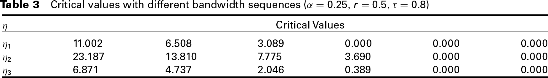
Table 1 shows the critical values with several choices of $α$ and $r$ with $τ = 0.2$ and $m = 5 000$ Monte Carlo samples, and a bandwidth sequence $(5, 7, 10, 13, 17, 21, 24, 28, 36, 45) / 365$ scaled to the interval $[0, 1]$ . Critical values decrease when $α$ increases, and increase when $r$ increases.

Table 1:

Critical values with different $α$ and $r$ ( $τ = 0.2$ )

$τ$	Critical Values
0.05	10.357	7.605	4.888	1.248	0.000	0.000
0.25	15.782	11.332	8.440	4.354	0.908	0.000
0.50	21.714	15.427	10.351	3.594	0.000	0.000
0.75	15.283	10.932	8.396	3.949	0.840	0.000
0.95	10.789	7.686	4.943	1.208	0.000	0.000

Table 2 shows the critical values for different $τ$ s with $α = 0.25, r = 0.5$ and $m = 5 000$ Monte Carlo samples, and a bandwidth sequence $(5, 7, 10, 13, 17, 21, 24, 28, 36, 45) / 365$ scaled to the interval $[0, 1]$ . Critical values behave similarly for symmetric $τ$ .

Table 2:

Critical values with different $τ$ ( $α = 0.25, r = 0.5$ )

$α$	$r$	Critical Values
0.25	0.5	16.971	11.539	8.133	3.584	0.044	0.000
0.25	0.75	20.218	13.743	9.336	3.131	0.000	0.000
0.25	1	24.676	16.270	9.308	4.214	1.561	0.000
0.5	0.5	12.823	9.619	7.205	3.703	0.949	0.000
0.75	0.5	11.249	7.222	4.244	0.181	0.000	0.000

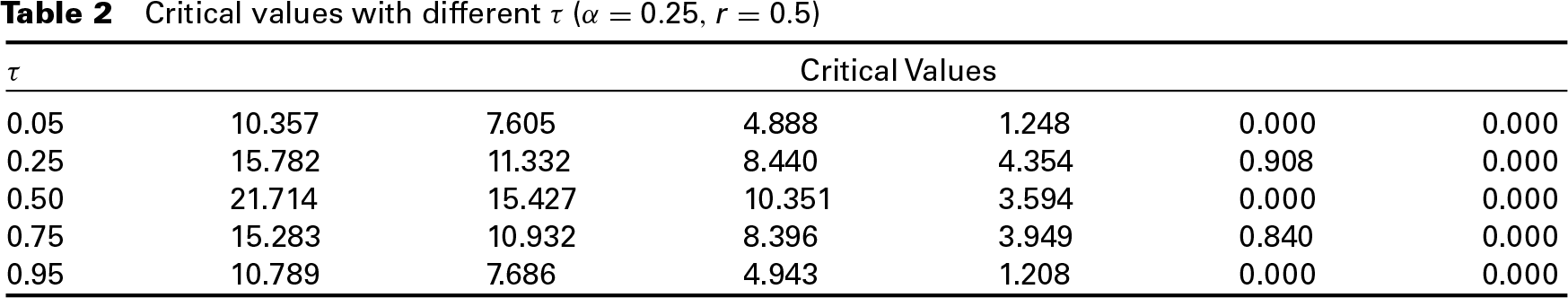
Table 3 shows the critical values for the following alternative bandwidth sequences, with $α = 0.25, r = 0.5, τ = 0.8$ and $m = 5 000$ Monte Carlo samples.

\begin{matrix} η_{1} & = (5, 7, 10, 13, 17, 21, 24, 28, 36, 45) / 365 \\ η_{2} & = (10, 13, 17, 21, 24, 28, 36, 45, 49, 60) / 365 \\ η_{3} & = (2, 3, 5, 7, 10, 13, 17, 21, 24, 28) / 365 \end{matrix}

Although the critical values differ for different bandwidth sequences, they indicate the same patterns (finite and decreasing).

Table 3:

Critical values with different bandwidth sequences ( $α = 0.25, r = 0.5, τ = 0.8$ )

$η$	Critical Values
$η_{1}$	11.002	6.508	3.089	0.000	0.000	0.000
$η_{2}$	23.187	13.810	7.775	3.690	0.000	0.000
$η_{3}$	6.871	4.737	2.046	0.389	0.000	0.000

Overall, although the critical values differ for different bandwidth sequences, $α$ , $r$ and $τ$ , the same finite and decreasing patterns indicate that the adaptation algorithm can be completed in maximum $K = 6$ steps, as the values of critical values decrease to zero in 6 step.

5.2 Simulation 2

In this simulation study, we compare the performance of our proposed approach to SWH's method as well as two other bandwidth selection techniques. One proposal comes from (ng, 2007), in which they considered constrained quantile estimations using linear or quadratic splines (implemented with R function cobs in Package cobs), and the other is from (Yu, 1998), in which they considered a rule of thumb bandwidth (implemented with R function lprq in Package quantreg).

We generate one training data of size 2 000 and 500 test datasets of size 500 from the model

Y = m (X) + σ (X) ε,

(5.1)

where the univariate input $X$ follows a uniform distribution on $[4, 4]$ and $m (X)$ is a non-linear function of $X$

m (X) = (1 - X + 2 X^{2}) e^{- 0.5 x^{2}},

and the scale factor $σ (X)$ is linearly increasing in $X$ with the form

σ (X) = \frac{1}{5} (1 + 0.2 x) .

Therefore, Equation (5.1) is a heteroskedastic model.

In this simulation, we consider three different types of random errors for $ε$ : $N (0, 1)$ , $t (3)$ and $χ^{2} (3)$ , respectively. Therefore, the true $τ$ -th conditional quantile function of $Y$ given $X = x$ can be expressed as

Q_{Y} (τ | x) = m (x) + σ (x) F_{τ}^{- 1} (ε),

where $F_{τ}^{- 1} (ε)$ is the $τ$ -th quantile of $ε$ . Figure 3 presents the training data generated under this scenario with their true $τ$ -th conditional quantile functions $Q_{Y} (τ | x), τ \in c (0.05, 0.50, 0.95)$ . Note that the non-linear function $m (X)$ in the right figure is not identical to the true conditional median function $Q_{Y} (0.50 | x)$ as the random error $χ^{2} (3)$ is an asymmetric distribution.

Figure 3:

Simulated training data and true conditional quantile functions with $τ \in c (0.05, 0.50, 0.95)$

We aim to compare the prediction power of the aforementioned four methods for the prediction of the conditional quantile function by 500 test datasets, in terms of three measurements, namely, the root mean square error (RMSE), the mean absolute errors (MAE) and the Theil-U statistic, which is a relative accuracy measure that compares the forecast results with the nave forecast (Theil, 1966):

\begin{matrix} RMSE (τ) & = \sqrt{\frac{1}{n} \sum_{i = 1}^{n} {(Q_{Y_{i}} (τ | x) - {\hat{Q}}_{Y_{i}} (τ | x))}^{2}}, \\ MAE (τ) & = \frac{1}{n} \sum_{i = 1}^{n} |Q_{Y_{i}} (τ | x) - {\hat{Q}}_{Y_{i}} (τ | x)|, \\ TheiU (τ) & = \sqrt{\frac{\sum_{i = 2}^{n} {(\frac{{\hat{Q}}_{Y_{i}} (τ | x) - Q_{Y_{i}} (τ | x)}{Q_{Y_{i - 1}} (τ | x)})}^{2}}{\sum_{i = 2}^{n} {(\frac{Q_{Y_{i}} (τ | x) - Q_{Y_{i - 1}} (τ | x)}{Q_{Y_{i - 1}} (τ | x)})}^{2}}}, \end{matrix}

where ${\hat{Q}}_{Y_{i}} (τ | x)$ is the prediction of the true conditional quantile $Q_{Y_{i}} (τ | x)$ . The smaller the measurement value is, the better the method is. The three measurements are implemented with R function av.res in package AnalyzeTS.

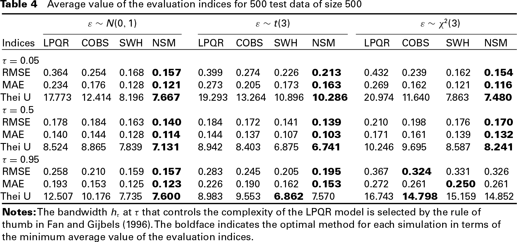
The superiority of the proposed NSM approach is demonstrated in Table 4 which summarizes the results for three values of $τ$ s: 0.05, 0.50 and 0.95, based on the 500 replications. Note that Simulation 2 is implemented with critical values $η =$ (5,7,10,13,17,21,24,28,36,45)/365, simulated from $ALD (0, 1, τ)$ (coincide with the likelihood) with $α = 0.25$ , $r = 0.5$ . The bold face values show that both SWH's method and the proposed NSM approach are superior to LPQR and COBS, while the proposed approach performs slightly better than SWH. It is encouraging to see that the proposed approach approximates well under Gaussian error and also provides excellent results under the circumstance of heavy tail and asymmetric distributions, such as $t (3)$ and $χ^{2} (3)$ .

Table 4:

Average value of the evaluation indices for 500 test data of size 500

	$ε \sim N (0, 1)$				$ε \sim t (3)$				$ε \sim χ^{2} (3)$
Indices	LPQR	COBS	SWH	NSM	LPQR	COBS	SWH	NSM	LPQR	COBS	SWH	NSM
$τ = 0.05$
RMSE	0.364	0.254	0.168	0.157	0.399	0.274	0.226	0.213	0.432	0.239	0.162	0.154
MAE	0.234	0.176	0.128	0.121	0.273	0.205	0.173	0.163	0.269	0.162	0.121	0.116
Thei U	17.773	12.414	8.196	7.667	19.293	13.264	10.896	10.286	20.974	11.640	7.863	7.480
$τ = 0.5$
RMSE	0.178	0.184	0.163	0.140	0.184	0.172	0.141	0.139	0.210	0.198	0.176	0.170
MAE	0.140	0.144	0.128	0.114	0.144	0.137	0.107	0.103	0.171	0.161	0.139	0.132
Thei U	8.524	8.865	7.839	7.131	8.942	8.403	6.875	6.741	10.246	9.695	8.587	8.241
$τ = 0.95$
RMSE	0.258	0.210	0.159	0.157	0.283	0.245	0.205	0.195	0.367	0.324	0.331	0.326
MAE	0.193	0.153	0.125	0.123	0.226	0.190	0.162	0.153	0.272	0.261	0.250	0.261
Thei U	12.507	10.176	7.735	7.600	8.983	9.553	6.862	7.570	16.743	14.798	15.159	14.852

Notes: The bandwidth $h_{τ}$ at $τ$ that controls the complexity of the LPQR model is selected by the rule of thumb in (fan, 1996). The boldface indicates the optimal method for each simulation in terms of the minimum average value of the evaluation indices.

5.3 Real-world data application

In this section, we demonstrate the efficacy of our the proposed alternative approach with one benchmark example that comes from the second and third health examination surveys of the United States (National Center for Health Statistics, 1970, 1973). Taken together these provide data on the anthropometry of children between the ages of 6 years and under 18 years, with from 400 to 600 children of each sex seen in each year of age (cole, 1988). Here, along with (Yu, 1998), the weights and ages of 4 011 US girls were analysed.

The scatter plot in Figure 4a displays weight against age for a sample of 4 011 US girls, where age is a univariate regressor $X \in R^{1}$ for simplicity. It is evident that the distribution is left skewed and presents long tails, suggesting that focusing on the centre is not sufficient for a comprehensive description of a weight distribution. Such observation motivates the use of quantile regression, where a complete picture of weight distribution is captured by conditional quantiles.

We then continue by inspecting the relation between weight and age in the sample. In Figure 4, we display the bandwidth sequence (upper right panels), boxplot of adapted bandwidth (lower right panels) showing the relationship between the adapted estimator and the bandwidth index, and smoothed quantile curves for quantile 99% (4b) and 1% (4a), respectively, by using the alternative NSM likelihood function. Both adaptations show that the proposed bandwidth selection is well adapted over the data distribution, which provides smooth fitting and better adaptation when $τ$ tends to extreme quantiles. Furthermore, Figure 5 shows that the non-quantile crossing property holds for the rule in Section 4.2, which is based on the alternative normal scale-mixture likelihood function.

Figure 4:

Smoothed quantile curves (in red) for US Health Examination Surveys with $τ = 0.01$ and $τ = 0.99$ via alternative normal scale-mixture likelihood (left panel). The bandwidth sequence (upper right); boxplot of adaptive bandwidth (lower right)

Figure 5:

Smoothed quantile curves for US Health Examination Surveys with $τ = c (0.05, 0.25, 0.5, 0.75, 0.95)$ via alternative normal scale-mixture likelihood function

6 Discussions and concluding remarks

The kernel-weighted likelihood function Equation (2.5) in SWH's paper is a local ALD-based likelihood function. The ALD-based inference has nowadays become a powerful tool for formulating different quantile regression techniques, particularly for the development of different Bayesian inference techniques for quantile regression. The ALD-based inference for non-Bayesian methods includes (taylor, 2016) in financial risk analysis and (geraci, 2007) in longitudinal data analysis and among others. The local ALD-based likelihood approach in the paper uses an alternative ALD-type of likelihood. The resulting automatic bandwidth selection rule not only enjoys the PCs of SWH (which postulates that the risk is smaller than the upper bound for the risk of the estimator ${\tilde{θ}}_{k} (x)$ ) but also guarantees non-quantile curve crossing. Theoretical results also claim that the proposed adaptive procedure performs well, which would minimize the local estimation risk for the problem at hand. We illustrate the performance of the procedure by comparing the Lidar dataset with SWH's approach and analysing an extended real data application. In particular, we show that the performance of the adaptive procedure is promising in practice, especially for smoothing extreme quantile curves.

Moreover, the proposed approach can also be extended to the $d$ -dimensional case $X \in 𝕣^{d}$ with $d > 1$ , under the non-parametric additive modelling framework (yu, 2004). That is, let $Y$ be a real-valued dependent variable and $X = (X^{(1)}, \dots, X^{(d)}) \in 𝕣^{d}$ is a vector of explanatory variables. Let $f (x)$ be a $d$ -dimensional $τ$ th quantile regression function of $Y$ given $X = x$ . Suppose that the $τ$ th quantile function $f (x)$ is modelled as an additive function of $(x^{(1)}, \dots, x^{(d)})$ ,

f (x) = \sum_{l = 1}^{d} f^{(l)} (x^{(l)}),

(6.1)

where each $f^{(l)} (x^{(l)})$ can be fitted by the proposed approach in Section 3 and the whole $f (x)$ can be further derived via backfitting algorithm used in (yu, 2004). For example, without of generality, consider a local linear regression with $p = 2$ , for $l = 1, \dots, d$ ,

({\hat{a}}^{(l)}, {\hat{b}}^{(l)}) = \underset{a, b}{argmin} \sum_{i = 1}^{n} ρ_{τ} (Y_{i} - a - b (X_{i}^{(l)} - x^{(l)})) (\frac{X_{i}^{(l)} - x^{(l)}}{h^{(l)}}),

where $K (\cdot)$ is a kernel function and $h^{(l)} (l = 1, \dots, d)$ is the bandwidth for estimating $f^{(l)} (x^{(l)})$ in the earlier setting.

Acknowledgements

We thank the editor, the associate editor and two anonymous reviewers for their constructive comments, which helped us to improve the manuscript.

Declaration of conflicting interests

The author(s) declared no potential conflicts of interest with respect to the research, authorship and/or publication of this article

Funding

The authors declared: The research was partially supported by Major Program of the National Natural Science Foundation of China (Grant No. 71490725) and the BUL Research Leave funding, the National Science Foundation of China (No 11261048).

Appendix

Recall: $w_{k} = diag (\frac{w_{1}^{(k)}}{δ^{2} z_{1}}, . . ., \frac{w_{n}^{(k)}}{δ^{2} z_{n}})$ .

Assumption Consider a finite sequence of scales $w_{k} = diag (w_{1}^{(k)}, \dots, w_{n}^{(k)})$ , where the $p \times n$ matrix $ψ^{T} w_{1}$ is of full row rank.

Assumption For any fixed $x$ and the method of localization with $w_{i}^{(k)} (x) \geq 0$ , the following relation holds:

w_{1} (x) \leq w_{2} (x) \leq \dots \leq w_{n} (x) .

Assumption Assume that the true regression model

Y_{i} = f_{0} (X_{i}) + μ_{0} z_{0, i} + δ_{0}^{2} \sqrt{z_{0, i}} e_{i},

considering the regression model (3.2), where $z_{0} = diag (δ_{0}^{2} z_{0, 1}, \dots, δ_{0}^{2} z_{0, n})$ stands for the unknown true covariance matrix, where $z_{0, i}$ is the true value of Equation (3.2), there exists $η \in [0, 1)$ such that

1 - η \leq \frac{δ_{0}^{2} z_{0, i}}{δ^{2} z_{i}} \leq 1 + η ​ ​ for ​ all ​ i = 1, \dots, n .

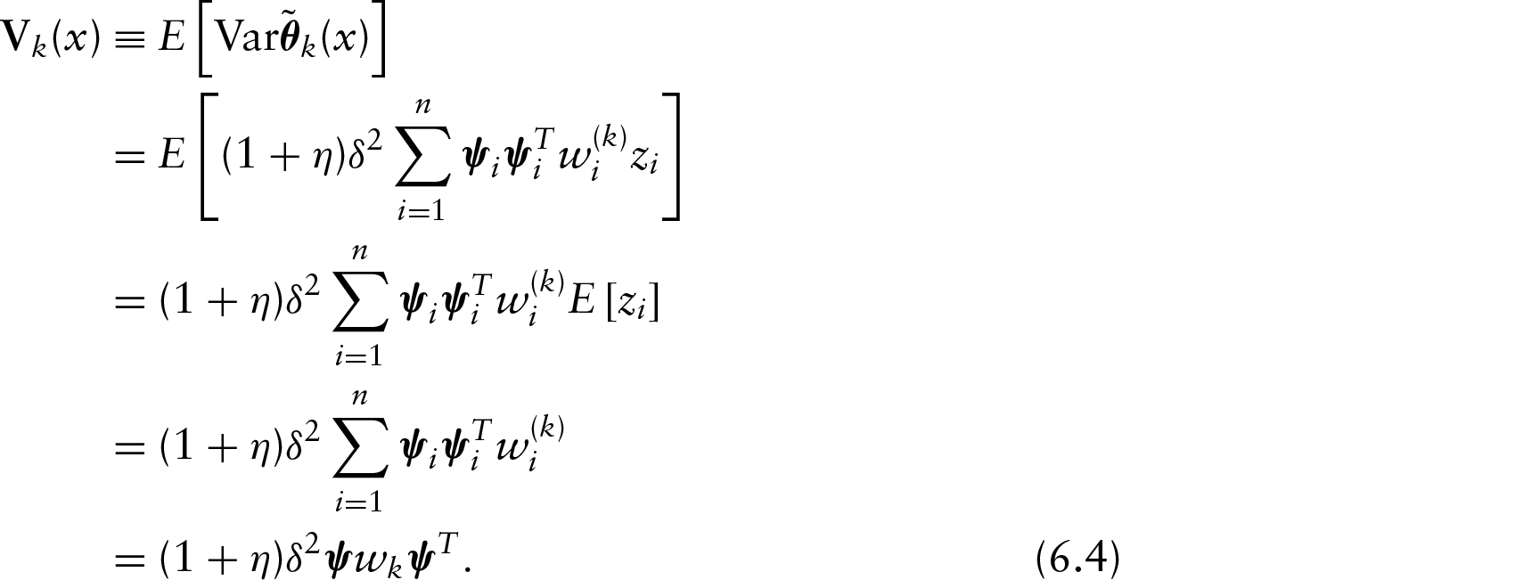
Assuming (A3), the true covariance matrix $z_{0} ⪯ z (1 + η)$ , and the conditional variance of the estimate ${\tilde{θ}}_{k} (x)$ is bounded with ${({ψ w}_{k} ψ^{T})}^{- 1}$ : as follows:

\begin{matrix} Var ({\tilde{θ}}_{k} (x)) & = & {({ψ w}_{k} ψ^{T})}^{- 1} {ψ w}_{k} z_{0} w_{k} ψ^{T} {({ψ w}_{k} ψ^{T})}^{- 1} \\ ⪯ & (1 + η) {({ψ w}_{k} ψ^{T})}^{- 1} {ψ w}_{k} {z w}_{k} ψ^{T} {({ψ w}_{k} ψ^{T})}^{- 1} \end{matrix}

\begin{matrix} = & (1 + η) {({ψ w}_{k} ψ^{T})}^{- 1} {ψ z}^{- 1 / 2} w_{k}^{2} z^{- 1 / 2} ψ^{T} {({ψ w}_{k} ψ^{T})}^{- 1} \\ ⪯ & (1 + η) {({ψ w}_{k} ψ^{T})}^{- 1} {ψ z}^{- 1 / 2} w_{k} z^{- 1 / 2} ψ^{T} {({ψ w}_{k} ψ^{T})}^{- 1} \\ = & (1 + η) {({ψ w}_{k} ψ^{T})}^{- 1} ({ψ w}_{k} ψ^{T}) {({ψ w}_{k} ψ^{T})}^{- 1} \\ = & (1 + η) {({ψ w}_{k} ψ^{T})}^{- 1} \\ = & (1 + η) {(\sum_{i = 1}^{n} ψ_{i} ψ_{i}^{T} \frac{w_{i}^{(k)}}{δ^{2} z_{i}})}^{- 1} . \end{matrix}

(6.2)

According to the basic property of quadratic equation, consider a simple example ${(\frac{1}{z_{1}} + \frac{1}{z_{2}})}^{- 1}$ and there always holds ${(\frac{1}{z_{1}} + \frac{1}{z_{2}})}^{- 1} = \frac{z_{1} z_{2}}{z_{1} + z_{2}} \leq z_{1} + z_{2}$ , with $z_{1}, z_{2} > 0$ . The same procedure may be easily adapted to Equation(6.2) as follows:

\begin{matrix} Var ({\tilde{θ}}_{k} (x)) & ⪯ & (1 + η) \sum_{i = 1}^{n} ψ_{i} ψ_{i}^{T} w_{i}^{(k)} δ^{2} z_{i} \\ = & (1 + η) δ^{2} \sum_{i = 1}^{n} ψ_{i} ψ_{i}^{T} w_{i}^{(k)} z_{i} . \end{matrix}

(6.3)

Therefore, the unconditional variance of the estimate ${\tilde{θ}}_{k} (x)$ as follows is bounded with $ψ w_{k} ψ^{T}$

\begin{matrix} V_{k} (x) & \equiv & E [Var {\tilde{θ}}_{k} (x)] \\ = & E [(1 + η) δ^{2} \sum_{i = 1}^{n} ψ_{i} ψ_{i}^{T} w_{i}^{(k)} z_{i}] \\ = & (1 + η) δ^{2} \sum_{i = 1}^{n} ψ_{i} ψ_{i}^{T} w_{i}^{(k)} E [z_{i}] \\ = & (1 + η) δ^{2} \sum_{i = 1}^{n} ψ_{i} ψ_{i}^{T} w_{i}^{(k)} \\ = & (1 + η) δ^{2} ψ w_{k} ψ^{T} . \end{matrix}

(6.4)

Proof of Theorem 1.

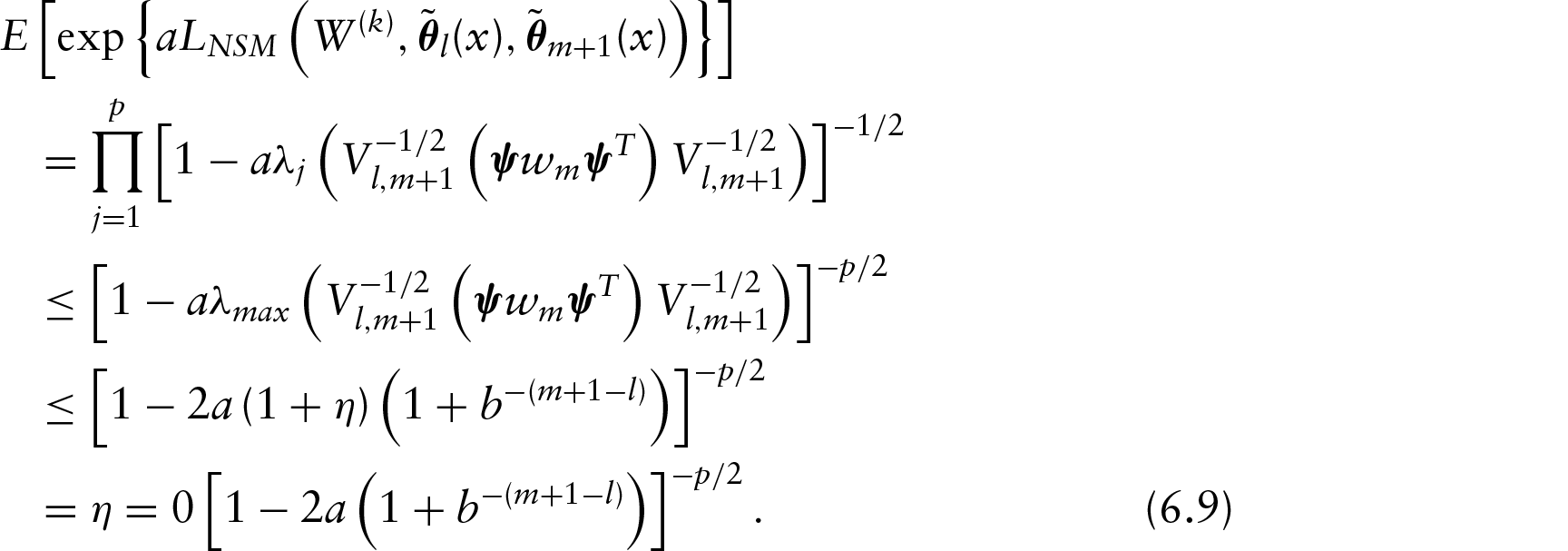
\begin{matrix} 𝔼 {|{({\tilde{θ}}_{k} (x) - {\hat{θ}}_{k} (x))}^{T} (ψ w_{k} (x) ψ^{T}) ({\tilde{θ}}_{k} (x) - {\hat{θ}}_{k} (x))|}^{r} \\ = & \sum_{m = 1}^{k - 1} 𝔼 {|{({\tilde{θ}}_{k} (x) - {\tilde{θ}}_{m} (x))}^{T} (ψ w_{k} ψ^{T}) ({\tilde{θ}}_{k} (x) - {\tilde{θ}}_{m} (x))|}^{r} I \{{\hat{θ}}_{k} (x) = {\tilde{θ}}_{m} (x)\} . \end{matrix}

(6.5)

The event $\{{\hat{θ}}_{k} (x) = {\tilde{θ}}_{m} (x)\}$ happens if for some $l = 1, \dots, m$ , $T_{l, m + 1} > ζ_{l}$ . Hence,

\{{\hat{θ}}_{k} (x) = {\tilde{θ}}_{m} (x)\} \subseteq ⋃_{l = 1}^{m} {T_{l, m + 1} > ζ_{l}} .

Further, combined with the Cauchy–Schwarz inequality, for any positive $a$ :

\begin{matrix} 𝔼 {|{({\tilde{θ}}_{k} (x) - {\tilde{θ}}_{m} (x))}^{T} (ψ w_{k} ψ^{T}) ({\tilde{θ}}_{k} (x) - {\tilde{θ}}_{m} (x))|}^{r} I \{{\hat{θ}}_{k} (x) = {\tilde{θ}}_{m} (x)\} \\ = 𝔼 {|2 L_{NSM} (W^{(k)}, {\tilde{θ}}_{k} (x), {\tilde{θ}}_{m} (x))|}^{r} I \{{\hat{θ}}_{k} (x) = {\tilde{θ}}_{m} (x)\} \\ \leq \sum_{l = 1}^{m} e^{- \frac{a}{4} ζ_{l}} {\{𝔼 [{|2 L_{NSM} (W^{(k)}, {\tilde{θ}}_{k} (x), {\tilde{θ}}_{m} (x))|}^{2 r}]\}}^{\frac{1}{2}} \\ {\{𝔼 [\exp \{{aL}_{NSM} (W^{(k)}, {\tilde{θ}}_{l} (x), {\tilde{θ}}_{m + 1} (x))\}]\}}^{\frac{1}{2}} . \end{matrix}

(6.6)

Among which,

\begin{matrix} E [{|2 L_{NSM} (W^{(k)}, {\tilde{θ}}_{k} (x), {\tilde{θ}}_{m} (x))|}^{2 r}] \\ = 2 r \int_{0}^{\infty} P \{2 L_{NSM} (W^{(k)}, {\tilde{θ}}_{k} (x), {\tilde{θ}}_{m} (x)) \geq ζ\} ζ^{2 r - 1} d ζ \\ \leq 2 r \int_{0}^{\infty} P \{γ \geq ζ {[2 (1 + η) (1 + b^{(k - m)})]}^{- 1}\} ζ^{2 r - 1} d ζ \\ = 2^{2 r} {(1 + η)}^{2 r} {(1 + b^{(k - m)})}^{2 r} E {|χ_{p}^{2}|}^{r} \end{matrix}

(6.7)

\begin{matrix} = η = 0 2^{2 r} C (p, 2 r) {(1 + b^{(k - m)})}^{2 r}, \end{matrix}

(6.8)

and

\begin{matrix} E [\exp \{{aL}_{NSM} (W^{(k)}, {\tilde{θ}}_{l} (x), {\tilde{θ}}_{m + 1} (x))\}] \\ = \prod_{j = 1}^{p} {[1 - a λ_{j} (V_{l, m + 1}^{- 1 / 2} (ψ w_{m} ψ^{T}) V_{l, m + 1}^{- 1 / 2})]}^{- 1 / 2} \\ \leq {[1 - a λ_{\max} (V_{l, m + 1}^{- 1 / 2} (ψ w_{m} ψ^{T}) V_{l, m + 1}^{- 1 / 2})]}^{- p / 2} \\ \leq {[1 - 2 a (1 + η) (1 + b^{- (m + 1 - l)})]}^{- p / 2} \\ = η = 0 {[1 - 2 a (1 + b^{- (m + 1 - l)})]}^{- p / 2} . \end{matrix}

(6.9)

Therefore, we obtain

\begin{matrix} E {|{({\tilde{θ}}_{k} (x) - {\hat{θ}}_{k} (x))}^{T} (ψ w_{k} (x) ψ^{T}) ({\tilde{θ}}_{k} (x) - {\hat{θ}}_{k} (x))|}^{r} \\ \leq 2^{r} \sqrt{C (p, 2 r)} (1 - 4 a)^{- p / 4} \sum_{m = 1}^{k - 1} \sum_{l = 1}^{m} e^{- \frac{μ}{4} ζ_{l}} {(1 + b^{k - m})}^{r} \\ \leq 2^{2 r} \sqrt{C (p, 2 r)} (1 - 4 a)^{- p / 4} (1 - b^{- r}) \sum_{l = 1}^{k - 1} e^{- \frac{μ}{4} ζ_{l}} b^{r (k - l)} . \end{matrix}

(6.10)

For any $l < k < K$ , with an arbitrary constant $μ \in (0, 1 / 4)$ , the choice of the threshold of the form

ζ_{l} = \frac{4}{μ} \{r (K - l) \log b + \log \frac{K}{α} - \frac{p}{4} \log (1 - 4 μ) - \log (1 - b^{- r}) + \overset{̅}{C} (p, r)\},

where $\overset{̅}{C} (p, r) = \log \{\frac{2^{2 r} {[Γ (2 r + p / 2) Γ (p / 2)]}^{1 / 2}}{Γ (r + p / 2)}\}$ provides the required PC bounds.

E {|{({\tilde{θ}}_{k} (x) - {\hat{θ}}_{k} (x))}^{T} (ψ w_{k} (x) ψ^{T}) ({\tilde{θ}}_{k} (x) - {\hat{θ}}_{k} (x))|}^{r} \leq α C (p, r), ​ for ​ all ​ k = 2, \dots, K .

References

Akaike

(1973) Information theory and an extension of the maximum likelihood principle. In Second International Sympo- sium on Information Theory , edited by PETROV

B. N.

CSAKI

pages 267–281. Budapest: Akademiai Kiado.

Bondell

Reich

Wang

(2010) Noncros- sing quantile regression curve estimation. Biometrika , 97, 825–838.

Cai

(2008) Nonparametric quantile estimations for dynamic smooth coefficient models. Journal of the American Statistical Association , 103, 1595–1608.

Chaudhuri

(1991) B Nonparametric estimates of regression quantiles and their local Bahadur representation. The Annals of Statistics , 19, 760–777.

Cole

(1988) Fitting smoothed centile curves to reference data. Journal of the Royal Statistical Society, Series A (Statistics in Society) , 151, 385–418.

Craven

Wahba

(1979) Smoothing noisy data with spline functions: Estimating the correct degree of smoothing by the method of generalized cross-validation. Numerical Mathematics , 31, 377–403.

Dabo-Niang

Laksaci

(2012) Nonpara- metric quantile regression estimation for functional dependent data. Numerical Mathematics , 41, 1254–1268.

Dette

Volgushev

(2008) Non-crossing non-parametric estimates of quantile curves. Journal of the Royal Statistical Society: Series B (Statistical Methodology) , 70, 609–627.

Fan

Gijbels

(1996) Local Polynomial Mod- elling and Its Applications: Monographs on Statistics and Applied Probability 66 . CRC Press.

10.

Geraci

Bottai

(2007) Quantile regres- sion for longitudinal data using the asymmetric Laplace distribution. Biosta- tistics , 8, 140–154.

11.

Hall

, Wol

Yao

(1999) Methods for estimating a conditional distribution function. Journal of the American Statistical Association , 94, 154–163.

12.

Hardle

Mammen

(1993) Comparing nonparametric versus parametric regression fits. The Annals of Statistics , 21, 1926–47.

13.

(1997) Quantile curves without crossing. The American Statistician , 51, 186–192.

14.

Hurvich

, Simono

Tsai

(1998) Smoo- thing parameter selection in nonparametric regression using an improved Akaike information criterion. Journal of the Royal Statistical Society: Series B (Statistical Methodology) , 60, 271–293.

15.

Jones

(2007) Improve double kernel local linear quantile regression. Statistical Modelling , 7, 377–389.

16.

Koenker

(2005) Quantile Regression . New York, NY: Cambridge University Press.

17.

Kong

Xia

(2017) Uniform Bahadur representation for nonparametric censored quantile regression: A redistribution-of- mass approach. Econometric Theory , 33, >242–261.

18.

Kozumi

Kobayashi

(2011) Gibbs sampling methods for Bayesian quantile regression. Journal of Statistical Compu- tation and Simulation , 81, 1565–1578.

19.

Liu

(2011) Simultaneous multiple non-crossing quantile regression estimation using kernel constraints. Journal of Nonparametric Statistics , 23, 415–437.

20.

Muggeo

Sciandra

Tomasello

Calvo

(2013) Estimating growth charts via nonparametric quantile regression: A practical framework with application in ecology. Environmental and Ecological Statistics , 20, 519–531.

21.

Maechler

(2007) A fast and efficient implementation of qualitatively constrained quantile smoothing splines. Statistical Modelling , 7, 315–328.

22.

Yoon

(2015) Nonparametric estimation and inference on conditional quantile processes. Journal of Econome- trics , 185, 1–19.

23.

Reed

(2010) Efficient Gibbs sampling for Bayesian quantile regression (Technical report). London: Brunel University London.

24.

Ruppert

Sheather

Wand

(1995) An effective bandwidth selector for local least squares regression. Journal of the American Statistical Association , 90, 1257–1270.

25.

Schaumburg

(2012) Predicting extreme value at risk: Nonparametric quantile regression with refinements from extreme value theory. Computational Statistics & Data Analysis , 56, 4081–4096.

26.

Serdyukova

(2012) Spatial adaptation in heteroscedastic regression: Propagation approach. Electronic Journal of Statistics , 6, 861–907.

27.

Spokoiny

Vial

(2009) Parameter tuning in pointwise adaptation using a propagation approach. The Annals of Statistics , 37, 2783–2807.

28.

Spokoiny

Wang

Härdle

(2013) Local quantile regression. Journal of Statis- tical Planning and Inference , 143, 1109–1129.

29.

Takezawa

(2005) Introduction to Nonpara- metric Regression . Vol. 606. John Wiley & Sons.

30.

Taylor

(2016) Using auto-regressive logit models to forecast the exceedance probability for financial risk management. Journal of the Royal Statistical Society: Series A (Statistics in Society) , 79, 1069– 1092.

31.

Theil

(1966) Applied Economic Forecasting . Amsterdam: North-Holland.

32.

Wand

Jones

(1995) Kernel Smoothing . London: Chapman & Hall.

33.

Jones

(1998) Local linear quantile regression. Journal of the American Statistical Association , 93, 228–237.

34.

(2004) Local linear additive quantile regression. Scandinavian Journal of Statistics , 31, 333–346.

Improved local quantile regression

Abstract

Keywords

Introduction

Kernel-weighted likelihood for local quantile regression

Figure 1:

The bandwidth sequences (upper panels) and smoothed quantile curves (lower panels) for the Lidar dataset using SWH's kernel-weighted likelihood

4.1 Adaptive bandwidth selection

The bandwidth sequences (upper panels) and smoothed quantile curves (lower panels) for the Lidar dataset using the alternative normal scale-mixture likelihood

5.1 Simulation 1

Table 1:

Critical values with different α and r ( τ = 0.2 )

Critical values with different τ ( α = 0.25 , r = 0.5 )

Critical values with different bandwidth sequences ( α = 0.25 , r = 0.5 , τ = 0.8 )

Simulated training data and true conditional quantile functions with τ ∈ c ( 0.05 , 0.50 , 0.95 )

Average value of the evaluation indices for 500 test data of size 500

Figure 4:

Smoothed quantile curves (in red) for US Health Examination Surveys with τ = 0.01 and τ = 0.99 via alternative normal scale-mixture likelihood (left panel). The bandwidth sequence (upper right); boxplot of adaptive bandwidth (lower right)

Smoothed quantile curves for US Health Examination Surveys with τ = c ( 0.05 , 0.25 , 0.5 , 0.75 , 0.95 ) via alternative normal scale-mixture likelihood function

Acknowledgements

Declaration of conflicting interests

Funding

Appendix

References

Critical values with different $α$ and $r$ ( $τ = 0.2$ )

Critical values with different $τ$ ( $α = 0.25, r = 0.5$ )

Critical values with different bandwidth sequences ( $α = 0.25, r = 0.5, τ = 0.8$ )

Simulated training data and true conditional quantile functions with $τ \in c (0.05, 0.50, 0.95)$

Smoothed quantile curves (in red) for US Health Examination Surveys with $τ = 0.01$ and $τ = 0.99$ via alternative normal scale-mixture likelihood (left panel). The bandwidth sequence (upper right); boxplot of adaptive bandwidth (lower right)

Smoothed quantile curves for US Health Examination Surveys with $τ = c (0.05, 0.25, 0.5, 0.75, 0.95)$ via alternative normal scale-mixture likelihood function