A clustering Bayesian approach for multivariate non-ordered circular data

1 Introduction

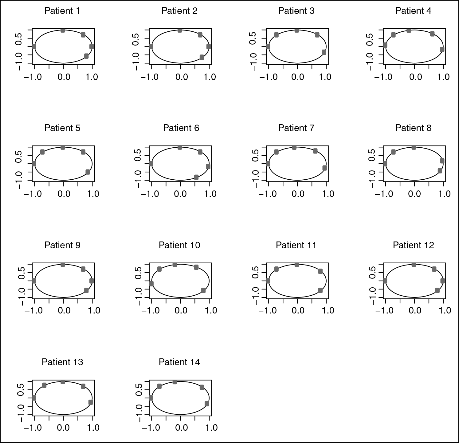
Circular and directional data arise in a number of different fields such as oceanography (wave direction), meteorology (wind direction) and biology (animal movement direction). The present article is motivated by circular data in medicine. Nowadays, intensity modulated radiation therapy (IMRT) has demonstrated its effectiveness for cancer treatment. The latest generation of radiotherapy machines projects multiple rays. Multiplying beams allows to concentrate radiation on the tumour while avoiding the massive irradiation of healthy areas. However, the selection of the incident angles of the treatment beams may be a crucial component of IMRT planning. Due to variations in tumour locations, size and patient anatomy, repositioning for the multiple beams takes a long time and is based on the planner's experience to find an optimal set of beams. So, establishing a small set of standardized beam bouquets for planning could be of valuable help. The set of beam bouquets could be determined by learning the beam configuration features from previous IMRT datasets. The multiple beams are fixed on a circle in the transverse plane around the patient. Consequently, an observation is composed of the k beams of a patient, that is, k circular measurements. A real dataset from post-operative treatment of liver cancer at the Institute of Sainte Catherine in Avignon, France, is represented in Figure 1. One actual observation consists of a (non-ordered) set of k angles rather than of a vector (ordered) of length k but to cope with the technical difficulty of dealing with sets, it is convenient to store the angles of each patient in a vector in increasing order (or in any other given order). Of course, the derived vectors may be very different even for similar sets of angles. This is easily seen by considering a simple case of two patients with angles { 1 ∘ , 60 ∘ , 100 ∘ , 150 ∘ , 180 ∘ } and { 60 ∘ , 100 ∘ , 150 ∘ , 180 ∘ , 359 ∘ } : the two patients should share the same cluster as the sets of angles are very similar (modulo 360), although the derived vectors are very different and, if any classical clustering method was applied, are not likely to share the same cluster.

OPEN IN VIEWER

Figure 1:

Real dataset of 14 patients with k = 5 angles. A point on the circle represents the location of a treatment beam

Abraham et al. (2013) proposed a first tool to assist the selection of beam orientations to enhance the therapist's experience. A suitable distance on the circle was defined and, for a fixed number of clusters, an algorithm based on simulated annealing was proposed. Yuan et al. (2015) generalized the precedent approach using k -medoids to cluster beam configuration features with different numbers of beams. These methods suffer from some major flaws. First, the number of clusters has to be supplied by the user. An additional procedure of model selection (AIC, BIC, RIC, silhouette index, … ) can be used to select the number of clusters, but an appropriate methodology that automatically finds this number would be very useful. Second, the final result is only one unique clustering, whereas there are probably other clusterings that could be acceptable. A final result with all possible clusterings and a probability of appearance for each could be of great help for the practitioner. These problems can naturally be solved with a Bayesian clustering method based on Dirichlet Process as it does not require a preselected number of clusters and provides different clusterings (possibly with different numbers of clusters) with their posterior probabilities. Also note that the Bayesian framework is well adapted to our application as the sample size is low and can be compensated to some extent by prior information.

Circular data have first been studied using classical non-Bayesian approaches. Three main models for circular data can be found in the litterature: the von-Mises distributions, the wrapped distributions and the projected normal distributions. The von-Mises distributions, first introduced by Von Mises (1918) and extended by Singh et al. (2002) and Mardia et al. (2008), are the natural analogues of the normal distribution on the sphere. The wrapped distributions (Mardia and Jupp, 2009) are based on a simple fact that a probability distribution on a circle can be obtained by wrapping a probability distribution defined on the real line. Projected normal distributions are obtained by projecting multivariate normal random variables radially onto the sphere (Presnell et al., 1998). These latter distributions allow for asymmetric and possible bimodal models. We refer the reader to Mardia and Jupp (2009) for a complete review on probability distributions of circular data.

Bayesian literature on circular data is more recent. Von Mises distributions are used in the univariate case in Damien and Walker (1999) and are applied to a change-point problem in SenGupta and Laha (2008). Wrapped distributions appear in Ravidran and Ghosh (2011), with a data augmentation algorithm to overcome some computational difficulties, and in Jona-Lasinio et al. (2012), to handle structured dependences between spatial measurements. Nuñez-Antonio and Gutiérrez-Peña(2005), Wang and Gelfand (2013) adapted the projected normal distributions in a Bayesian framework. A more sophisticated model was considered in Wang and Gelfand (2014) to capture structured spatial dependence for modelling directional data at different spatial locations. This model was then upgraded to capture joint structured spatial and temporal dependence (Wang et al., 2015). Then, it was extented to the important spherical case and to any dimension (Hernandez-Stumpfhauser et al., 2017). Also, it was adapted to a multidimensional time series forecasting framework coupled with a Dirichlet process by Mastrantonio et al. (2018).

Note that, for all the models cited earlier, each observation is simply a point on a circle or on a sphere while in our case, a single observation is made up of k ( k ≥ 2 ) non-ordered points on the circle. For this reason, these models cannot straightforwardly be adapted to our dataset. We propose an extension of the projected normal distribution to our data. This extension does not reduce to a simple projection of a multivariate normal distribution but enables us to model the multivariate and the non-ordered features of our data. We also provide an informative prior distribution on the relative locations of the k angles on the circle. This prior distribution expresses that the k angles are a priori regularly spaced on the circle. A new parameter is also introduced to control the variability of the angles on the circle. Inference on the variabiliy of the angles is of particular interest for a clustering purpose as an inadequate value of this parameter can alter the final results. The projected normal distribution is then associated with a Dirichlet process to perform clustering. Therefore, the proposed method includes an automated selection for the number of clusters.

In the present article, the Bayesian model is described in the next section. Section 3 is devoted to the inference of the parameters of the model. Section 4 provides a theoretical study to highlight the adaptability of our model to the multivariate and the non-ordered features of the data. Sections 5 and 6 provide empirical results first on simulated data and then on the real dataset that motivated the present work. A short conclusion is given in Section 7.

A simple way of generating distributions on the p -dimensional unit sphere S p is to radially project probability distributions originally defined on the p -dimensional space ℝ p (Presnell et al., 1998).. Let x be a random p -dimensional vector, then x / | | x | | is a random point on S p . If x has a p -variate normal distribution N p ( μ , Σ ) , then x / | | x | | is said to have a projected normal distribution, denoted by PN p ( μ , Σ ) . The literature has been first confined to the special case where p = 2 and Σ = I (Presnell et al., 1998; Nuñez-Antonio and Gutiérrez-Peña, 2005; Nuñez-Antonio et al., 2011). Then, Wang and Gelfand (2013) studied the projected normal family with a general covariance matrix Σ and refer to this richer class PN p ( μ , Σ ) as the general projected normal distribution. This general version allows asymmetry and bimodality (see Figure 2 in Wang and Gelfand, 2014). The general projected normal distribution is not identifiable because x / | | x | | is invariant to scale transformation. To overcome this problem, Wang and Gelfand (2013) fixed some variance parameters in Σ to provide identifiability.

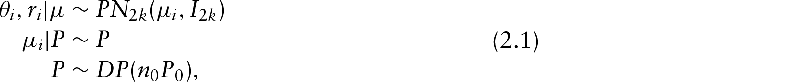
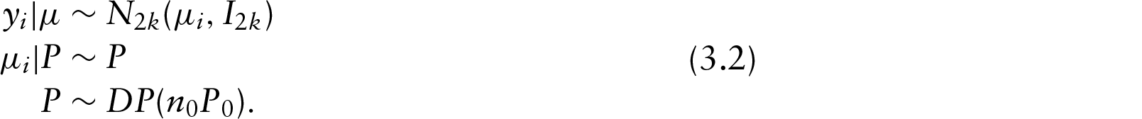
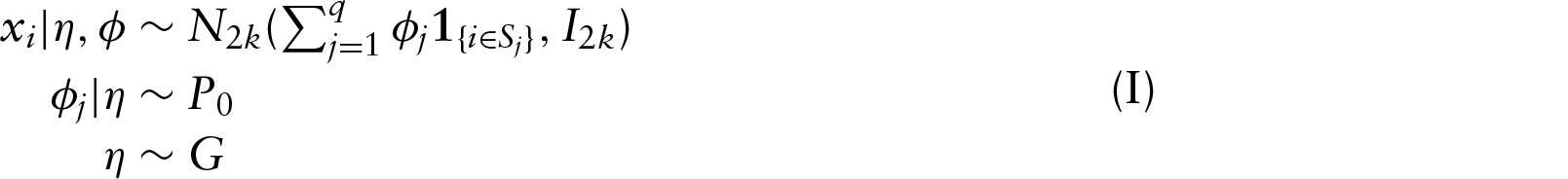
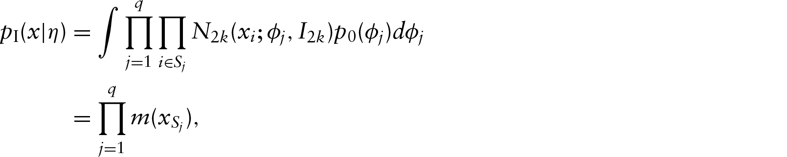
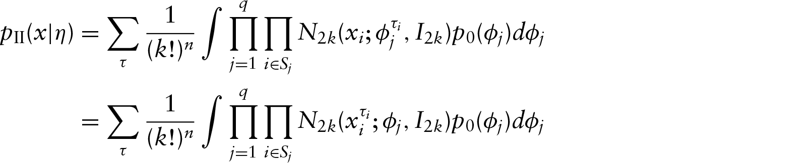
In a first step of simplification, we assume that the i th of the n observations is given by a vector of k angles θ i = ( θ i 1 , … , θ ik ) ′ ∈ [ 0 , 2 π [ k instead of a non-ordered set { θ i 1 , … , θ ik } . Using a projected normal distribution, we denote by x i = ( x i 1 , … , x ik ) ′ ∈ ( ℝ 2 ) k a random vector with distribution N 2 k ( μ i , I 2 k ) , where θ ij is defined as the radial projection of x ij on the unit circle of ℝ 2 . In other words, we have x ij = ( x ij 1 , x ij 2 ) ′ = ( r ij cos θ ij , r ij sin θ ij ) ′ for all i ∈ { 1 , … , n } and all j ∈ { 1 , … , k } where r ij denotes the Euclidean norm of x ij . Note that θ i is observed while r i = ( r i 1 , … , r ik ) ′ is not and is treated as an unknown parameter. We denote by PN 2 k ( μ i , I 2 k ) the joint distribution of ( θ i , r i ) . Clustering analysis will be based on a Dirichlet process mixture (DPM) model described as follows:

θ i , r i | μ ∼ PN 2 k ( μ i , I 2 k ) μ i | P ∼ P P ∼ DP ( n 0 P 0 ) ,

(2.1)

where μ = ( μ 1 , … , μ n ) and where DP ( n 0 P 0 ) denotes the Dirichlet process (DP) introduced by Ferguson (1973) with centre P 0 = N 2 k ( 0 , Σ 0 ) and precision parameter n 0 . The clustering properties of the DP are well known and date back to Blackwell and MacQueen (1973). It is shown that the parameter μ = ( μ 1 , … , μ n ) follows the Pólya urn scheme:

μ 1 ∼ P 0 μ i + 1 | μ 1 , … , μ i ∼ 1 n 0 + i ∑ j = 1 i δ μ i + n 0 n 0 + i P 0 , for i ≥ 2 ,

(2.2)

with δ μ i indicating the point measure on μ i . So, μ i + 1 may be equal to one of the previous μ i ’s or may be drawn from P 0 . This results in a positive probability of sharing the parameter value with previous observations; hence the clusters. In the sequel, we will denote by P & oacute ; lya ( n 0 P 0 ) the distribution of μ given by (2.2). Although the DPM is very popular for Bayesian clustering, other model-based cluster methods exist. For a review of these methods, we refer the reader to Quintana (2006); Lau and Green (2007); Fritsch and Ickstadt (2009) and references therein. Note that the DPM model does not require choosing the number of clusters. On the other hand, it is well known that the number of clusters can be controlled by n 0 . Learning about n 0 from the data may be addressed by assuming a Gamma prior distribution n 0 ∼ G ( a n 0 , b n 0 ) (Escobar and West, 1995).

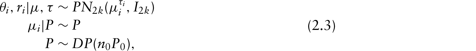
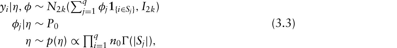
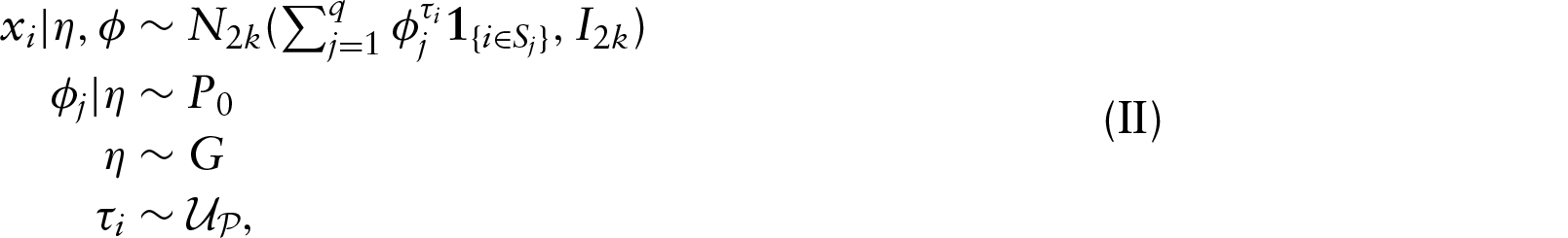
Now recall that the actual i th observation consists of a (non ordered) set of the form { θ i 1 , … , θ ik } rather than of a vector (ordered) θ i = ( θ i 1 , … , θ ik ) ′ . The impact of this simplification is quite easy to understand. Using model (2.1), two observations i 1 and i 2 with the same angles but in different orders would have a very low posterior probability of sharing the same cluster, that is μ i 1 = μ i 2 . We treat the observations as vectors for convenience, but we have to introduce a permutation parameter τ i to compensate this simplification. More precisely, for all μ i = ( μ i 1 ′ , … , μ ik ′ ) ′ and all permutation τ i of { 1 , … , k } , we set μ i τ i = ( μ i τ i ( 1 ) ′ , … , μ i τ i ( k ) ′ ) ′ ; μ i τ i can be viewed as a random permutation of the coordinates of μ i . Therefore, the clustering model becomes:

θ i , r i | μ , τ ∼ PN 2 k ( μ i τ i , I 2 k ) μ i | P ∼ P P ∼ DP ( n 0 P 0 ) ,

(2.3)

where τ = ( τ 1 , … , τ n ) and μ = ( μ 1 , … , μ n ) . The permutations τ i are assumed to be a priori independent with a uniform distribution U_P on the set P of permutations of { 1 , … , k } . The posterior probability that two observations i 1 and i 2 with the same angles but in different orders would share the same cluster is increased with model (2.3) as there exist some values of τ i 1 and τ i 2 such that μ i 1 τ i 1 = μ i 2 τ i 2 . A theoretical study of the impact of the symmetry introduced by τ i is given in Section 4.

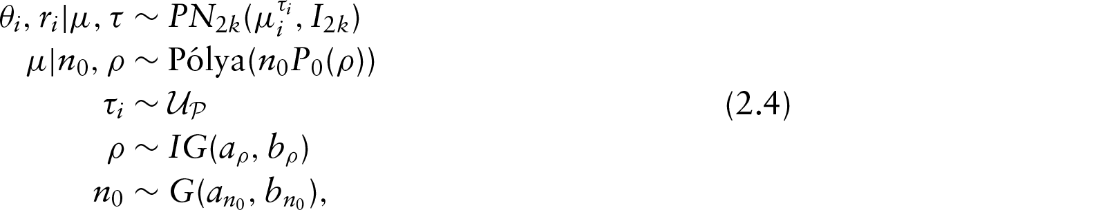
Prior information It is natural to assume that the k angles θ i 1 , … , θ ik are a priori distributed so that the radial projections x i 1 / ∥ x i 1 ∥ , … , x ik / ∥ x ik ∥ are roughly equally spaced on the unit circle. As x ij / ∥ x ij ∥ can be seen as a random change of μ ij / ∥ μ ij ∥ , this prior information can be incorporated into the covariance matrix Σ 0 of P 0 as follows. From (2.3), it is well known that the marginal distribution of μ i is P 0 = N 2 k ( 0 , Σ 0 ) . Denote by R the 2 × 2 -matrix of the rotation in ℝ 2 with angle 2 π / k and centre 0 and by ε ij , j ∈ { 2 , … , k } , k − 1 random variables with distribution ε ij ∼ N 2 ( 0 , I 2 ) . Assume that μ i 1 , ε i 2 , , … , ε ik are independent and set μ i 1 ∼ N 2 ( 0 , ρ I 2 ) where ρ is a positive number and μ ij = R j − 1 μ i 1 + ε ij for j ∈ { 2 , … , k } . It is important to note the influence of ρ on the distribution of μ i . First, it is shown in the Appendix that the expected value of ∥ μ ij ∥ is ρ π / 2 for j = 1 and ( ρ + 1 ) π / 2 for j ≥ 2 and that the components μ ij become more correlated and equally spaced as ρ increases. Furthermore, if we denote by v ij = μ ij / ∥ μ ij ∥ the radial projection of μ ij onto the unit circle, it is shown that ( v i 1 , … , v ik ) tends to ( v i 1 , Rv i 1 , … , R k − 1 v i 1 ) almost surely as ρ → ∞ and tends to ( ε i 1 / ∥ ε i 1 ∥ , … , ε ik / ∥ ε ik ∥ ) almost surely as ρ → 0 where ε i 1 , … , ε ik are independent and identically distributed random variables with distribution N 2 ( 0 , I 2 ) . In other words, the radial projections of the components of μ i are highly correlated and equally spaced for large values of ρ but approximately independent and uniformly distributed for small ones. The influence of ρ is also studied through some simulations in the sequel (see Subsection 5.1 and Figure 2).

Inference on ρ can be performed using an inverse gamma prior ρ ∼ IG ( a ρ , b ρ ) for which the full posterior conditional distribution will be calculated in the following section.

It is worth pointing out that the weak dissymmetry introduced in the definition of P 0 between μ i 1 and the other components of μ i leads to a convenient closed-form expression of Σ 0 from which closed-form expressions of the inverse Σ 0 − 1 and the determinant | Σ 0 | can be obtained as well. Such closed-form expressions and the full posterior conditional distribution of ρ could not have been obtained so easily with a perfect symmetric distribution P 0 . The calculations of Σ 0 , Σ 0 − 1 and | Σ 0 | are given in the Appendix. To highlight the dependence on ρ , Σ 0 will be also denoted by Σ 0 ( ρ ) in the sequel.

Finally, the complete Bayesian model can be expressed as follows:

θ i , r i | μ , τ ∼ PN 2 k ( μ i τ i , I 2 k ) μ | n 0 , ρ ∼ P oacute ; lya ( n 0 P 0 ( ρ ) ) τ i ∼ U P ρ ∼ IG ( a ρ , b ρ ) n 0 ∼ G ( a n 0 , b n 0 ) ,

(2.4)

where P 0 ( ρ ) = N 2 k ( 0 , Σ 0 ( ρ ) ) . By convention, it is assumed that the random variables at a stage of the hierarchy are independent.

We set θ = ( θ 1 , … , θ n ) , r = ( r 1 , … , r n ) , μ = ( μ 1 , … , μ n ) , τ = ( τ 1 , … , τ n ) and ξ = ( r , μ , τ , ρ , n 0 ) . Thus, the parameter is ξ and the observation is θ . We sample from the posterior distribution of ξ with a Metropolis–Hastings-within-Gibbs algorithm. In what follows, p stands for a generic notation for a density distribution.

agraph Simulations of μ We can restrict our attention to model (2.3) instead of the full model (2.4) for the simulations of μ as every component of ξ except μ remains fixed. An alternative parameter setting of μ , θ and ρ will prove useful. Denote x = ( x 1 , … , x n ) where x i = ( x i 1 ′ , … , x ik ′ ) ′ . First, note that the full conditional distribution of μ reduces to the conditional distribution of μ given ( x , n 0 , ρ , τ ) as there is a natural bijection between x ij and ( θ ij , r ij ) . Second, if we denote by N 2 k ( x i ; μ i , I 2 k ) the value of the density of N 2 k ( μ i , I 2 k ) at x i , it is easy to check that:

N 2 k ( x i ; μ i τ i , I 2 k ) = N 2 k ( x i τ i − 1 ; μ i , I 2 k ) ,

(3.1)

where τ i − 1 is the permutation such that x i τ i o τ i − 1 = x i . Consequently, if we set y i = x i τ i − 1 , sampling from the posterior distribution of μ in the DPM model (2.3) reduces to sampling from the posterior distribution of μ in the following conjugate DPM model:

y i | μ ∼ N 2 k ( μ i , I 2 k ) μ i | P ∼ P P ∼ DP ( n 0 P 0 ) .

(3.2)

There are several samplers for conjugate DPM models; for a review, we refer the reader to MacEachern (1998); Neal (2000); Griffin and Holmes (2010).Following the notations of Dahl (2003), we use a parameter setting of μ in terms of:

a set partition η = { S 1 , … , S q } for { 1 , … , n } where each S j represents a cluster, that is, μ i = μ j if there exists j 1 ∈ { 1 , … , q } such that i , j ∈ S j 1 and μ i ≠ μ j if there exist j 1 , i 1 ∈ { 1 , … , q } , i 1 ≠ j 1 such that i ∈ S i 1 , j ∈ S j 1 ,

y i | η , ϕ ∼ N 2 k ( ∑ j = 1 q ϕ j 1 { i ∈ S j } , I 2 k ) ϕ j | η ∼ P 0 η ∼ p ( η ) ∝ ∏ i = 1 q n 0 Γ ( | S j | ) ,

(3.3)

where | S j | is the cardinal of S j , 1 A is the indicator function for the event A , Γ denotes the gamma function and p stands for the generic notation for any density. We can integrate over the cluster location parameter ϕ analytically in (3.3) as P 0 is conjugate to the normal distribution of y i given η and ϕ . Then, we run the SAMS sampler of Dahl (2003) for simulating η . This sampler may improve the merge-split sampler initially proposed by Jain and Neal (2004). Once a simulation of η is obtained, it is easy to simulate the cluster location parameter ϕ from its full conditional which reduces to sample independently each ϕ j from a N 2 k ( Σ j ∑ i ∈ S j y i / | S j | , Σ j ) distribution with Σ j − 1 = | S j | − 1 I 2 k + Σ 0 − 1 ( ρ ) . As recommended by the previous authors, we combine three runs of the Metropolis–Hastings update of the SAMS sampler with a full scan of Gibbs sampling for μ (see MacEachern, 1994, for a presentation of this particular Gibbs sampler). Some details of the SAMS and the Gibbs samplers used in this article are given in the Appendix.

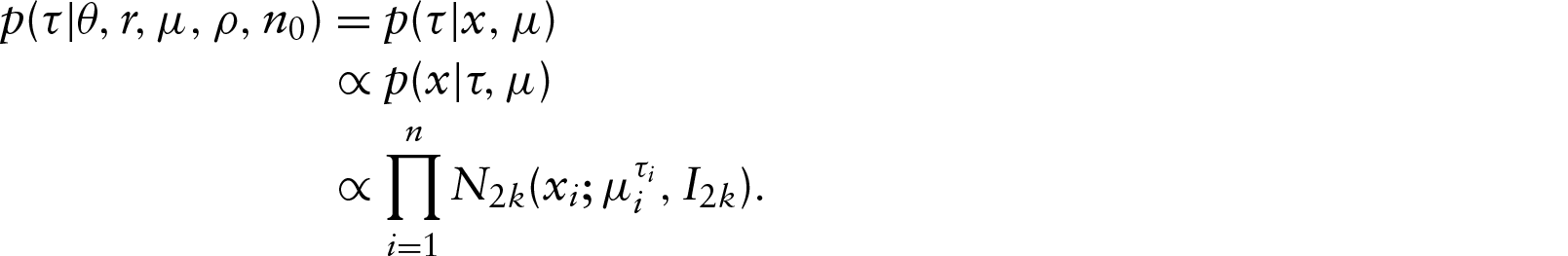
agraph Simulations of r It is shown in the Appendix that the r ij are independent given ( θ , τ , μ , ρ , n 0 ) with density:

p ( r ij | θ , τ , μ , ρ , n 0 ) ∝ r ij e − 1 2 r ij − u ij ′ μ i τ i ( j ) 2 ,

(3.4)

with u ij ′ = ( cos θ ij , sin θ ij ) . If we denote by N 1 + ( m , v ) the univariate normal distribution truncated to [ 0 , ∞ ) , we remark that (3.4) is close to the value of the density of N 1 + ( u ij ′ μ i τ i ( j ) , 1 ) at r ij . It is then natural to simulate from (3.4) by a Metropolis–Hastings step with a N 1 + ( u ij ′ μ i τ i ( j ) , 1 ) as the proposal distribution. Clearly, the probability of acceptance reduces to the ratio min { r ij new / r ij old , 1 } where r ij old and r ij new are, respectively, the current and the proposed values of r ij in the algorithm. Alternative methods of simulations could have been used at this step such as, for example, the slice sampler proposed by Hernandez-Stumpfhauser et al. (2017).

agraph Simulations of τ As the prior distribution of τ is uniform, we have:

p ( τ | θ , r , μ , ρ , n 0 ) = p ( τ | x , μ ) ∝ p ( x | τ , μ ) ∝ ∏ i = 1 n N 2 k ( x i ; μ i τ i , I 2 k ) .

Thus, given ( θ , r , μ , ρ , n 0 ) , the τ i are independent with density (with respect to the counting measure on the set T of permutations of { 1 , … , k } ):

p ( τ i | x , μ ) = N 2 k ( x i ; μ i τ i , I 2 k ) ∑ t ∈ T N 2 k ( x i ; μ i t , I 2 k ) .

(3.5)

agraph Simulations of ρ

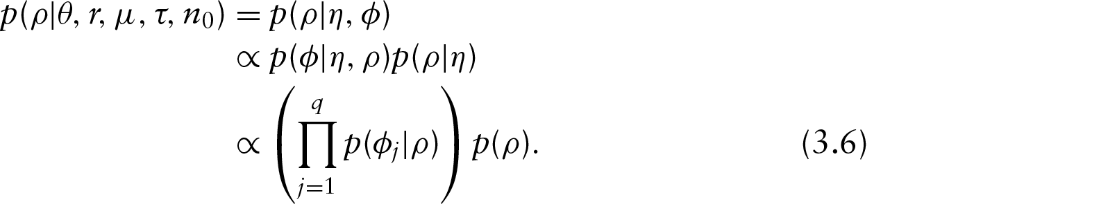
From (2.4), it is clear that the full conditional distribution of ρ reduces to the conditional distribution of ρ given μ . Then, using the parametrization of μ in terms of ( η , ϕ ) and (3.3), we note that η and ρ are independent and that:

p ( ρ | θ , r , μ , τ , n 0 ) = p ( ρ | η , ϕ ) ∝ p ( ϕ | η , ρ ) p ( ρ | η ) ∝ ∏ j = 1 q p ( ϕ j | ρ ) p ( ρ ) .

(3.6)

We show in the Appendix that | Σ 0 − 1 ( ρ ) | = ρ − 2 and that the components of the matrix Σ 0 − 1 ( ρ ) are independent (constant) of ρ except the components of the first 2 by 2 diagonal submatrix (lines and columns 1 and 2). As this submatrix is equal to ( ρ − 1 + ( k − 1 ) ) I 2 , it is easily seen that

ϕ i ′ Σ 0 − 1 ( ρ ) ϕ i = ( ρ − 1 + ( k − 1 ) ) ϕ i 1 ′ ϕ i 1 + constant = ρ − 1 ϕ i 1 ′ ϕ i 1 + constant ,

where ‘constant’ stands for a generic notation for an expression independent of ρ . Since ϕ j | ρ ∼ P 0 ( ρ ) = N 2 k ( 0 , Σ 0 ( ρ ) ) and ρ ∼ IG ( a ρ , b ρ ) , we have:

∏ j = 1 q p ( ϕ j | ρ ) ∝ ρ − q e − 1 2 ρ − 1 ∑ j = 1 q ϕ i 1 ′ ϕ i 1 ,

and it is easy to conclude from (3.6) that the full conditional of ρ is

IG a ρ + q , b ρ + 1 2 ∑ i = 1 q ϕ i 1 ′ ϕ i 1 .

(3.7)

agraph Simulations of n 0 Using the arguments of Escobar and West (1995), under the G ( a n 0 , b n 0 ) prior, n 0 is updated at each Gibbs iteration by sampling first an additional variable ζ from a Beta distribution and then a new value of n 0 from a mixture of Gamma distributions as follows:

ζ | n 0 ∼ B n 0 + 1 , n n 0 | ζ , q ∼ π n G ( a n 0 + q , b n 0 − log ζ ) + ( 1 − π n ) G ( a n 0 + q − 1 , b n 0 − log ζ ) ,

(3.8)

with weights π n defined by π n / ( 1 − π n ) = ( a n 0 + q − 1 ) / [ n ( b n 0 − log ζ ) ] .

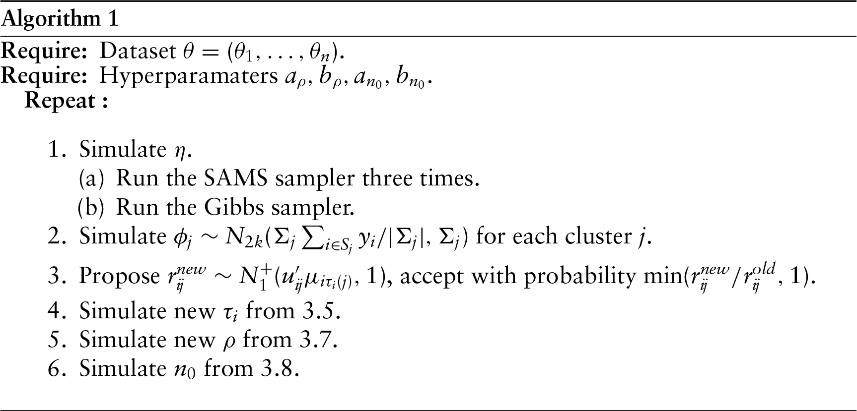
The whole procedure is summarized in Algorithm 1.

OPEN IN VIEWER

Algorithm 1

Require: Dataset θ = θ 1 , … , θ n . Require: Hyperparamaters a ρ , b ρ , a n 0 , b n 0 Repeat: Simulate η (a) Run the SAMS sampler three times. (b) Run the Gibbs sampler. Simulate ϕ j ∼ N 2 k ( Σ j ∑ i ∈ S j y i / | Σ j | , Σ j ) for each cluster j . Propose r ij new ∼ N 1 + ( u ij ′ μ i τ i ( j ) , 1 ) , accept with probability min ( r ij new / r ij old , 1 ) . Simulate new τ i from 3.5. Simulate new ρ from 3.7. Simulate n 0 from 3.8.

To investigate the impact of the symmetrization induced by the variables τ i , we consider a simple model of the following form:

x i | η , ϕ ∼ N 2 k ( ∑ j = 1 q ϕ j 1 { i ∈ S j } , I 2 k ) ϕ j | η ∼ P 0 η ∼ G

(I)

and its symmetrized version:

x i | η , ϕ ∼ N 2 k ( ∑ j = 1 q ϕ j τ i 1 { i ∈ S j } , I 2 k ) ϕ j | η ∼ P 0 η ∼ G τ i ∼ U P ,

(II)

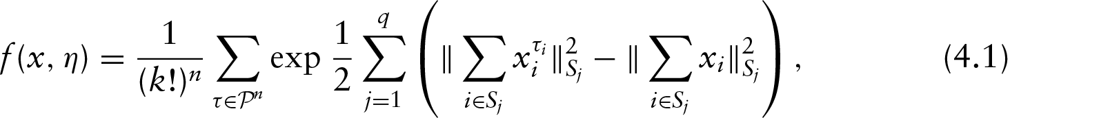
where ϕ j τ i = ( ϕ j τ i ( 1 ) ′ , … , ϕ j τ i ( k ) ′ ) ′ is obtained by random permutation of the coordinates of ϕ j = ( ϕ j 1 ′ , … , ϕ jk ′ ) ′ ∈ ( ℝ 2 ) k . In both models, P 0 = N 2 k ( 0 , Σ 0 ) and G is any distribution of the partition η = { S 1 , … , S q } of { 1 , … , n } . Such distributions include the distribution derived from the Dirichlet process given by (3.3). Model (II) can be viewed as a simplified and reparametrized version of (2.4). Now consider an idealized sample x 1 , … , x n for which every observation x i is simply a random permutation of one unique observation x 0 = ( x 01 ′ , … , x 0 k ′ ) ′ ∈ ( ℝ 2 ) k ; in other words, for every i , there exists a permutation α i such that x i = ( x 0 α i ( 1 ) ′ , … , x 0 α i ( k ) ′ ) ′ . As the coordinates x ij of all the x i are the same but in a different order, it is expected that all the observations are put together in one unique cluster. The aim of this section is to study whether model (4.1) is more appropriate than model (4.1) for this purpose.

Let p 0 and p I ( x | η ) denote respectively the density of P 0 and the conditional density of x = ( x 1 , … , x n ) given η for model (I). We have:

p I ( x | η ) = ∫ ∏ j = 1 q ∏ i ∈ S j N 2 k ( x i ; ϕ j , I 2 k ) p 0 ( ϕ j ) d ϕ j = ∏ j = 1 q m ( x S j ) ,

where x S j = ( x i , i ∈ S j ) and

m ( x S j ) = ∫ ∏ i ∈ S j N 2 k ( x i ; ϕ j , I 2 k ) p 0 ( ϕ j ) d ϕ j .

Denote by p II ( x | η ) the conditional density of x given η for model (II). By (3.1) and noting that { τ i − 1 , τ i ∈ P } = P , we have:

p II ( x | η ) = ∑ τ 1 ( k ! ) n ∫ ∏ j = 1 q ∏ i ∈ S j N 2 k ( x i ; ϕ j τ i , I 2 k ) p 0 ( ϕ j ) d ϕ j = ∑ τ 1 ( k ! ) n ∫ ∏ j = 1 q ∏ i ∈ S j N 2 k ( x i τ i ; ϕ j , I 2 k ) p 0 ( ϕ j ) d ϕ j

= 1 ( k ! ) n ∑ τ ∏ j = 1 q m ( x S j τ ) ,

where the earlier sum is taken for all the values of τ = ( τ 1 , … , τ n ) in P n , x S j τ = ( x i τ i , i ∈ S j ) and x i τ i = ( x i τ i ( 1 ) ′ , … , x i τ i ( k ) ′ ) ′ . Therefore, models (I) and (II) reduce to

x | η ∼ ∏ j = 1 q m ( x S j ) η ∼ G ,

(I’)

and

II ′ x | η ∼ 1 ( k ! ) n ∑ τ ∏ j = 1 q m ( x S j τ ) . η ∼ G .

(II’)

For all partition η = { S 1 , … , S q } and all observation x , we set

f ( x , η ) = 1 ( k ! ) n ∑ τ ∈ P n exp 1 2 ∑ j = 1 q ∥ ∑ i ∈ S j x i τ i ∥ S j 2 − ∥ ∑ i ∈ S j x i ∥ S j 2 ,

(4.1)

where Σ S = Σ 0 − 1 + | S | I 2 k − 1 for all subset S ⊂ { 1 , … , n } and ∥ t ∥ S 2 = t ′ Σ S t for all t ∈ ( ℝ 2 ) k .

Proposition (a) For all partition η = { S 1 , … , S q } and all observation x = ( x 1 , … , x n ) ,

we have:

p II ( x | η ) p I ( x | η ) = f ( x , η ) .

(b) For all distribution G , there exists a positive number B G

such that:

p II ( η | x ) p I ( η | x ) = B G f ( x , η ) ,

for all partition η and all observation x .

(c) For all distribution G , all partition η and all observation x , we have:

p II ( η | x ) p I ( η | x ) ≥ f ( x , η ) 1 max η f ( x , η )

(4.2)

where the maximum is taken over all partitions of { 1 , … , n } .

From ( a ) of Proposition 1, we see that f ( x , η ) is the likelihood ratio of models (II’) and (I’). From ( b ) , we know that the posterior odds ratio is large when f ( x , η ) is large. It would be of interest to know whether this ratio is greater than one. Unfortunately, this is not an easy task except for a few particular cases given further. Indeed, although the factor B G is actually known (see the proof of Proposition 1 in the Appendix), it is rather intractable. From ( c ) , we deduce that the posterior odds is actually greater or equal to one at least for the partition η x that maximizes f ( x , η ) . This partition does exist for any observation x and is independent of G . In other words, for any x , there exists a partition η x such that p II ( η x | x ) ≥ p I ( η x | x ) for all prior G . Finally, we can remark from the proof of the theorem that the equality in (4.2) is obtained when G is a Dirac distribution; a meaningless prior.

Consider the partition η ¯ with a single cluster: q = 1 and S 1 = { 1 , … , n } . From (4.1), the posterior odds ratio when η = η ¯ is likely to be large when ∑ i = 1 n x i ≈ 0 and small when all the x i ≈ x 0 for all i ∈ { 1 , … , n } . Assume from now that ∑ i = 1 n x i = 0 and that Σ 0 = I 2 k . Remember that Σ 0 models the prior information about the mutual positions of the angles on the circle. Therefore, Σ 0 = I 2 k can be viewed as a non-informative prior. In this case, ∥ t ∥ S j 2 = ( 1 + | S j | ) − 1 t ′ t = ( 1 + | S j | ) − 1 ∥ t ∥ for all t ∈ ( ℝ 2 ) k and we have:

f ( x , η ¯ ) = 1 ( k ! ) n ∑ τ ∈ P n exp 1 2 ( n + 1 ) ∥ ∑ i = 1 n x i τ i ∥ 2 .

(4.3)

Example 1 provides a typical sample x = ( x 1 , … , x n ) for which the posterior probability of a unique cluster is greater with model (II) than with model (I) independently of the prior distribution G .

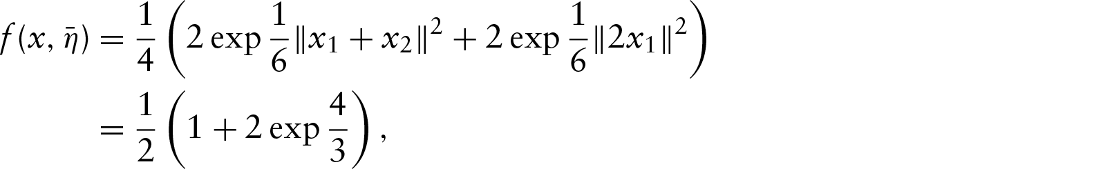
Example 1 First, by noting that:

∑ l = 0 n e il θ = sin θ ( n + 1 ) 2 sin θ 2 e i θ 2 n ,

for all θ ∈ ℝ , we deduce that:

∑ l = 0 k − 1 cos 2 π l k = 0 and ∑ l = 0 k − 1 sin 2 π l k = 0 .

(4.4)

Assume n = k and set x ij = ( cos ( i + j − 2 ) 2 π / k , sin ( i + j − 2 ) 2 π / k ) ′ for i ∈ { 1 , … , k } and j ∈ { 1 , … , k } . In other words, x 1 = ( x 11 ′ , … , x 1 k ′ ) ′ ∈ ( ℝ 2 ) k is made up of k consecutive points on the unit circle separated from an angle of 2 π / k , x 2 is obtained by a rotation with angle 2 π / k of each point of x 1 and so on. Therefore, it is easy to see from (4.4) that ∑ i = 1 n x i = 0 . Our conjecture is that max η f ( x , η ) = f ( x , η ¯ ) for all integer k which implies, from ( c ) of Proposition 1, that the probability of a unique cluster is greater for model (II) than for model (I) for any distribution G . For n = k = 2 the conjecture reduces to f ( x , η ) ≤ f ( x , η ¯ ) for a single partition η = { { x 1 } , { x 2 } } . As ∥ x i ∥ S j = ∥ x i τ i ∥ S j for all i and τ i , it is easily seen from (4.1) that f ( x , η ) = 1 . On the other hand, as ∥ x 1 ∥ 2 = k and x 1 = − x 2 , we see from (4.3) that

f ( x , η ¯ ) = 1 4 2 exp 1 6 ∥ x 1 + x 2 ∥ 2 + 2 exp 1 6 ∥ 2 x 1 ∥ 2 = 1 2 1 + 2 exp 4 3 ,

hence the proof of the conjecture for n = k = 2 . We also proved the conjecture for n = k = 3 with a rather large amount of calculations (not given here) to take into account all the partitions η and all the permutation τ = ( τ 1 , τ 2 , τ 3 ) . We are not in a position to provide general proof of the conjecture for n = k ≥ 4 .

With small datasets, a misspecification of the prior could have a strong negative impact on the final results. Therefore, special attention has to be paid to the prior and the hyperparameter specifications. Consequently, we test our algorithm on two simulation studies to evaluate the influence of some hyperparameters.

The performances of our method are investigated using the adjusted Rand index (ARI), proposed by Hubert and Arabie (1985), to compare our obtained partition to the actual one. The Rand index (Rand, 1971) is a well-known measure of the similarity between two partitions. If we denote by N 00 the numbers of pairs that are in the same cluster in both partitions and by N 11 the number of pairs that are in different clusters in both partitions, then the Rand index is defined by the ratio ( N 00 + N 11 ) / ( 2 n ) . The ARI is a corrected-for-chance version of the Rand index. Its expected value (under the generalized hypergeometric model) is equal to 0 and its maximum is 1, while the expected value of the Rand index depends on the number of clusters. For a presentation of the different criteria for clustering comparison and for a study investigating the usefulness of the adjusted measures, we refer the reader to Fritsch and Ickstadt (2009) and Nguyen et al. (2009).

5.1 Influence of the precision parameter ρ

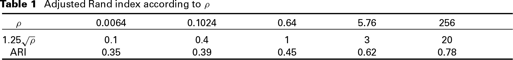
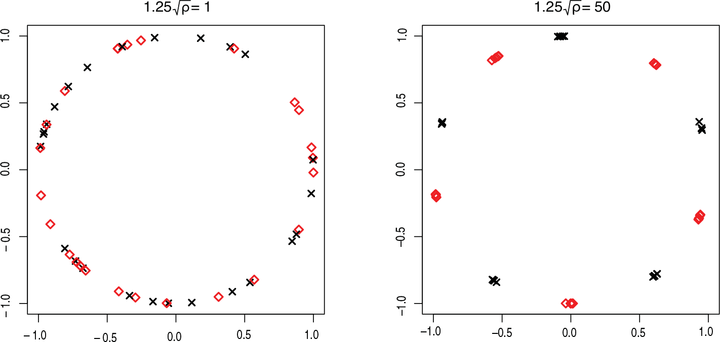
First, we choose to simulate data using a procedure which is close to our model in order to investigate the influence of the precision parameter ρ . We set q = 3 clusters of 10 data. We simulate the coordinates μ ij of each centre μ i approximately on a circle with a fixed radius. Since it is shown in Section 2 that E ∥ μ i 1 ∥ = ρ π / 2 ≈ 1.25 ρ , the first coordinate μ i 1 is simulated according to a uniform distribution on the circle with radius 1.25 ρ . The other coordinates μ ij , j = 2 , … , 5 ( k = 5 ) are generated according to a noisy rotation with angle 2 π j / 5 of μ i 1 . For each cluster i , we generate 10 data according to PN 10 ( μ i , I 10 ) . A comparison of the generated data is provided in Figure 2 with different values for ρ ; for the clarity of the picture, we choose to represent only q = 2 clusters of 5 observations. It is clear from Figure 2 that large values of ρ provide small variability for the projected observations. This observation can be confirmed by a simulation study. We simulate some datasets according to the earlier procedure with different values for ρ . For each value of ρ , a hundred datasets are simulated. Then, our Bayesian methodology is applied using a n 0 = 10 and b n 0 = 1 . The mean values for the ARI are given in Table 1.

OPEN IN VIEWER

Table 1:

Adjusted Rand index according to ρ

ρ	0.0064	0.1024	0.64	5.76	256
1.25 ρ	0.1	0.4	1	3	20
ARI	0.35	0.39	0.45	0.62	0.78

As expected, this parameter has an important influence on the obtained results. We choose a non-informative prior for ρ by setting a ρ = b ρ = 0.01 . This prior is close to the Jeffreys prior for the model N 2 ( 0 , ρ I 2 ) whose density reduces to ρ − 1 .

OPEN IN VIEWER Figure 2:

Two datasets are generated with two different values for the parameter ρ to highlight the influence of this parameter. Two clusters of five data are represented on each plot. Each data is composed of k = 5 angles on the circle. One cluster is represented by the black cross, the other by the red square

5.2 Robustness to the Hperparameters a n 0 and b n 0

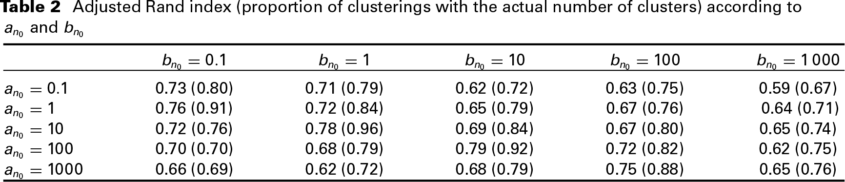
It is well known that the number of clusters does depend on n 0 whose prior distribution is fixed by the hyperparameters a n 0 and b n 0 . In this subsection, we investigate the sensitivity of the ARI with respect to these hyperparameters. We apply the same simulation strategy as in the previous subsection with a fixed value of ρ such that 1.25 ρ = 20 . Note that the parameters a n 0 and b n 0 are not at all involved in the simulation of the dataset. The mean values for the ARI over 100 simulated datasets are given in Table 2.

OPEN IN VIEWER

Table 2:

Adjusted Rand index (proportion of clusterings with the actual number of clusters) according to a n 0 and b n 0

	b n 0 = 0.1	b n 0 = 1	b n 0 = 10	b n 0 = 100	b n 0 = 1 000
a n 0 = 0.1	0.73 (0.80)	0.71 (0.79)	0.62 (0.72)	0.63 (0.75)	0.59 (0.67)
a n 0 = 1	0.76 (0.91)	0.72 (0.84)	0.65 (0.79)	0.67 (0.76)	0.64 (0.71)
a n 0 = 10	0.72 (0.76)	0.78 (0.96)	0.69 (0.84)	0.67 (0.80)	0.65 (0.74)
a n 0 = 100	0.70 (0.70)	0.68 (0.79)	0.79 (0.92)	0.72 (0.82)	0.62 (0.75)
a n 0 = 1000	0.66 (0.69)	0.62 (0.72)	0.68 (0.79)	0.75 (0.88)	0.65 (0.76)

Table 2 suggests that a choice of a n 0 / b n 0 approximately between 1 and 10 provides good and similar results.

5.3 Influence of the number of clusters

Using the previously fixed hyperparameters, a simulation study is provided with different numbers of clusters. For each number of clusters, 100 datasets are simulated according to the earlier procedure. Each cluster has a number of points randomly chosen between 10 and 20 . The results are gathered in Table 3.

OPEN IN VIEWER

Table 3:

Adjusted Rand index according to the number of clusters

Number of clusters	1	3	5	8	10
ARI	0.97	0.74	0.71	0.66	0.60

The results are rather good even with a high number of clusters.

OPEN IN VIEWER Figure 3:

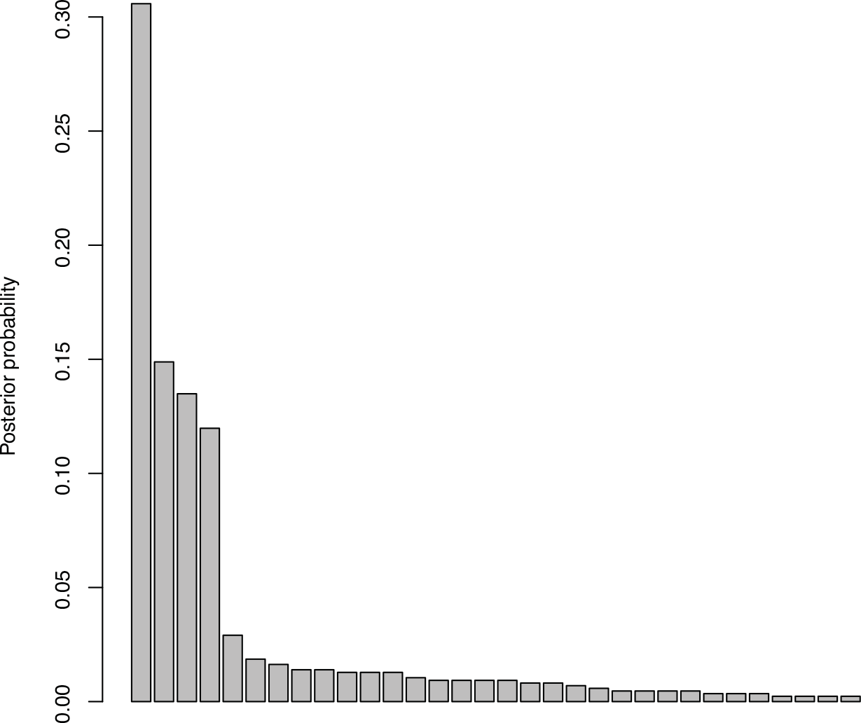
Barplot of the proportion of 32 more probable clusterings. For a better apprehension, the clusterings that have a posterior probability lower than 0.02% have been omitted

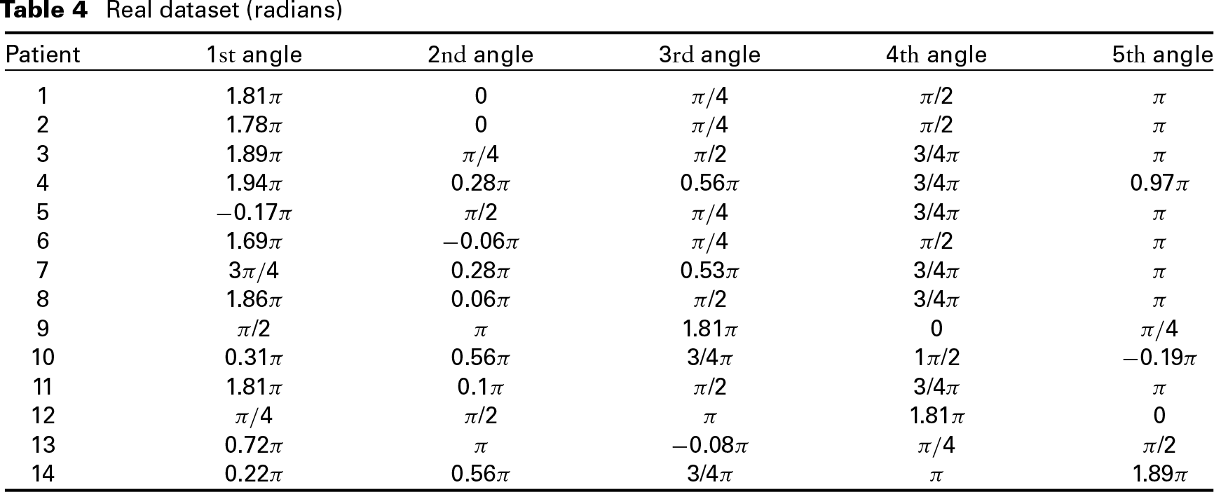
We then apply the methodology to a real dataset from post-operative treatment of liver cancer at the Institute of Sainte Catherine in Avignon, France (see Figure 1 and Table 4). Let us recall that no other competing methods exist for these kind of multivariate circular data except the method described in Abraham et al. (2013) with a fixed number of clusters. Consequently, our results are compared to those of Abraham et al. (2013) in which the number of clusters was preselected to q = 2 .

Let us remind you that the a priori distribution of n 0 is a gamma distribution with parameter a n 0 and b n 0 with an expected value equal to a n 0 / b n 0 (if a n 0 > 1 ) and a variance equal to a n 0 / b n 0 2 (if a n 0 > 2 ). Remember that the expected number of clusters given n 0 is approximately equal to n 0 log ( 1 + n / n 0 ) (Teh, 2010). According to the results of Section 5, the results are robust with respect to the choice of the hyperparameters a n 0 and b n 0 with 1 ≤ a n 0 / b n 0 ≤ 10 . We choose a rather non-informative prior by setting a n 0 = 3 and b n 0 = 0.3 which leads to a distribution of n 0 centred around 3 with a large variance. Other values for a n 0 and b n 0 have been tested and give nearly the same results. As in Section 5, we choose a non-informative prior by setting a ρ = b ρ = 0.01 .

OPEN IN VIEWER

Figure 4:

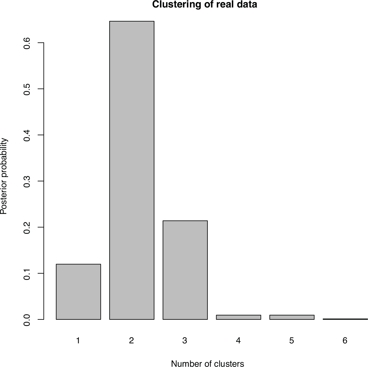
Posterior distribution of the number of clusters

MCMC convergence diagnostics was investigated with the clustering entropy

− ∑ i = 1 q | S i | n log | S i | n .

Traceplots for this quantity and for other parameters of the model suggest a good mixing and the convergence of our chain. On a classical personal laptop and using a nonoptimized code, the time of mixing was approximately 12 minutes, whereas the whole procedure lasts 90 minutes.

The majority clustering (mode of the posterior distribution of the clusterings) is the same as in Abraham et al. (2013) (two clusters: one containing data 1, 2, 6, 9 and 12, the second containing data 3, 4, 5, 7, 8, 10, 11, 13 and 14) with a posterior probability equal to 30.5%. This result was awaited and is coherent with the choice of 2 clusters in the previous method. But the real gain from our Bayesian approach is to look beyond this majority clustering. Here there are 3 more clusterings that are significant and that could give some information on this real dataset. The second majority clustering is nearly the same as the previous one: the clusters are the same but data 6 is alone in a third cluster. Indeed, this data is very atypical because it is the only one that contains an angle near 1.69 π . The posterior probability for this clustering is 14.9%. The third majority clustering gives nearly the same information with a posterior probability of 13.5%. There are two clusters: one with data 6 and a second with all the others. Finally, another clustering with a posterior probability of 12.0% is made up of only one cluster. Even with other choices for the hyperparameters a n 0 and b n 0 , the posterior probability of this clustering remains high. It highlights the fact that all the data share some common traits and the main difference in the two clusters of the majority clustering only concerns one angle. All the clusterings are included in Figure 3 sorted by their posterior probabilities. It can be noted that a credible region with a posterior probability of 71% is composed of the four previous clusterings.

We give in Figure 4 the posterior distribution of the number of clusters. The posterior probabilities of 1, 2 or 3 clusters are respectively 12%, 65% and 21%. Consequently, the number of clusters is certainly (with probability 98%) less than or equal to 3.

As expected, these results are in line with the clusterings obtained in Abraham et al. (2013). The final choice of two clusters (that is not made here a priori) could provide, using the centres of the clusters, preset positions for praticians. As explained earlier, these two centres share only one main difference on one unique angle. This is highlighted by the important posterior probability of the clustering with only one cluster. Thus, using these preset positions should be fairly easy for praticians, with four fixed values and only two choices for the last one. Furthermore, the results suggest another preset position that should be added and tested if the two previous one do not fit: the beam angles of data 6. As explained in Yuan et al. (2015), the definition of such presets will help to save time (at least 30 minutes for each patient) and will allow more people to be treated with this technology; it is also shown that the beams generated with our methodology show dosimetric qualities comparable to their manually generated clinical counterpart, even if no adjustments were allowed around the fixed presettings.

OPEN IN VIEWER

Table 4:

Real dataset (radians)

Patient	1 st angle	2 nd angle	3 rd angle	4 th angle	5 th angle
1	1.81 π	0	π / 4	π /2	π
2	1.78 π	0	π / 4	π /2	π
3	1.89 π	π / 4	π /2	3/4 π	π
4	1.94 π	0.28 π	0.56 π	3/4 π	0.97 π
5	− 0.17 π	π /2	π / 4	3/4 π	π
6	1.69 π	− 0.06 π	π / 4	π /2	π
7	3 π / 4	0.28 π	0.53 π	3/4 π	π
8	1.86 π	0.06 π	π /2	3/4 π	π
9	π /2	π	1.81 π	0	π / 4
10	0.31 π	0.56 π	3/4 π	1 π /2	− 0.19 π
11	1.81 π	0.1 π	π /2	3/4 π	π
12	π / 4	π /2	π	1.81 π	0
13	0.72 π	π	− 0.08 π	π / 4	π /2
14	0.22 π	0.56 π	3/4 π	π	1.89 π

We present a full Bayesian framework for the clustering of multivariate circular and non-ordered data. It is based on a hierarchical model that combines projected normal distributions and the Dirichlet Process. Two original parameters are also introduced in this model: the parameter ρ to infer the variance of the angles and the symmetrization parameter τ to model the non-ordered feature of the data. The parameters of the model are then inferred using a Metropolis–Hastings-within-Gibbs algorithm and a theoretical study of the impact of the symmetrization parameter is provided. The simulation study and the real data example show the benefits of this approach. Indeed, the number of clusters is chosen automatically by the method and the final result is much more complete than the majority clustering which is usually provided by classical clustering algorithms. However, some improvements could be considered, such as incorporating covariates (shape or size of the tumour, stage of the cancer, sex, age,...) to preselect the beam positions.

Declaration of conflicting interests

The authors declared no potential conflicts of interest with respect to the research, authorship and/or publication of this article.

Funding

The authors received no financial support for the research, authorship and/or publication of this article.

Supplementary material

Supplementary Material containing the Appendix is available from http://www.statmod.org/smij/archive.html.