Combining historical data and bookmakers’ odds in modelling football scores

Abstract

Modelling football outcomes has gained increasing attention, in large part due to the potential for making substantial profits. Despite the strong connection existing between football models and the bookmakers’ betting odds, no authors have used the latter for improving the fit and the predictive accuracy of these models. We have developed a hierarchical Bayesian Poisson model in which the scoring rates of the teams are convex combinations of parameters estimated from historical data and the additional source of the betting odds. We apply our analysis to a nine-year dataset of the most popular European leagues in order to predict match outcomes for their tenth seasons. In this article, we provide numerical and graphical checks for our model.

Keywords

Bayesian Poisson model betting odd football prediction historical results model checks

1 Introduction

In recent years, the challenge of modelling football outcomes has gained attention, in large part due to the potential for making substantial profits in betting markets. This task may be achieved by adopting two different modelling strategies: the ‘direct’ models, for the number of goals scored by two competing teams; and the ‘indirect’ models, for estimating the probablility of the categorical outcome of a win, a draw, or a loss, which will hereafter be referred to as a ‘three-way’ process.

The basic assumption of the direct models is that the number of goals scored by the two teams follow two Poisson distributions. Their dependence structure and the specification of their parameters are the other most relevant assumptions, according to the literature. The scores’ (goals’) dependence issue is, in fact, the subject of much debate, and the discussion cannot yet be concluded. As one of the first contributors to the modelling of football scores, Maher (1982) used two conditionally independent Poisson distributions, one for the goals scored by the home team, and another for the away team. Dixon and Coles (1997) expanded upon Maher's work and extended his model, introducing a parametric dependence between the scores. This also represents the justification for the bivariate Poisson model, introduced in Karlis and Ntzoufras (2003) in a frequentist perspective, and in Ntzoufras (2011) under a Bayesian perspective. On the other hand, Baio and Blangiardo (2010) assume conditional independence within hierarchical Bayesian models, on the grounds that the correlation of the goals is already taken into account by the hierarchical structure. Similarly, Groll and Abedieh (2013) and Groll et al. (2015) show that, up to a certain amount, the scores’ dependence on two competing teams may be explained by the inclusion of some specific team covariates in the linear predictors. However, Dixon and Robinson (1998) note that modelling the dependence along a single match is possible: in such a case, a temporal structure in the 90 minutes is required.

The second common assumption is the inclusion in the models of some teams’ effects to describe the attack and the defence strengths of the competing teams. Generally, they are used for modelling the scoring rate of a given team, and in much of the aforementioned literature they do not vary overtime. Of course, this is a major limitation. Dixon and Coles (1997) tried to overcome this problem by downweighting the likelihood exponentially overtime in order to reduce the impact of matches far from the current time. However, over the last 10 years the advent of some dynamic models allowed these teams’ effects to vary over the seasons, and to have a temporal structure. The independent (or double) Poisson model proposed by Maher (1982) has been extended to a Bayesian dynamic independent model, where the evolution structure is based on continuous time (Rue and Salvesen, 2000), or is specified for discrete times, such as a random walk for both the attack and defence parameters (Owen, 2011). Instead, the non-dynamic bivariate Poisson model is extended in Koopman and Lit (2015) and Koopman et al. (2017), and is expressed as a state space model where the teams’ effects vary in function of a state vector.

For our purposes, the scores’ dependence assumption may be relaxed, and in this article we assume conditional independence. From a purely conceptual point of view, we have several reasons for adopting two independent Poisson: (a) as discussed by Baio and Blangiardo (2010), assuming two conditionally independent Poisson hierarchical Bayesian models implicitly allows for correlation, since the observable variables are mixed at an upper level; (b) as noted by McHale and Scarf (2011), there is empirical evidence that goals of two teams in seasonal leagues display only slightly positive correlation, or no correlation at all, where as goals are negatively correlated for national teams; (c) bivariate Poisson models (Karlis and Ntzoufras, 2003), which represent the most typical choice for modelling correlation, only allow for non-negative correlation. Moreover, the independence assumption allows for a simpler formulation for the likelihood function and simplifies the inclusion of the bookmakers’ odds in our model. Concerning the dynamic assumption of the team-specific effects, we use an autoregressive model by centring the effect of seasonal time $τ$ at the lagged effect in $τ - 1$ , plus a fixed effect.

Whatever the choices for the two assumptions discussed earlier, the models proposed in this context were built with both a descriptive and a predictive goal, and their parameters’ estimates/model probabilities were often used for building efficient betting strategies (Dixon and Coles (1997); Londono and Hassan, 2015). In fact, the well-known expression ‘beating the bookmakers’ is often considered a mantra for whoever tries to predict football—or more generally, sports—results. As mentioned by Dixon and Coles (1997), to win money from the bookmakers requires a determination of probabilities, which is sufficiently more accurate than those obtained from the odds. On the other hand, it is empirically known that odds of the bookies are the most accurate source of information for forecasting sports performances (Štrumbelj, 2014). However, at least two issues deserve a deep analysis: how to determine probability forecasts from the raw betting odds, and how to use this source of information within a forecasting model (e.g., to predict the number of goals). Concerning the first point, it is well known that the betting odds do not correspond directly to probabilities; in fact, to make a profit, bookmakers set unfair odds, and they have a ‘take’ of 5–10%. In order to derive a set of coherent probabilities from these odds, many researchers have used the ‘basic normalization’ procedure, by normalizing the inverse odds up to their sum. Alternatively, Forrest et al. (2005) and Forrest and Simmons (2000) propose a model-based approach, where the betting probabilities are the dependent variables of a regression model, with a historical set of betting odds and match outcomes as independent variables. However, Štrumbelj (2014) shows that Shins procedure (Shin, 1991, 1993) gives the best results overall, being preferable both to the basic normalization and regression approaches. Concerning the second issue, a small amount of literature focused on using the existing betting odds as ‘part’ of a statistical model for improving the predictive accuracy and the model fit. Londono and Hassan, 2015 use the betting odds for eliciting the hyperparameters of a Dirichlet distribution, and then update them based on observations of the categorical three-way process. No researcher has tried to implement a similar strategy within the framework of direct models.

In this article we try to fill the gap, creating a bridge between the betting odds and betting probabilities, on the one hand, and the statistical modelling of the scores, on the other hand. After transforming the inverse betting odds into probabilities, we develop a procedure to (a) infer from these the implicit scoring intensities, according to the bookmakers, and (b) use these implicit intensities directly in the conditionally independent Poisson model for the scores, within a Bayesian perspective. We are interested in both the estimation of the models parameters, and in the prediction of a new set of matches. Intuitively, the latter task is much more difficult than the former, since football is intrinsically noisy and hardly predictable. However, we believe that combining the betting odds with an historical set of data on match results may give predictions that are more accurate than those obtained from a single source of information.

In Section 2, we introduce two methods, proposed in the literature, for transforming the three-way betting odds favoured by bookmakers into probabilities. In Section 3, we introduce the full model, along with the implicit scoring rates. The results and predictive accuracy of the model on the top four European leagues—Bundesliga, Premier League, La Liga and Serie A—are presented in Section 4, and are summarized through posterior probabilities and graphical checks. Moreover, some model assumptions are checked via predictive measures. Some profitable betting strategies are briefly presented in Section 5. Section 6 concludes our analysis.

2 Transforming the betting odds into probabilities

The connection between betting odds and probabilities has been broadly investigated over the last decades. The odds of any given event are usually specified as the amount of money we would win if we bet one unit on that event. The inverse odds—usually denoted as 1:2.5—correspond to the imprecise probability associated to that event. In fact, as is widely known, the betting odds do not correspond directly to precise probabilities: the sum of the inverse odds for a single match needs to be greater than one (Dixon and Coles (1997)) in order to guarantee the bookmakers’ profit. Here, $o_{m} = {o_{w i m}, o_{D r a w}, o_{l o s s}}, Π_{m} = (π_{w i m}, π_{D r a w}, π_{L o s s}), a n d Δ_{m} = {' W i n',' D r a w',' L o s s'}$ denote the vector of the inverse betting odds, the vector of the estimated betting probabilities and the set of the three-way possible results for the $m$ th game, respectively.

There is empirical evidence that the betting odds are the most accurate available source of probability forecasts for sports (Štrumbelj, 2014); in other words, forecasts based on odds probabilities have been shown to be better, or at least as good as, statistical models, which use sport-specific predictors and/or expert tipsters.

However, some issues remain open. Among these, there is a strong debate over which method to use for inferring a set of probabilities from the raw betting odds. We can transform them into probabilities by using the two procedures proposed in the literature: the ‘basic normalisation’—dividing the inverse odds by the booksum, that is, the sum of the inverse betting odds, as broadly explained in Štrumbelj (2014)—and ‘Shin's procedure’ described in Shin (1991, 1993). Štrumbelj (2014), Cain et al. (2002, 2003), and Smith et al. (2009) show that Shins probabilities improve over the basic normalization: In Štrumbelj (2014), this result has been achieved by the application of the ranked probability score (RPS; Epstein, 1969), which may be defined as a discrepancy measure between the probability of a three-way process outcome and the actual outcome.

In this article we will not focus on comparing these two procedures; rather, we are interested in using the probabilities derived from each of them for statistical and prediction purposes, as will become clearer in later sections.

(A) Basic normalization

π_{i} = \frac{o_{i}}{β}, i \in Δ_{m},

(2.1)

where $β = \sum_{i} o_{i}$ is the so called booksum (Štrumbelj, 2014). The method has gained a great popularity due to its simplicity.

(B) Shin's procedure

In the model proposed by Shin (1993), the bookmakers specify their odds in order to maximize their expected profit in a market with uninformed bettors and insider traders. The latter are those particular actors who, due to superior information, are assumed to ‘already’ know the outcome of a given event—for example, football match, horse race, etc.—before the event takes place. Their contribution in the global betting volume is quantified by the percentage $z$ . Jullien et al. (1994) use Shin's model to explicitly work out the expression for the betting probabilities:

π (z)_{i} = \frac{\sqrt{z^{2} + 4 (1 - z) \frac{o_{i}^{2}}{\sum_{i} o_{i}}} - z}{2 (1 - z)}, i \in Δ_{m} .

(2.2)

The current literature refers to these as Shin's probabilities. The earlier formula is a function depending on the insider trading rate $z$ , which Jullien et al. (1994) suggested should be estimated by nonlinear least squares as:

Argmin {\sum_{i = 1}^{3} π {(z)}_{i} - 1} .

The value obtained here may be defined as the minimum rate of insider traders that yields probabilities corresponding to the vector of inverse betting odds $O$ .

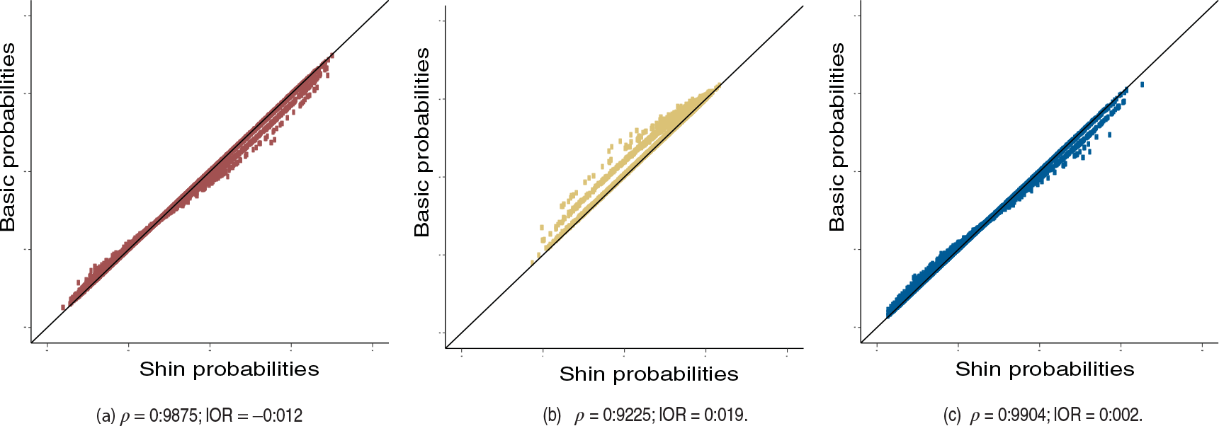
Figure 1 displays the three-way betting probabilities obtained through the two procedures described earlier for English Premier League, from the season 2007–2008 to the season 2016–2017; the single captions report the Pearson's correlation coefficients and a global log-odds ratio. As may be noted, the draw probabilities obtained with the basic normalization tend to be higher than those obtained with Shin's procedure. Conversely, as a home win and an away win tend to become more likely, Shin's procedure tends to favour them.

Figure 1:

Comparison between home (Panel (a)), draw (Panel (b)) and loss (Panel(c)) Shin probabilities ( $x$ -axis) and the corresponding basic normalized probabilities ( $y$ -axis) for the English Premier League (seasons from 2007–2008 to 2016–2017), according to seven different bookmakers. For each three-way outcome, $ρ$ is the Pearson's correlation coefficient and $lOR$ a global log-odds ratio between basic and Shin probabilities over all the matches and all the different bookmakers

3 Model

3.1 Model for the scores

Here, $y = (y_{m 1}, y_{m 2})$ denotes the vector of observed scores, where $y_{m 1}$ and $y_{m 2}$ are the number of goals scored by the home team and by the away team, respectively, in the $m$ th match of the dataset. Following Baio and Blangiardo (2010), we adopt a conditional independence assumption between the scores. This choice allows for a simpler formulation for the likelihood function and, later on, for the direct inclusion of the bookies odds into the model through the Skellam distribution ( Karlis and Ntzoufras, 2009). The model for the scores is then specified as:

\begin{matrix} \begin{matrix} y_{m 1} | θ_{m 1} & \sim Poisson (θ_{m 1}) \\ y_{m 2} | θ_{m 2} & \sim Poisson (θ_{m 2}), \\ y_{m 1} ⊥ & y_{m 2} | θ_{m 1}, θ_{m 2}, \end{matrix} \end{matrix}

(3.1)

where $y$ is modelled as ‘conditionally’ independent Poisson and the joint parameter $θ = (θ_{m 1}, θ_{m 2})$ represents the scoring intensities in the $m$ th game, for the home team, and for the away team, respectively. In what follows, we will refer to (3.1) as the ‘basic’ model, which is estimated using the past scores. The main novelty of this article consists of enriching this specification by including the extra information which stems from the betting odds. Thus, for each pair of match $m$ and bookmaker $s$ , the betting probabilities $π_{i, m}^{s}, i \in Δ_{m}$ , derived with one of the methods in Section 2, may be used to find out the values ${\hat{θ}}^{s} = ({\hat{θ}}_{m 1}^{s}, {\hat{θ}}_{m 2}^{s})$ , which solve the following nonlinear system of equations:

\begin{matrix} \begin{matrix} π_{Win, m}^{s} + π_{Draw, m}^{s} = & P (y_{m 1} \geq y_{m 2} | θ_{m 1}^{s}, θ_{m 2}^{s}) \\ π_{Loss, m}^{s} = & P (y_{m 1} < y_{m 2} | θ_{m 1}^{s}, θ_{m 2}^{s}) . \end{matrix} \end{matrix}

(3.2)

The existence of these values is guaranteed by the fact that, under (3.1),

y_{m 1} - y_{m 2} \sim PD (θ_{m 1}, θ_{m 2})

, where

PD

denotes the Poisson difference distribution, also known as Skellam distribution, with parameters

θ_{m 1}, θ_{m 2}

and mean

θ_{m 1} - θ_{m 2}

. In such a way, we obtain for each pair

(m, s)

the ‘implicit’ scoring rates

{\hat{θ}}_{m 1}^{s}, {\hat{θ}}_{m 2}^{s}

, somehow inferring the scoring intensities implicit in the three-way bookies odds. Now, we consider our augmented dataset by including as auxiliary data the observed

{\hat{θ}}_{m 1}^{s}, {\hat{θ}}_{m 2}^{s}

. For every

m

, our new data vector is represented by:

(y, {\hat{θ}}^{s}) = (y_{m 1}, y_{m 2}, {\hat{θ}}_{m 1}^{s}, {\hat{θ}}_{m 2}^{s}, s = 1, \dots, S) .

Now, from Equation (3.1) we move to the following specification:

\begin{matrix} \begin{matrix} y_{m 1} | θ_{m 1}, λ_{m 1} & \sim Poisson (p_{m} θ_{m 1} + (1 - p_{m}) λ_{m 1}) \\ y_{m 2} | θ_{m 2}, λ_{m 2} & \sim Poisson (p_{m} θ_{m 2} + (1 - p_{m}) λ_{m 2}), \end{matrix} \end{matrix}

(3.3)

where $λ_{m 1}, λ_{m 2}$ are bookmakers’ parameters introduced for modelling the additional data ${\hat{θ}}_{m 1}^{s}, {\hat{θ}}_{m 2}^{s}, s = 1, \dots, S$ , as explained in the next section. The mixing parameter $p_{m}$ is assigned a non-informative prior distribution, with hyper-parameters $a$ and $b$ , for example, $p_{m} \sim Beta (a, b)$ .

The model introduced in (3.3) still relies on the conditional independence assumption, but the rates are now convex combinations accounting for different information sources. Roughly speaking, this approach presents some similarities with the Bayesian model averaging perspective (Hoeting et al., 1999), with the first model $M_{1}$ driven by the data and the second $M_{2}$ by the bookies odds. A pure BMA approach weights the posterior distributions of each model by the posterior model probabilities—accounting then for model uncertainty—where as our procedure directly weights the two separate match-specific sources of information in the model itself.

3.2 Model for the rates

Equation (3.3) introduced a convex combination for the Poisson parameters, accounting for both the scoring rates $θ_{\cdot 1}, θ_{\cdot 2}$ and the bookmakers’ parameters $λ_{\cdot 1}, λ_{\cdot 2}$ . Denoting with $T$ the number of teams, the common specification for the scoring intensities is a log-linear model in which for each $t, t = 1, \dots, T$ :

\begin{matrix} \begin{matrix} \log (θ_{m 1}) & = μ + home + {att}_{t [m] 1} + {def}_{t [m] 2} \\ \log (θ_{m 2}) & = μ + {att}_{t [m] 2} + {def}_{t [m] 1}, \end{matrix} \end{matrix}

(3.4)

with the nested index

t [m]

denoting the team

t

in the

m

th game.

μ

is the global intercept, while the parameter ‘home’ represents the well-known football advantage of playing at home, and is assumed to be constant for all the teams overtime, as in the current literature. The attack and defence strengths of the competing teams are modelled by the parameters

att

and

def

, respectively. Baio and Blangiardo (2010) and Dixon and Coles (1997) assume that these team-specific effects do not vary over the time, and this represents a major limitation in their models. In fact, Dixon and Robinson (1998) show that the attack and defence effects are not static and may even vary during a single match; thus, a static assumption is often not reliable for making predictions and represents a crude approximation of the reality. Rue and Salvesen (2000) propose a generalized linear Bayesian model in which the team-effects at match time

τ

are drawn from a normal distribution centred at the team-effects at match time

τ - 1

, and with a variance term depending on the time difference. We adopt an intermediate strategy in which attack and defence parameters are allowed to vary between seasons, considering the effects for the season

τ

following a normal distribution centred at the previous seasonal effect plus a fixed component. For each

t = 1, \dots, T, τ = 2, \dots, T

\begin{matrix} \begin{matrix} {att}_{t, τ} & \sim N (μ_{att} + {att}_{t, τ - 1}, σ_{att}^{2}) \\ {def}_{t, τ} & \sim N (μ_{def} + {def}_{t, τ - 1}, σ_{def}^{2}), \end{matrix} \end{matrix}

(3.5)

while, for the first season, we assume:

\begin{matrix} \begin{matrix} {att}_{t, 1} & \sim N (μ_{att}, σ_{att}^{2}) \\ {def}_{t, 1} & \sim N (μ_{def}, σ_{def}^{2}) . \end{matrix} \end{matrix}

(3.6)

As outlined in the literature, we need to impose a ‘zero-sum’ identifiability constraint within each season to these random effects:

\sum_{t = 1}^{T} {att}_{t, τ} = 0, \sum_{t = 1}^{T} {def}_{t, τ} = 0, τ = 1, \dots T,

where as $μ$ and the hyperparameters of our model are assigned weakly informative and non-informative priors:

\begin{matrix} μ, home, μ_{att}, μ_{def} \sim & N (0, 10) \\ σ_{att}^{2}, σ_{def}^{2} \sim & InvGamma (0.001, 0.001), \end{matrix}

where $InvGamma$ denotes the inverse Gamma distribution. The team-specific effects modelled through Equations (3.5) and (3.6) are estimated from the past scores in the dataset. As expressed in (3.3), we add a level to the hierarchy, by including the implicit scoring rates as a separate data model. Given, then, a further level which consists of $S$ bookmakers, it is natural to consider $λ_{m 1}, λ_{m 2}$ as the model parameters for the observed ${\hat{θ}}_{m 1}^{s}, {\hat{θ}}_{m 2}^{s}$ . More precisely, these parameters represent the means of two lognormal distributions for the further implicit scoring rates model:

\begin{matrix} \begin{matrix} {\hat{θ}}_{m 1}^{1}, \dots, {\hat{θ}}_{m 1}^{S} & \sim Lognormal (λ_{m 1}, τ_{1}^{2}) \\ {\hat{θ}}_{m 2}^{1}, \dots, {\hat{θ}}_{m 2}^{S} & \sim Lognormal (λ_{m 2}, τ_{2}^{2}), \end{matrix} \end{matrix}

(3.7)

where $Lognormal (μ, σ^{2})$ is the lognormal distribution with parameters $μ \in ℝ, σ^{2} \in ℝ^{+}$ . $λ_{m 1}, λ_{m 2}$ are in turn assigned two lognormal distributions with hyperparameters $α_{1}, α_{2}$ :

\begin{matrix} \begin{matrix} λ_{m 1} & \sim Lognormal (α_{1}, 10) \\ λ_{m 2} & \sim Lognormal (α_{2}, 10) . \end{matrix} \end{matrix}

(3.8)

4 Applications and results: Top four European leagues

4.1 Data

We collect the exact scores for the top four European professional leagues—Italian Serie A, English Premier League (hereafter, EPL), German Bundesliga, and Spanish La Liga—from season 2007–2008 to 2016–2017. Moreover, we also collected all the three-way odds for the following bookmakers: Bet365, Bet&Win, Interwetten, Ladbrokes, Sportingbet, VC Bet, William Hill. All these data have been downloaded from the public available page http://www.football-data.co.uk/. We are interested in both (a) posterior predictive checks in terms of replicated data under our models, and (b) out-of-sample predictions for a new dataset. According to point (b), which appears to be more appealing for fans, bettors and statisticians, let $T_{r}$ denote the ‘training set’, and $T_{s}$ the ‘test set’. Our training set contains the results of nine seasons for each professional league, and our test set contains the results of the tenth season. The model coding has been implemented in JAGS (Plummer, 2017)—see the supplementary material for the model code. We ran our MCMC simulation for $H = 5 000$ iterations, with a burn-in period of $1 000$ , and we monitored the convergence using the usual MCMC diagnostic (Gelman et al., 2014).

4.2 Parameter estimates

As broadly explained in Section 3, the model in (3.3) combines historical information about the scores and betting information about the odds. We acknowledge that the scoring rate is a convex combination that ‘borrows strengths’ from both sources of information. Figure 2 displays the posterior estimates for the attack and the defence parameters associated with the teams belonging to the EPL during the test set season 2016–2017. The larger is the team-attack parameter, the greater is the attacking quality for that team; conversely, the lower is the team-defence parameter, the better is the defence power for that team. As a general comment, after reminding the reader that these quantities are estimated using only the historical results, the pattern seems to reflect the actual strength of the teams across the seasons. For example, Chelsea and Manchester City register the highest effects for the attack and the lowest for the defence across the nine seasons considered: consequently, the out-of-sample estimates for the tenth season mirror previous performance. Conversely, weaker teams are associated with an inverse pattern: see for instance Hull City, Middlesbrough, and Sunderland, all relegated at the end of the season. It is worth noting that some wide posterior bars are associated to those teams with fewer seasonal observations: in fact, some teams have been observed for less than 10 seasons due to relegations/promotions.

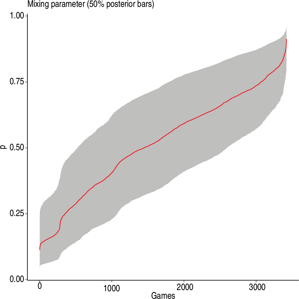
Figure 3 displays the ordered 50% credible bars for the marginal posteriors of the mixing parameter $p_{m}, m = 1, \dots, M$ , which appears in (3.3), computed for the EPL. This plot suggests that the amount of information that stems from the bookmakers is comparable with that arising from historical information. Then, the convex combination in (3.3) seems to be an adequate option for our purposes. Plotting 95% intervals would have been less useful, since we would have had overly great bars for a parameter which is constrained between 0 and 1.

Figure 2:

Posterior 50% credible bars for the attack (red) and the defence (blue) effects along the 10 seasons for the teams belonging to the EPL 2016–2017. Wider posterior bars are associated with teams reporting fewer observations

4.3 Model fit

As broadly explained in Gelman et al. (2014), once we obtain some estimates from a Bayesian model we should assess the fit of this model to the data at hand and the plausibility of such model, given the purposes for which it was built. The principal tool designed for achieving this task is ‘posterior predictive checking’. This post-model procedure consists of verifying whether some additional replicated data under our model are consistent with the observed data. Thus, we draw simulated values $y^{rep}$ from the joint predictive distribution of replicated data:

p (y^{rep} | y) = \int_{Θ} p (y^{rep}, θ | y) d θ = \int_{Θ} p (θ | y) p (y^{rep} | θ) d θ .

(4.1)

It is worth noting that the symbol

y^{rep}

used here is different from the symbol

\tilde{y}

used in the next section. The former is just a replication of

y

, the latter is any future observable value.

Then, we define a test statistic $T (y)$ for assessing the discrepancy between the model and the data. A lack of fit of the model with respect to the posterior predictive distribution may be measured by tail-area posterior probabilities, or Bayesian $p$ -values

p_{B} = P (T (y^{rep}) > T (y) | y) .

(4.2)

As a practical utility, we usually do not compute the integral in (4.1), but compute the posterior predictive distribution through simulation. If we denote with

θ^{(h)}, h = 1, \dots, H

the

h

th MCMC draw from the posterior distribution of

θ

, we just draw

y^{rep}

from the predictive distribution

p (y^{rep} | θ^{(h)})

. Hence, an estimate for the Bayesian

p

-value is given by the proportion of the

H

simulations for which the quantity

T (y^{rep (h)})

exceeds the observed quantity

T (y)

. From an interpretative point of view, an extreme

p

-value—too close to 0 or 1—suggests a lack of fit of the model compared to the observed data.

Rather than comparing the posterior distribution of some statistics with their observed values (Gelman et al., 2014), we propose a slightly different approach, allowing for a broader comparison of the replicated data under the model. Figure 4 (Panel (a)) displays the replicated distributions $y_{1}^{rep} - y_{2}^{rep}$ (grey areas) conditioned on a given observed goal difference (denoted with blue horizontal lines) from the EPL. From this plot the fit of the model seems good: in other words, the replicated data under the model are plausible and close to the data at hand. As may be noted, our model slightly overestimates the conditional draw probability: apparently, there is no need to furtherly model the so called ‘draw inflation’ issue (Karlis and Ntzoufras, 2003, 2009). Moreover, the variability of the replicated goal difference amounting to $-$ 1, 0, 1 is greater than the variability for a goal difference of $-$ 3 or 3. Apart from the draws, the observed goal differences always fall within the replicated distributions.

Figure 4 (Panel (b)) displays the 50% and 95% credible uncertainty intervals (dark yellow and yellow, respectively) for the ordered estimated goal differences. Blue points are the observed goal differences. About 95.1% of the observed points fall within the 95% uncertainty intervals, and this suggests a good model calibration.

Figure 3:

Ordered posterior 50% credible bars for mixing parameter p for EPL (from 2007–2008 to 2015–2016), 3420 matches

Overall measure of goodness of fit

In Bayesian statistics, it is usual to compare competing models through some criteria based on trade-off between the fit of the data to the model and the corresponding complexity of the model (Spiegelhalter et al., 2002), such as deviance information criterion (DIC). Denoted with $D (θ) = - 2 \log L (θ; y)$ the deviance for a generic model with data $y$ , parameter(s) $θ$ and likelihood $L$ , the posterior mean deviance is $\bar{D} = E_{θ | y} [D (θ)]$ , while the ‘effective number of parameters’ is $p_{D} = \bar{D} - D (E_{θ | y} [θ])$ . Then, DIC is defined as a sum between a ‘goodness of fit’ measure and a ‘complexity’ measure:

DIC = \bar{D} + p_{D} .

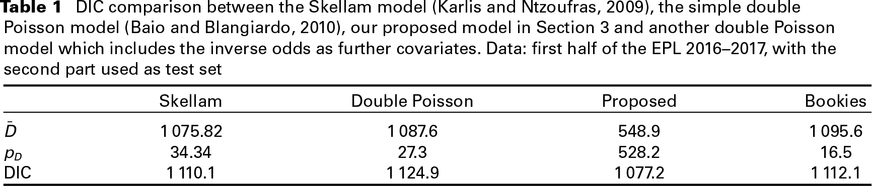
The lower is the DIC, and the better is the model supported by the data. Of course, DIC may be negative as well. Table 1 shows the posterior mean deviance, the effective number of parameters and DIC for four competing models, considering the EPL 2016–2017. For the sake of brevity, we do not report here the results for the other leagues, which are quite similar to those obtained for the EPL. Still, according to a simpler DIC interpretation, we focused here on the 2016–2017 season only; in fact, considering more seasons, as we did in the previous sections, just yields an increase of the model complexity, but mirrors the same DIC pattern observed for one season only. The four models considered are: the Skellam model (Karlis and Ntzoufras, 2009), a simple double Poisson model (Baio and Blangiardo (2010)), our proposed model and a further model (marked with the term Bookies) which includes the bookies inverse odds as model covariates in the scoring rates in the following way:

\begin{matrix} \begin{matrix} \log (θ_{m 1}) & = μ + home + {att}_{t [m] 1} + {def}_{t [m] 2} + \frac{α}{2} o_{Win} + β o_{Draw} - \frac{γ}{2} o_{Loss} \\ \log (θ_{m 2}) & = μ + {att}_{t [m] 2} + {def}_{t [m] 1} - \frac{α}{2} o_{Win} + β o_{Draw} + \frac{γ}{2} o_{Loss} . \end{matrix} \end{matrix}

(4.3)

As it is evident, our model yields the lowest DIC (1077.2) and the lowest $\bar{D}$ (548.9)—proposed by some authors as an alternative measure of fit, due to its robustness and invariance to the parametrization. The complexity of our model is huge if compared with the other models, due to the odds inclusion. As a very rough rule of thumb, DIC's differences of more than 10 should definitely favour the model with the lowest DIC in place of the model with the highest DIC, and this is the case.

Table 1:

DIC comparison between the Skellam model (Karlis and Ntzoufras, 2009), the simple double Poisson model (Baio and Blangiardo (2010)), our proposed model in Section 3 and another double Poisson model which includes the inverse odds as further covariates. Data: first half of the EPL 2016–2017, with the second part used as test set

	Skellam	Double Poisson	Proposed	Bookies
$\bar{D}$	1 075.82	1 087.6	548.9	1 095.6
$p_{D}$	34.34	27.3	528.2	16.5
DIC	1 110.1	1 124.9	1 077.2	1 112.1

4.4 Model assumptions

In this section, we quickly assess whether the main assumptions for our proposed model hold. The strategy is to use posterior predictive tools for detecting possible conflicts between the model and the data. But the diagnostic measures developed here may also act as a sort of inverse tool, revealing that replicated data exhibit some unexpected features.

Conditional independence

Considering $y_{m 1} | θ_{m 1}, λ_{m 1}$ and $y_{m 2} | θ_{m 2}, λ_{m 2}$ as independent implies that the home scores and the away scores are conditionally uncorrelated. Conversely, conditionally correlated scores imply an amount of conditional dependence. Figure 5 displays the distribution of three MCMC correlation coefficients (Pearson $ρ$ , Kendall $τ$ and Spearman $ρ_{s}$ ) along with the observed correlation for the marginal distributions of $y_{m 1}$ and $y_{m 2}$ . As may be noted for each of the three correlation coefficients, the support of the empirical distribution is $ℝ^{+}$ , meaning that there is a suggestion of positive conditional correlation, and, then, of positive conditional dependence. Marginal observed correlation is about zero. Even without specifying a parametric dependence, the MCMC model replications behave as if this dependence had been assumed.

Figure 4:

PP checks for the goal difference $y_{1} - y_{2}$ in EPL against the replicated goal difference $y_{1}^{rep} - y_{2}^{rep}$ . Panel (a): goal differences distribution (grey areas) conditioned on the observed probability (blue segments). Panel (b): 95% posterior intervals (light yellow) and 50% posterior intervals (dark yellow) for estimated goal difference $y_{1}^{rep} - y_{2}^{rep}$ . Blue points are the ordered observed goal differences

Draw inflation

As already mentioned, predicting less draws than the actual ones is a well-known problem in modelling football outcomes. Poisson based models may suffer from this underestimation, and for this reason Karlis and Ntzoufras (2009) propose a zero inflated model for favouring the draw outcome. Nonetheless, this is not the case for our proposed model, which actually overestimates the number of draws, as suggested by Figure 4 (Panel (a)).

Overdispersion

As it is well known, Poisson based models do not allow for overdispersion. In many cases, the variance for a discrete set of data may be greater than its mean, and the Poisson distribution is not well suited in such situations. As broadly documented in the supplementary material, we found that replicated variances are greater than the replicated means; analogously as the interpretation for the conditional dependence, MCMC replications suggest there is no need for explicitly modelling the marginal overdispersion.

4.5 Prediction and posterior probabilities

The main appeal of a statistical model relies on its predictive accuracy. As usual in a Bayesian framework, the prediction for a new dataset may be performed directly via the posterior predictive distribution for our unknown set of observable values. Following the same notation of Gelman et al. (2014), let us denote with $\tilde{y}$ a generic unknown observable. Its distribution is then conditional on the observed $y$ ,

p (\tilde{y} | y) = \int_{Θ} p (\tilde{y}, θ | y) d θ = \int_{Θ} p (θ | y) p (\tilde{y} | θ) d θ,

(4.4)

where the conditional independence of $y$ and $\tilde{y}$ given $θ$ is assumed. As mentioned before, we do not work out a close form for this distribution, but we obtain it via simulation. Thus, every probabilistic computation in this section relies on the following replication experiment: we simulated the 380 matches for the 2016–2017 season according to our model and the posterior estimates based on the previous nine seasons. Collecting the results for each simulated game at each MCMC iteration, we can take advantage of the whole results distribution, and build tools such as the predicted final rank, or the estimated posterior probabilities for each position.

Figure 6 displays the posterior predictive distributions for the following matches: Eintracht Frankfurt-RB Leipzig, German Bundesliga 2016–2017; Hull-Middlesbrough, EPL 2016–2017; Real Madrid-Barcelona, Spanish La Liga 2016–2017; Sampdoria-Juventus, Italian Serie A 2016–2017. The red squares indicate the observed results. Darker regions are associated with higher posterior probabilities. According to the model, the most likely result for the first and the second game is (0,0), with an associated posterior probability about 0.1 and 0.15, respectively, where as the most likely result coincides with the actual result (0,1) for the fourth game. These plots provide a picture that acknowledges the large uncertainty of the prediction. We would not be much interested in a model that often indicates a rare result that has been observed as the most likely outcome; the outcome (2,3) in Real Madrid-Barcelona had a low probability to arise, and a model which would suggest such an outcome as more likely than (1,1) or (1,0) could suffer from some predictive inefficiency. Thus, being aware of the unpredictable nature of football, we would like to grasp the posterior uncertainty of a match outcome in such a way that the actual result is not extreme in the predictive distribution.

Figure 5:

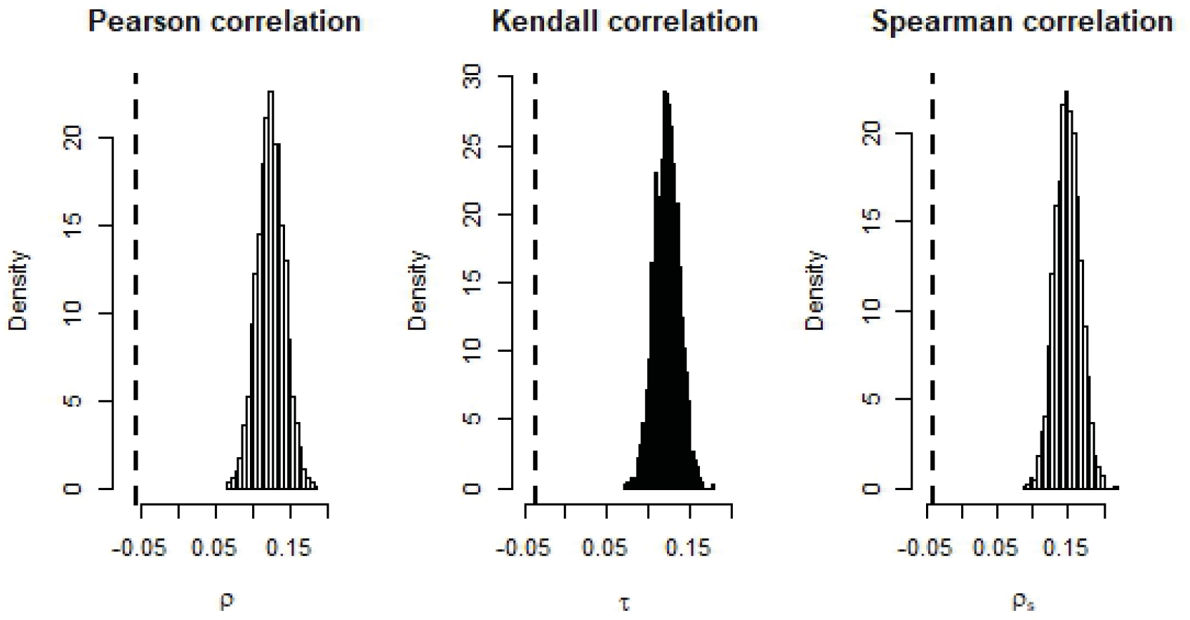
MCMC distribution for the Pearson correlation coefficient $ρ$ , the Kendall correlation coefficient $τ$ and the Spearman correlation coefficient $ρ_{s}$ between the replicated scores $y_{m 1}^{rep}$ and $y_{m 1}^{rep}$ for $m = 1, \dots, M$ for the EPL. The dashed black line denotes the observed correlations between the marginal distributions of the observed scores $y_{m 1}, y_{m 2}$

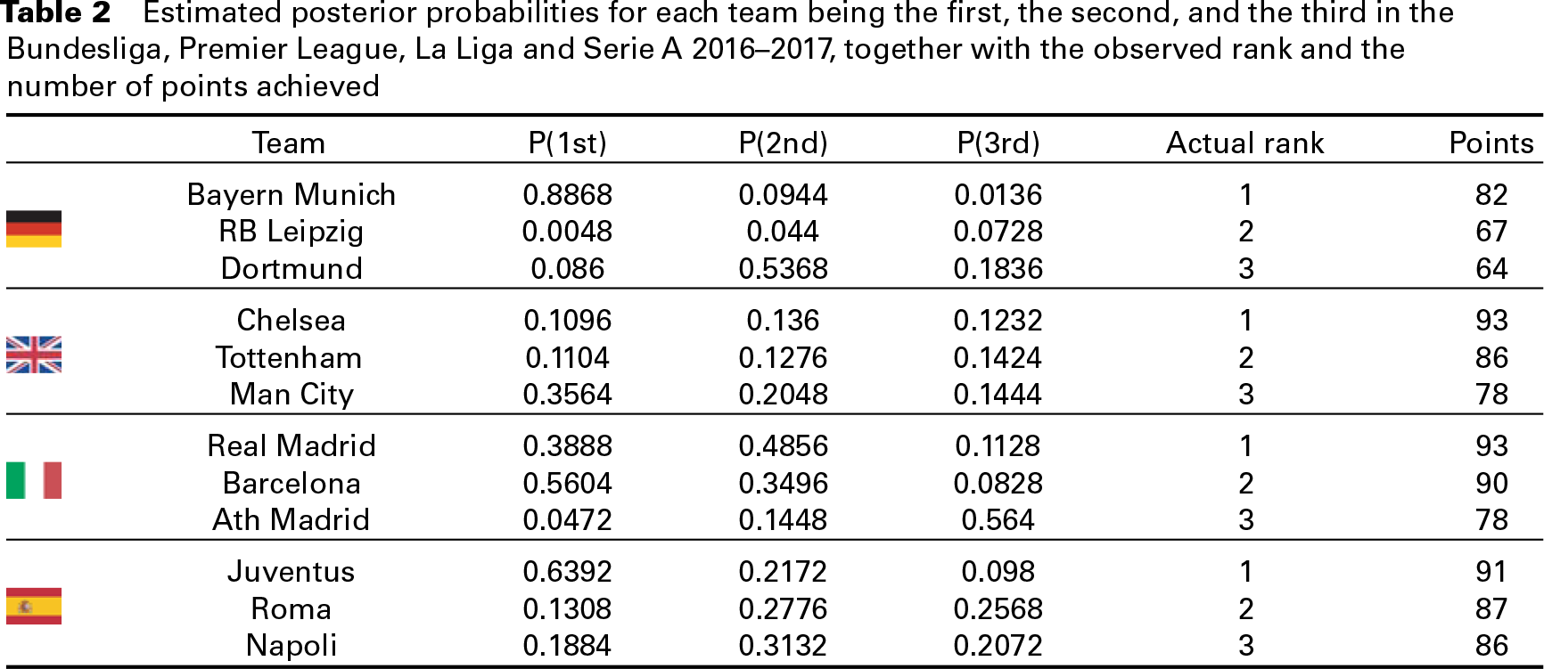
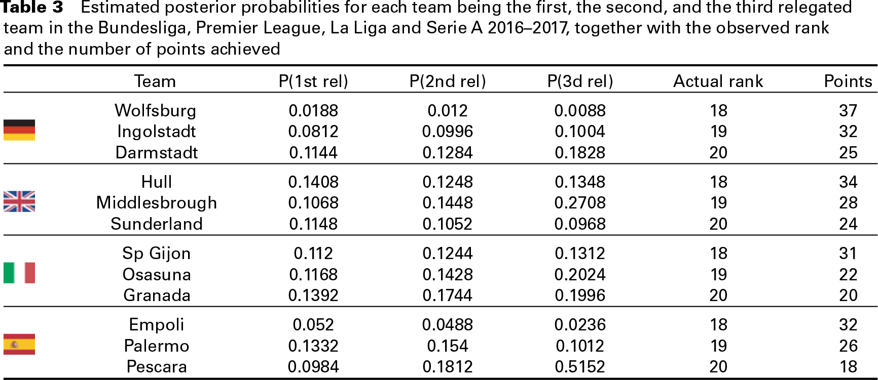
Tables 2 and 3 report the estimated posterior probabilities for each team being the first, the second, and the third; the first relegated, the second relegated, and the third relegated for each of the top four leagues, together with the observed rank and the achieved points, respectively. According to the fit of the previous seasons, Bayern Munich has an estimated probability 0.89 of winning the German league in 2016–2017, which it actually did; in Italy, Juventus has an high probability of being the first (0.64) as well. Conversely, Chelsea has a low associated probability to win the EPL (0.11), and this is mainly due to the bad results obtained by Chelsea in the previous season. Of course, the model does not account for the players’/managers’ transfer market occurring in the summer period. In July 2016, Chelsea hired Antonio Conte, one of the best European managers, who won the EPL on his first attempt. For the relegated teams, it is worth noting that Pescara in Serie A has high estimated probability to be the worst team of the Italian league (0.51). Globally, the model appears able to identify the teams with an associated high relegation's posterior probability.

Table 2:

Estimated posterior probabilities for each team being the first, the second, and the third in the Bundesliga, Premier League, La Liga and Serie A 2016–2017, together with the observed rank and the number of points achieved

Team	P(1st)	P(2nd)	P(3rd)	Actual rank	Points
Bayern Munich	0.8868	0.0944	0.0136	1	82
RB Leipzig	0.0048	0.044	0.0728	2	67
Dortmund	0.086	0.5368	0.1836	3	64
Chelsea	0.1096	0.136	0.1232	1	93
Tottenham	0.1104	0.1276	0.1424	2	86
Man City	0.3564	0.2048	0.1444	3	78
Real Madrid	0.3888	0.4856	0.1128	1	93
Barcelona	0.5604	0.3496	0.0828	2	90
Ath Madrid	0.0472	0.1448	0.564	3	78
Juventus	0.6392	0.2172	0.098	1	91
Roma	0.1308	0.2776	0.2568	2	87
Napoli	0.1884	0.3132	0.2072	3	86

Table 3:

Estimated posterior probabilities for each team being the first, the second, and the third relegated team in the Bundesliga, Premier League, La Liga and Serie A 2016–2017, together with the observed rank and the number of points achieved

Team	P(1st rel)	P(2nd rel)	P(3d rel)	Actual rank	Points
Wolfsburg	0.0188	0.012	0.0088	18	37
Ingolstadt	0.0812	0.0996	0.1004	19	32
Darmstadt	0.1144	0.1284	0.1828	20	25
Hull	0.1408	0.1248	0.1348	18	34
Middlesbrough	0.1068	0.1448	0.2708	19	28
Sunderland	0.1148	0.1052	0.0968	20	24
Sp Gijon	0.112	0.1244	0.1312	18	31
Osasuna	0.1168	0.1428	0.2024	19	22
Granada	0.1392	0.1744	0.1996	20	20
Empoli	0.052	0.0488	0.0236	18	32
Palermo	0.1332	0.154	0.1012	19	26
Pescara	0.0984	0.1812	0.5152	20	18

Figure 6:

Posterior predictive distribution of the possible results for the following matches: Eintracht Frankfurt-RB Leipzig, German Bundesliga 2016–2017; Hull-Middlesbrough, English Premier League 2016–2017; Real Madrid-Barcelona, Spanish La Liga 2016–2017; Sampdoria-Juventus, Italian Serie A 2016–2017. All the plots report the posterior uncertainty related to the exact predicted outcome. Darker regions are associated with higher posterior probabilities and red square corresponds to the observed result

Figure 7 provides posterior 50% credible bars (grey ribbons) for the predicted achieved points for each team in top four European leagues 2016–2017 at the end of their respective seasons, together with the observed final ranks. Displaying 50% credible bars results to be cleaner than 95% bars, and highlights the predictive power of the model in terms of 50% out-of-sample calibration. At a first glance, the four predicted posterior ranks appear to detect a pattern similar to the observed ones, with only a few exceptions. As may be noticed for Bundesliga (Panel (a)), Bayern Munich's prediction mirrors its actual strength in the 2016–2017 season, where as RB Leipzig performance was definitely underestimated by the model. Still, the model does not take into consideration the budget of each team, and the fact that RB Leipzig was one of the richest teams in the Bundesliga in 2016–2017. In the EPL (Panel (b)), Chelsea is underestimated by the model, where as Manchester City is the favourite team. The predicted pattern for the Spanish La Liga (Panel (c)) is extremely close to the one we observed, apart from the winner (our model favoured Barcelona, second in the observed rank). The worst teams (Sporting Gijon, Osasuna and Granada) are correctly predicted to be relegated. Also, for the Italian Serie A, the predicted ranks globally match the observed ranks. The outlier is represented by Atalanta, a team that performed incredibly well and qualified for the Europa League at the end of the last season. As a general comment, we may conclude that these plots show a good model calibration, since more or less half of the observed points fall in the posterior 50% credible bars.

5 A preliminary betting strategy

In this section we provide a real betting experiment, assessing the performance of our model compared to the existing betting odds. In a betting strategy, two main questions arise: it is worth betting on a given single match? If so, how much is worth betting? In Section 2, we described two different procedures for inferring a vector of betting probabilities $Π$ from the inverse odds vector O. The common expression ‘beating the bookmakers’ may be interpreted in two distinct ways: from a probabilistic point of view, and from a profitability point of view. According to the first definition, which is more appealing for statisticians, a bookmaker is beaten whenever our matches’ probabilities are more favourable than their probabilities. As before, let $π_{i, m}^{s}$ denote the betting probabilities provided by the $s$ th bookmaker for the $m$ th game, with $i \in Δ_{m} = {' W i n',' D r a w',' L o s s'} .$ Additionally, let $Y_{m 1}$ and $Y_{m 2}$ denote the random variables representing the number of goals scored by two teams in the $m$ th match. From our model in (3.3), we can compute the following three-way model's posterior probabilities: $p_{w i n, m} = P (Y_{m 1} 〉 Y_{m 2} | y), p_{D r a w, m} = P (Y_{m 1} = Y_{m 2} | y), p_{L o s s, m} = P (Y_{m 1} 〈 Y_{m 2} | y)$ for each $m \in Τ_{s},$ conditioned on the past outcomes $y$ , using the results of the Skellam distribution outlined in Section 3. In fact, $Y_{m 1} - Y_{m 2} \sim P D ({\hat{γ}}_{m 1}, {\hat{γ}}_{m 2}),$ where ${\hat{γ}}_{m 1} = {\hat{p}}_{m 1} {\hat{θ}}_{m 1} + (1 - {\hat{p}}_{m 1}) {\hat{λ}}_{m 1} a n d {\hat{γ}}_{m 2} = {\hat{p}}_{m 2} {\hat{θ}}_{m 2} + (1 - {\hat{p}}_{m 2}) {\hat{λ}}_{m 2}$ are the convex combinations of the posterior estimates obtained through the MCMC sampling. Thus, the global average probability of a correct prediction for our model may be defined as:

\bar{p} = \frac{1}{M} \sum_{m = 1}^{M} \prod_{i \in Δ_{m}} {p_{i, m}}^{δ_{im}},

(5.1)

where $δ_{im}$ denotes the Kronecker's delta, with $δ_{im} = 1$ if the observed result at the $m$ th match is $i, i \in Δ_{m}$ . This quantity serves as a global measure of performance for comparing the predictive accuracy between the posterior match probabilities provided by the model and those obtained from the bookies odds.

Table 4:

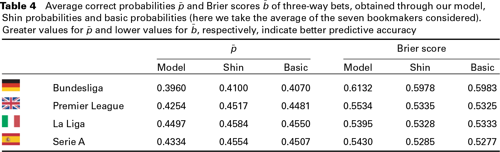
Average correct probabilities $\bar{p}$ and Brier scores $\bar{b}$ of three-way bets, obtained through our model, Shin probabilities and basic probabilities (here we take the average of the seven bookmakers considered). Greater values for $\bar{p}$ and lower values for $\bar{b}$ , respectively, indicate better predictive accuracy

	$\bar{p}$			Brier score
	Model	Shin	Basic	Model	Shin	Basic
Bundesliga	0.3960	0.4100	0.4070	0.6132	0.5978	0.5983
Premier League	0.4254	0.4517	0.4481	0.5534	0.5335	0.5325
La Liga	0.4497	0.4584	0.4550	0.5395	0.5328	0.5333
Serie A	0.4334	0.4554	0.4507	0.5430	0.5285	0.5277

Moreover, we may compute the Brier score (Brier, 1950), another index used for the predictive accuracy and previously used by Spiegelhalter and Ng (2009) for assessing football predictive accuracy:

\bar{b} = \frac{1}{M} \sum_{1 = 1}^{M} \sum_{i = 1}^{3} (p_{i, m} - δ_{i, m})^{2} .

(5.2)

The Brier score is a sort of mean squared error of the forecasts, ranging from 0 to 2. The lower is the Brier core, and the better is the model predictive accuracy. As reported in Table 4, our model is very close to the bookmakers’ probabilities (Shin's method and basic procedure) for what concerns both $\bar{p}$ and $\bar{b}$ . At a first glance, one may be tempted to say that, according to these measures, our model does not improve the bookmakers’ probabilities. However, these indexes are only an average measure of the predictive power, which does not take into account the possible profits for the single matches.

Figure 7:

Posterior 50% credible bars (grey ribbons) for the achieved final points of the top-four European leagues 2016–2017. Black dots are the observed points. Black lines are the posterior medians. At a first glance, the pattern of the predicted ranks appears to match the pattern of the observed ones, and the model calibration appears satisfying

According to the second definition, ‘beating the bookmaker’ means earning money by betting according to our model's probabilities. One could bet one unit on the three–way match outcome with the highest expected return (Strategy A), or place different amounts, basing each bet on the match's profit variability, as suggested in Rue and Salvesen (2000) (Strategy B). Denoted with $j_{m}$ and $w_{m}$ the three-way outcome with the highest expected return and the money invested in the $m$ -th match respectively, the expected profit $X_{m}$ is then defined as:

X_{m} = \frac{p_{j_{m}, m}}{o_{j_{m}, m}} - w_{m} \sum_{i_{m} \neq j_{m}} p_{i_{m}, m} .

The expected profits (percentages divided by 100) for our model and according to the bookmakers’ probabilities are reported in Figure 8 in terms of their mean $\pm$ standard deviations. Gambling with the bookies probabilities, we always have expected losses. Conversely, betting with our posterior model probabilities yields high expected profits for each league and each bookmaker. It is worth noting that positive expected profits do not assure high positive returns, but they provide a tool for assessing the goodness of our model-based strategy over the long run.

6 Discussion and further work

We have proposed a new hierarchical Bayesian Poisson model in which the rates are convex combinations of parameters accounting for two different sources of data: the bookmakers’ betting odds and the historical match results. We transformed the inverse betting odds into probabilities and we worked out the bookmakers’ scoring rates through the Skellam distribution. A wide graphical and numerical analysis for the top four European leagues has shown a good predictive accuracy for our model, and surprising results in terms of expected profits. These results confirm on one hand that the information contained in the betting odds is relevant in terms of football prediction; on the other hand that, combining this information with historical data allows for a natural extension of the existing models for football scores.

Further work should be done in order to include a parametric dependence in the proposed model.

Figure 8:

Distribution of the expected profits (%/100) $X_{m}$ , expressed in terms of mean $\pm$ standard deviations for the seven bookmakers considered, for each of the top four European leagues

Declaration of conflicting interests

The authors declared no potential conflicts of interest with respect to the research, authorship and/or publication of this article.

Funding

The authors received no financial support for the research, authorship and/or publication of this article.

References

Baio

Blangiardo

(2010) Bayesian hierarchical model for the prediction of football results. Journal of Applied Statistics , 37, 253–64.

Brier

(1950) Verification of forecasts expressed in terms of probability. Monthly Weather Review , 78, 1–3.

Cain

Law

Peel

(2002) Is one price en- ough to value a state-contingent asset corr- ectly? Evidence from a gambling market. Applied Financial Economics , 12, 33–8.

Cain

, Law

Peel

(2003) The favourite-longshot bias, bookmaker margins and insider trading in a variety of betting markets. Bulletin of Economic Research , 55, 263–73.

Dixon

Coles

(1997) Modelling association football scores and ineffciencies in the football betting market. Journal of the Royal Statistical Society: Series C (Applied Statistics), 46, 265–80.

Dixon

Robinson

(1998) A birth process model for association football matches. Journal of the Royal Statistical Society: Series D (The Statistician) , 47, 523–38.

Epstein

(1969) A scoring system for probability forecasts of ranked categories. Journal of Applied Meteorology , 8, 985–87.

Forrest

Goddard

Simmons

(2005) Odds-setters as forecasters: The case of English football. International Journal of Forecasting , 21, 551–64.

Forrest

Simmons

(2002) Outcome uncertainty and attendance demand in sport: The case of English soccer. Journal of the Royal Statistical Society: Series D (The Statistician) , 51, 229–41.

10.

Gelman

Carlin

Stern

Rubin

(2014) Bayesian Data Analysis. Vol. 2. Boca Raton, FL: Chapman & Hall/CRC.

11.

Groll

Abedieh

(2013) Spain retains its title and sets a new record-generalized linear mixed models on European football championships. Journal of Quantitative Analysis in Sports , 9, 51–66.

12.

Groll

, Schauberger

Tutz

(2015) Predi- ction of major international soccer tourna- ments based on team-specic regularized Poisson regression: An application to the FIFA World Cup 2014. Journal of Quan- titative Analysis in Sports , 11, 97–115.

13.

Hoeting

Madigan

Raftery

Volinsky

(1999) Bayesian model averaging: A tutorial. Statistical Science , 14, 382–401.

14.

Jullien

Salanie

(1994) Measuring the incidence of insider trading: A comment on Shin. Economic Journal , 104, 1418–19.

15.

Karlis

Ntzoufras

(2003) Analysis of sports data by using bivariate Poisson models. Journal of the Royal Statistical Society: Series D (The Statistician) , 52, 381–93.

16.

Karlis

Ntzoufras

(2009) Bayesian modelling of football outcomes: Using the Skellam's distribution for the goal difference. IMA Journal of Management Mathematics , 20, 133–45.

17.

Koopman

Lit

(2015) A dynamic bivariate Poisson model for analysing and forecasting match results in the English Premier League. Journal of the Royal Statistical Society: Series A (Statistics in Society), 178, 167–86.

18.

Koopman

Lit

(2017) Forecasting football match results in national league competitions using score-driven time series models (Technical report). Amsterdam: Tinbergen Institute.

19.

Londono

Hassan

(2015) Sports betting odds: A source for empirical Bayes (Technical report). Medellín: EAFIT University.

20.

Maher

(1982) Modelling association football scores. Statistica Neerlandica , 36, 109–18.

21.

McHale

Scarf

(2011) Modelling the dependence of goals scored by opposing teams in international soccer matches. Statistical Modelling , 11 (3), 219–236.

22.

Ntzoufras

(2011) Bayesian modeling using WinBUGS. Vol. 698. Hoboken, New Jersey, USA: John Wiley & Sons.

23.

Owen

(2011) Dynamic Bayesian forecasting models of football match outcomes with estimation of the evolution variance para- meter. IMA Journal of Management Mathematics , 22, 99–113.

24.

Plummer

(2017) Jags version 4.3.0 user manual . URL sourceforge. net/projects/mcmc-jags/es/ Manuals/4.x (last accessed 29 August 2018).

25.

Rue

Salvesen

(2000) Prediction and retrospective analysis of soccer matches in a league. Journal of the Royal Statistical Society: Series D (The Statistician), 49, 399–418.

26.

Shin

(1991) Optimal betting odds against insider traders. The Economic Journal , 101, 1179–85.

27.

Shin

HSa

(1993) Measuring the incidence of insider trading in a market for state-contingent claims. The Economic Journal , 103, 1141–53.

28.

Smith

Paton

Williams

(2009) Do bookmakers possess superior skills to bettors in predicting outcomes? Journal of Economic Behavior & Organization , 71, 539–49.

29.

Spiegelhalter

Y-L

(2009) One match to go! Significance, 6, 151–53.

30.

Spiegelhalter

Best

Carlin

Van

Der

Linde

(2002) Bayesian measures of model complexity and fit. Journal of the Royal Statistical Society: Series B (Statistical Methodology) , 64, 583–639.

31.

Štrumbelj

(2014) On determining probability forecasts from betting odds. International Journal of Forecasting , 30, 934–43.

Combining historical data and bookmakers’ odds in modelling football scores

Abstract

Keywords

1 Introduction

2 Transforming the betting odds into probabilities

3.1 Model for the scores

4.1 Data

4.2 Parameter estimates

Figure 2:

Posterior 50% credible bars for the attack (red) and the defence (blue) effects along the 10 seasons for the teams belonging to the EPL 2016–2017. Wider posterior bars are associated with teams reporting fewer observations

Ordered posterior 50% credible bars for mixing parameter p for EPL (from 2007–2008 to 2015–2016), 3420 matches

Overall measure of goodness of fit

Conditional independence

Figure 4:

Draw inflation

Overdispersion

Estimated posterior probabilities for each team being the first, the second, and the third in the Bundesliga, Premier League, La Liga and Serie A 2016–2017, together with the observed rank and the number of points achieved

Estimated posterior probabilities for each team being the first, the second, and the third relegated team in the Bundesliga, Premier League, La Liga and Serie A 2016–2017, together with the observed rank and the number of points achieved

Distribution of the expected profits (%/100) X m , expressed in terms of mean ± standard deviations for the seven bookmakers considered, for each of the top four European leagues

Declaration of conflicting interests

Funding

References

Distribution of the expected profits (%/100) $X_{m}$ , expressed in terms of mean $\pm$ standard deviations for the seven bookmakers considered, for each of the top four European leagues