
Abstract
Multiple responses of mixed types are naturally encountered in a variety of data analysis problems, which should be jointly analysed to achieve higher efficiency gains. As an efficient approach for joint modelling, the latent variable model induces dependence among the mixed outcomes through a shared latent variable. Generally, the latent variable is assumed to be normal, which is not that flexible and realistic in practice. This tutorial article demonstrates how to jointly analyse mixed continuous and ordinal responses using a semiparametric latent variable model by allowing the latent variable to follow a Dirichlet process (DP) prior, and illustrates how to implement Bayesian inference through a powerful R package nimble. Two model comparison criteria, deviance information criterion (DIC) and logarithm of the pseudo-marginal likelihood (LPML), are employed for model selection. Simulated data and data from a social survey study are used for illustrating the proposed method with nimble. An extension of DP prior to DP mixtures prior is introduced as well.
Introduction
Multivariate responses of mixed data types are common in a variety of data analysis contexts, like multiple aspects of a topic that is of interest in survey sampling. In order to take account of the relationships among multiple responses, joint modelling is more preferred than separate analysis due to significant efficiency gains (McCulloch, 2008). In joint modelling analysis, the key is to build a joint distribution for multivariate responses. However, it is not straightforward to build a joint distribution for responses of mixed data types. One approach is employing copulas to model the joint distribution, which is relatively difficult to implement (Song and Song, 2007). Factorizing the joint distribution of the multivariate responses is another approach, for example, specifying the joint distribution of mixed continuous and discrete responses as a product of a marginal distribution of one set of responses and a conditional distribution of another set of responses. This approach is easy to understand and implement, but the main drawback is that different directions of factorization may lead to different results (Wu, 2013). The latent variable model (LVM), also referred as generalized latent trait model in Sammel et al. (1997) and Moustaki and Knott (2000), is another useful tool for joint modelling mixed responses, which is relatively straightforward and easy to implement. In LVM, a shared latent variable is set up to induce dependence among mixed continuous and discrete outcomes. Based on an assumption that the outcomes are conditionally independent given this latent variable, a joint model of these mixed outcomes can be built. For parameter estimation of LVM, both expectation–maximization (EM) algorithm and the Bayesian approach are used in the literature. In this article, we employ the Bayesian approach for inference due to its flexibility.
Generally, the latent variable in LVM is assumed to follow a normal distribution. However, this assumption may not be always true in practice. In order to overcome the limitation of the normality assumption, robust methods have been proposed in the literature, including multivariate t-distribution, skew-normal distribution and nonparametric priors. Multivariate t-distribution is usually used for non-normal data with symmetrical heavy tails (Shapiro and Browne, 1987; Kano et al., 1993; Lee and Xia, 2006). The skew-normal distribution is able to model skewed and non-symmetric continuous responses through a parametric distribution (Azzalini, 1985; Azzalini and Capitanio, 1999; Lin et al., 2009; Baghfalaki and Ganjali, 2011; Lu and Huang, 2014; Teimourian et al., 2015). These methods are both parametric and not flexible enough compared to nonparametric methods. In the Bayesian framework, nonparametric priors provide a flexible approach to address the uncertainty of distributions; see Müller et al. (2015) for a review. Practically, the Dirichlet process (DP) prior is a widely used nonparametric prior in Bayesian analysis; see for example, Ferguson (1973), Antoniak (1974), Escobar (1994), MacEachern and Müller (1998) and among others. In order to allow for direct inferences on the posterior distributions for more general functions, Ishwaran and Zarepour (2000) proposed a truncated version of DP, while Ishwaran and Zarepour (2001) introduced a stick-breaking representation and blocked Gibbs sampler for Bayesian inference to achieve practical and computational convenience. Some applications of DP prior are given by Lee et al. (2008), Gill and Casella (2009), Hwang and Pennell (2014) and Xia and Gou (2016).
In this tutorial article, we consider LVM for mixed continuous and ordinal responses to fit data from Chinese General Society Survey (CGSS) 2013. In order to violate the normality assumption of the latent variable, a DP prior is assigned. Bayesian inference of this semiparametric LVM with an implementation of a finite-dimensional approximation of the DP prior is carried out in nimble. In practice, Bayesian inference is always implemented in softwares and packages including WinBUGS (Spiegelhalter et al., 2003), JAGS (Plummer, 2003) and Stan (Team, 2017). WinBUGS is quite powerful and can handle various types of problems, but convergence of Markov chains would be slow with large and hierarchical structured datasets. JAGS, similar to WinBUGS, is an open-source implementation of BUGS model specification and can be interfaced with R. Stan is another open-source software with functionality similar to WinBUGS, but uses a more complicated Markov chain Monte Carlo (MCMC) algorithm, which allows to converge quickly under complex model settings (Ma and Chen, 2018). However, it is not straightforward to deal with discrete variables in Stan. Considering the complexity of our problem, we use a relatively new and powerful R package nimble (de Valpine et al., 2017) for Bayesian inference. Nimble is an R package for programming with BUGS models using syntax similar to WinBUGS and JAGS, but with more flexibility in defining the models and algorithms. Users can operate from within R, and nimble will generate the C++ code for faster computation.
The aim of this tutorial article is to introduce how to jointly analyse mixed continuous and ordinal responses using a Bayesian semiparametric latent variable model by allowing the shared latent variable to follow a DP prior, as well as its implementation in a relatively new and powerful R package nimble. Data from CGSS 2013 is used for illustration. The proposed semiparmetric LVM is introduced in Section 2. The procedures of Bayesian inference and model selection are provided in Section 3. In Section 4 and Section 5, a simulation study and an empirical analysis are carried out, respectively, to illustrate the proposed methods in nimble. An extension of DP prior to DP mixtures prior is introduced additionally in Section 6. Finally, conclusions and discussions are given in Section 7.
Model specification
Consider a dataset with N subjects and K outcome variables, such that the first K1 outcome variables are continuous, while the remaining
Let L denote the shared latent variable in the LVM, and assume that all the mixed outcomes are conditionally independent given this latent variable. The joint distribution of these mixed continuous and ordinal outcomes is given by

where
For the continuous outcome variable


where
For the ordinal outcome variable ZK, an ordered probit distribution is assigned. The ordinal outcome variable is on a scale of
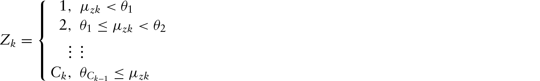
The


where
In classic LVMs, the latent variable L is generally assumed to follow a normal distribution. However, this normality assumption may not be always true in practice. In order to overcome the limitation of the normality assumption of L, a semiparametric approach assigning a DP (Ferguson, 1973) prior for L is considered. Suppose that the latent variable L conforms to an unknown distribution such that

where the concentration parameter κ represents the weight of the base distribution. For realization, DP can be written as an infinite mixture of point masses, and Sethuraman (1994) made this precisely by providing a constructive definition of DP called the stick-breaking construction. It is simply given as

where

where

The weight parameter
Bayesian inference
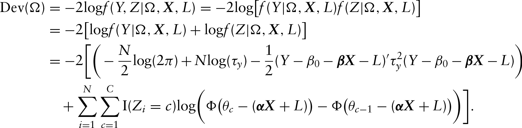
Suppose Ω denotes the unknown parameter vector and

where
The response model described in Section 2 can be written as follows:

where

For

For

In order to obtain the posterior distributions, full conditional distributions of these parameters should be derived first. Generally, Bayesian posterior samples can be obtained from the respective full conditional distributions through MCMC algorithms, which can be implemented in specific software packages such as WinBUGS and JAGS. In this article, we utilize an R package ‘nimble’ for estimation and simply compare it with another common software JAGS to discover the differences in efficiency.
In order to obtain reliable posterior estimations from MCMC samples, it is necessary to monitor and assess the convergence behaviour of the Markov chains. Only samples obtained after the Markov chains converge to the respective stationary distributions can be kept for posterior estimation. Either graphical visualization or certain summary statistics can be applied to monitor the convergence. For convergence diagnostics, Gelman and Rubin's convergence diagnostic (Gelman and Rubin, 1992) is a general measure that can be computed from multiple Markov chains. However, in complex models and large datasets, it is time-consuming to run multiple chains, so graphical visualization is an alternative to assess the convergence. Trace plots and plots of autocorrelation functions (ACFs) are two important tools. When the sampling path in the trace plot of a Markov chain does not show any indication of a trend and autocorrelations are low in ACF plot, the Markov chain can be indicated as well converged.
Model selection
Model selection is an important topic in statistical modelling since the true model is actually unknown. Here we employ two commonly used criteria, DIC and LPML, for model comparison. DIC is defined as

where
Another criterion is LPML, which is obtained based on the conditional predictive ordinate (CPO). Similarly, we calculate the CPO and LPML based on the conditional likelihood. Let

where


Models with a smaller value of DIC is preferred, while models with a larger value of LPML is better.
Simulation study and implementation with nimble
Simulation study
In this section, a simulation study is carried out to illustrate the performance of the model selection criteria and the posterior estimates of the proposed model. For the performance of DIC and LPML, we compare models with different priors on the latent variable and calculate the percentage that the criteria choose the correct model. For the empirical performance of the posterior estimates, bias, the root mean square error (RMSE) and the coverage probability (CP) are employed. Suppose

where t is the number of replications in the simulation. In our simulation, t was set to be 70. CP represents the probability that the 95% credible interval contains the true value of the parameters.
Simulation 1: L is bimodal
Here we assume that the non-normal latent variable L was generated from a mixture of two normal distributions
In order to reveal the performance of DIC and LPML in model selection, we fitted the simulated datasets with the following different priors on the latent variable L:
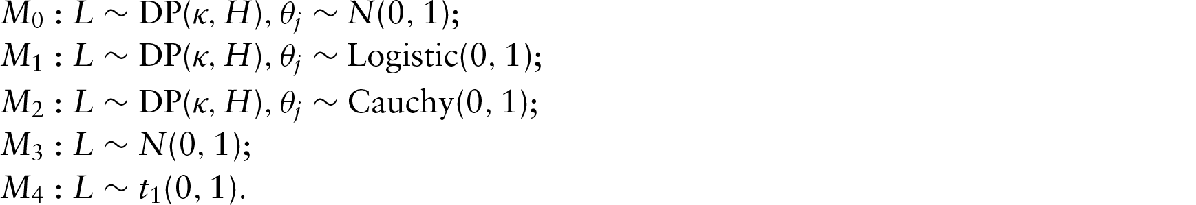
R package nimble were used for programming and estimation. A total of 100 000 iterations were carried out and the thinning interval was set to be 10. The first 500 iterations were discarded as the burn-in phase, while the remaining 9 500 samples were saved for posterior estimation. Due to the computational burden, we ran a single Markov chain and used trace plots and ACF plots for convergence assessment.
Average DIC and LPML values for the five models, M0–M4, are shown in Table 1.
Average DIC and LPML for the competing models when L is bimodal

Average DIC and LPML for the competing models when L is bimodal
From Table 1, we can see that for model M1 with a DP prior on L and a logistic distribution as the base distribution, the DIC value is the smallest and the LPML value is the largest among these alternative models. These two model selection criteria choose M1 as the best model. By comparing the results of the first three models that used a DP prior on L, we can see that the DIC and LPML values are similar, especially for models M1 and M2. For models M3 and M4, their DIC values are much larger than those of the other models, especially for models with the latent variable that follows a normal distribution.
We also calculated the percentages that DIC and LPML chose the best model in the simulation. The percentage of DIC for choosing the best model M1 is 71.43, and the percentage of DIC for not choosing the models M3 and M4 is 100. For LPML, the percentages for choosing M1 and not choosing M3 and M4 are 67.43 and 100, respectively. These values indicate that DIC and LPML perform well in selecting the correct model. The results in Table 1 indicate that when the latent variable is actually non-normal and bimodal, the DP prior performs well and is a good choice in practice.
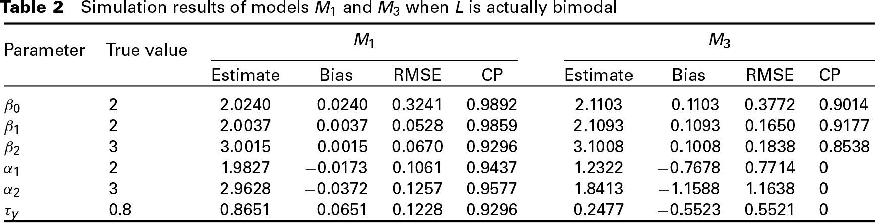
The Bayesian estimates, bias, RMSE and CP of the parameters in the chosen model M1 are shown in Table 2. We can see that the bias and RMSE in M1 are relatively small and both the CPs are larger than 0.92. In Table 2, the results of model M3 with a normal prior on L are shown as well. By comparing the results of M1 and M3, we can see that bias and RMSE in M3 are larger than those in M1, and the CPs are smaller than those in M1, indicating that model with a normal latent variable performs worse than model with a latent variable that follows a DP prior when the latent variable is actually bimodal. These results also conform to the model selection results.
Simulation results of models M1 and M3 when L is actually bimodal
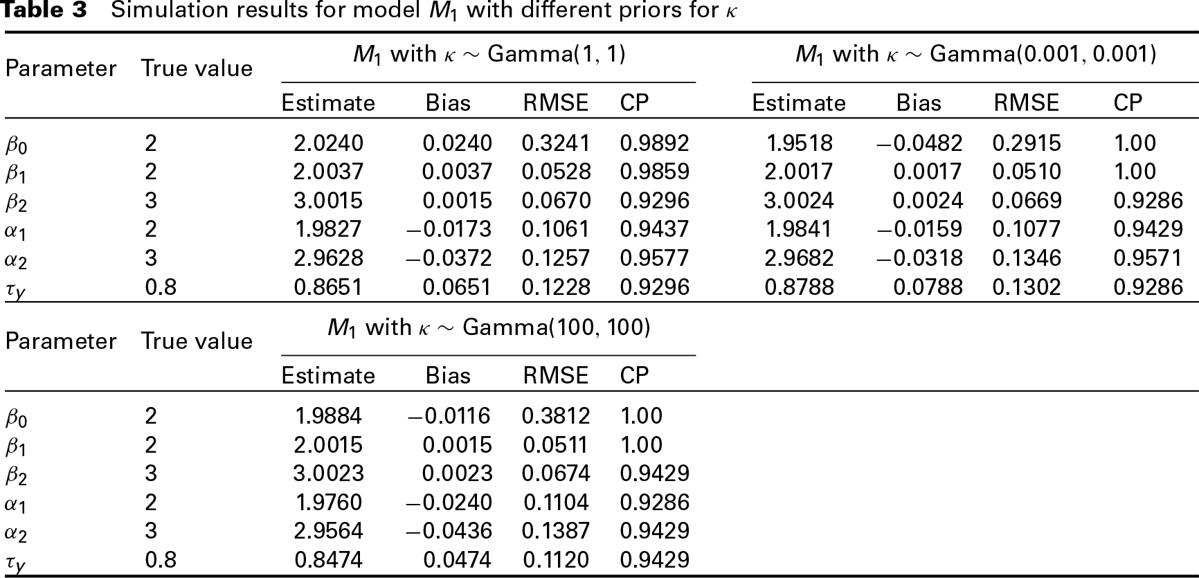
In our model settings, we used an informative hyperprior Gamma(1, 1) for the precision parameter κ in DP prior. Here we perform a sensitivity analysis to study the effect of hyperpriors on κ. We built model M1 with the other two different hyperpriors on κ: Gamma(0.001,0.001) and Gamma(100,100). The simulation results of these three models are shown in Table 3. From Table 3, we can see that the performance of posterior estimates do not change a lot with different hyperpriors on the precision parameter κ, indicating that the model is robust with different hyperpriors on the concentration parameter in DP prior.
Simulation results for model M1 with different priors for κ
We also ran model M1 and conducted Bayesian analysis using JAGS to compare the efficiency of these two tools. Carrying out 100 000 iterations with a thinning interval of 10 for a sample of
In this section, the simulation settings were identical with Simulation 1, except for the true distribution of the latent variable. Here we assume that the non-normal latent variable L was drawn from
Average DIC and LPML for the competing models when L is skewed

Average DIC and LPML for the competing models when L is skewed
From Table 4, we can see that for model M2, the DIC value is the smallest and the LPML value is the largest among these alternative models. These two model selection criteria chose M2 as the best model. Similarly, the DIC and LPML values of the models with L following a DP prior are similar, especially for M1 and M2. For models M3 and M4, their DIC values are much larger than those of the other models, while their LPML values are smaller compared to the other models.
The percentage of DIC for choosing the best model M2 is 73.19, and the percentage for not choosing the model M3 and M4 is 100. For LPML, the percentages for choosing M2 and not choosing M3 and M4 are 70.27 and 100, respectively. These values indicate that DIC and LPML perform well in selecting the correct model under our simulation settings. The results in Table 4 indicate that when the latent variable is actually non-normal and skewed distributed, DP prior performs well and is a good choice in practice.
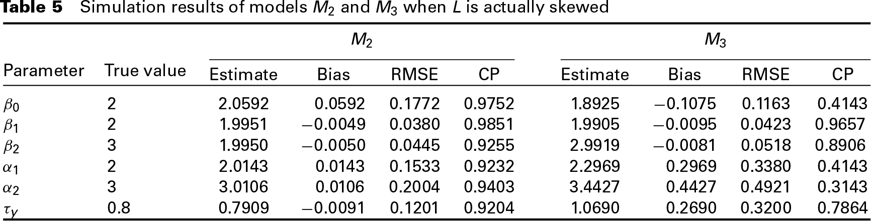
The posterior estimates, bias, RMSE and CP of the parameters in the chosen model M2 are given in Table 5. We can see that the bias and RMSE in M2 are relatively small and both the CPs are larger than 0.92. In Table 5, the simulation results of model M3 are shown as well. Compared to M2, the bias and RMSE in M3 are larger, while the CPs are smaller. These results also conform to the model selection results.
Simulation results of models M2 and M3 when L is actually skewed
In this simulation, the true distribution of the latent variable L was assumed to be the standard normal distribution
Average DIC and LPML for the competing models when L is normal

Average DIC and LPML for the competing models when L is normal
From Table 6 we can see that when L is actually normal, model M3 has the smallest DIC and the largest LPML values among these five models. The results indicate that DIC and LPML choose M3 as the best model, which conforms to the fact that L actually follows a normal distribution. For models with DP priors on the latent variable, model M1 with the logistic base function performs better than the other two models M0 and M2 on both the DIC and LPML values. The percentage of DIC for choosing the best model M3 is 75.71, while the percentage of LPML for choosing M3 is 74.29. These results show that DIC and LPML perform well in selecting the correct model when L actually follows a normal distribution.
The posterior estimates, bias, RMSE and CP of the parameters in the chosen model M3 are given in Table 7. The results of model M1 with a DP prior are shown as well for comparison.
Simulation results of model M3 and M1 when L is actually normal
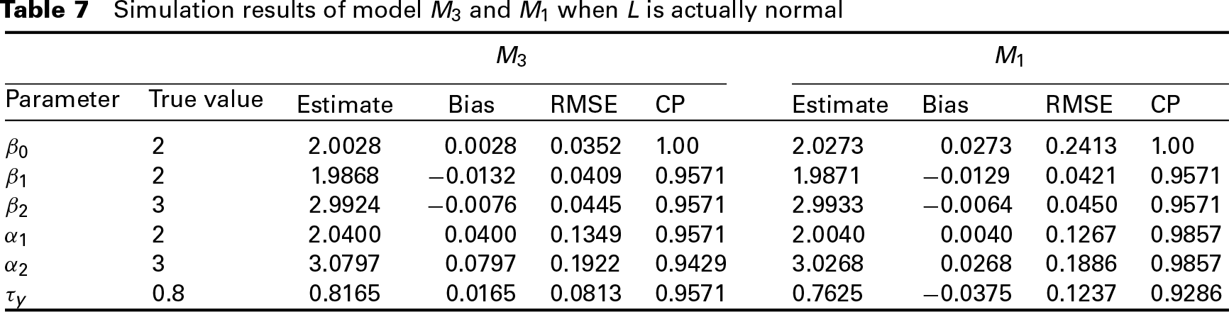
From Table 7 we can observe that when L is actually normally distributed, the posterior estimates in M3 are of small bias and RMSE. However, model M1 with a DP prior for L also behaves well on posterior estimation and the results are close to those in M3. These results indicate that even when L actually follows a normal distribution, a model with a DP prior on the latent variable also performs well and can obtain relatively precise estimation for the parameters.
The proposed semiparametric LVM and Bayesian inference were implemented via nimble. nimble is an R package for programming with BUGS models, which allows for fitting models specified using syntax similar to WinBUGS and JAGS, but with more flexibility in defining the models and algorithms. Users can operate from within R, and nimble will generate the C++ code for faster computation. In this section, we introduce how to carry out the proposed analysis using nimble 0.6–10 in R 3.4.1.
The first step is to create the proposed semiparametric LVM, which includes four parts: model code, constants, data and initial values for MCMC. The syntax of the model code is similar to the BUGS language, which is attractive for users who have coding experiences of WinBUGS and JAGS. The beginning lines for the model code are
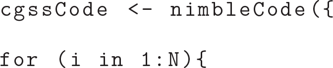
The function nimbleCode() states the code for the model. We loop through 1 to the sample size N for the mixed responses and the latent variable. For the continuous response

where
For the ordinal response
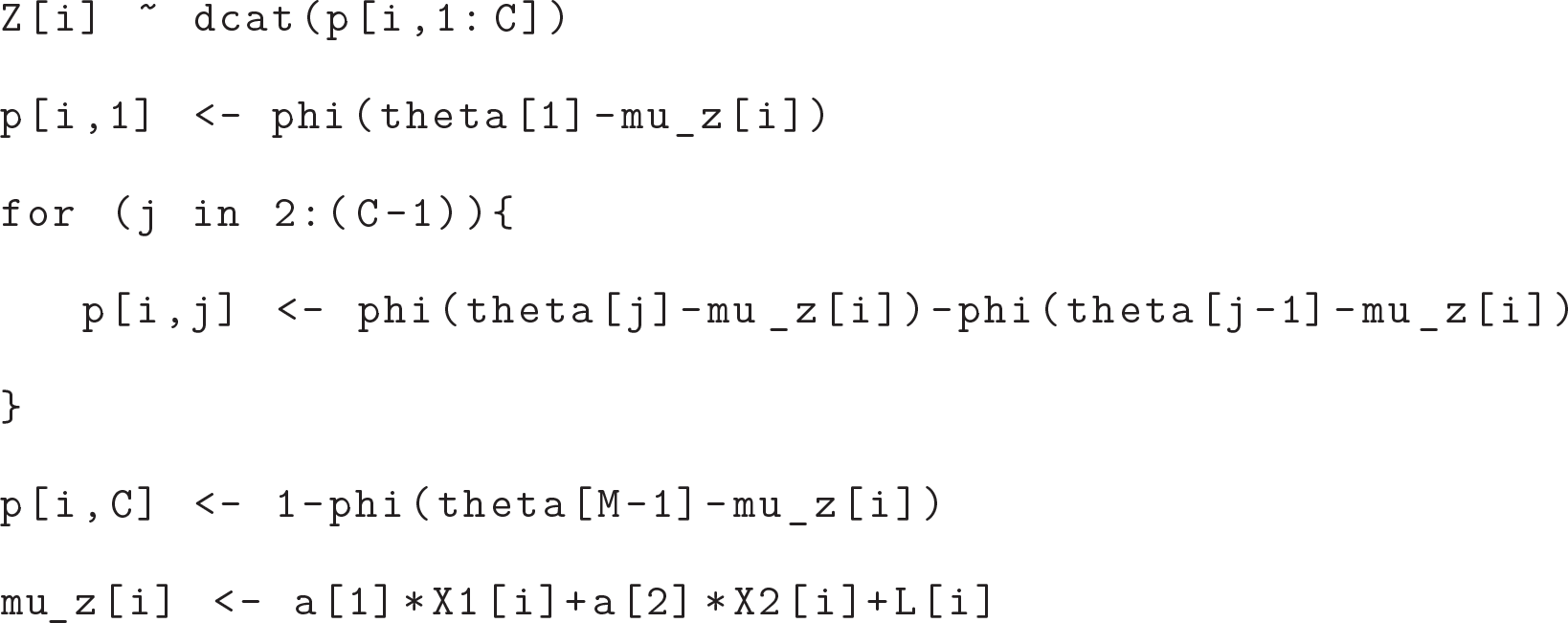
where dcat() is the categorical distribution and phi() is the Gaussian cumulative density function. Similarly,
For the latent variable L, we first assume underlying groups with corresponding probabilities for each component of L, so we have

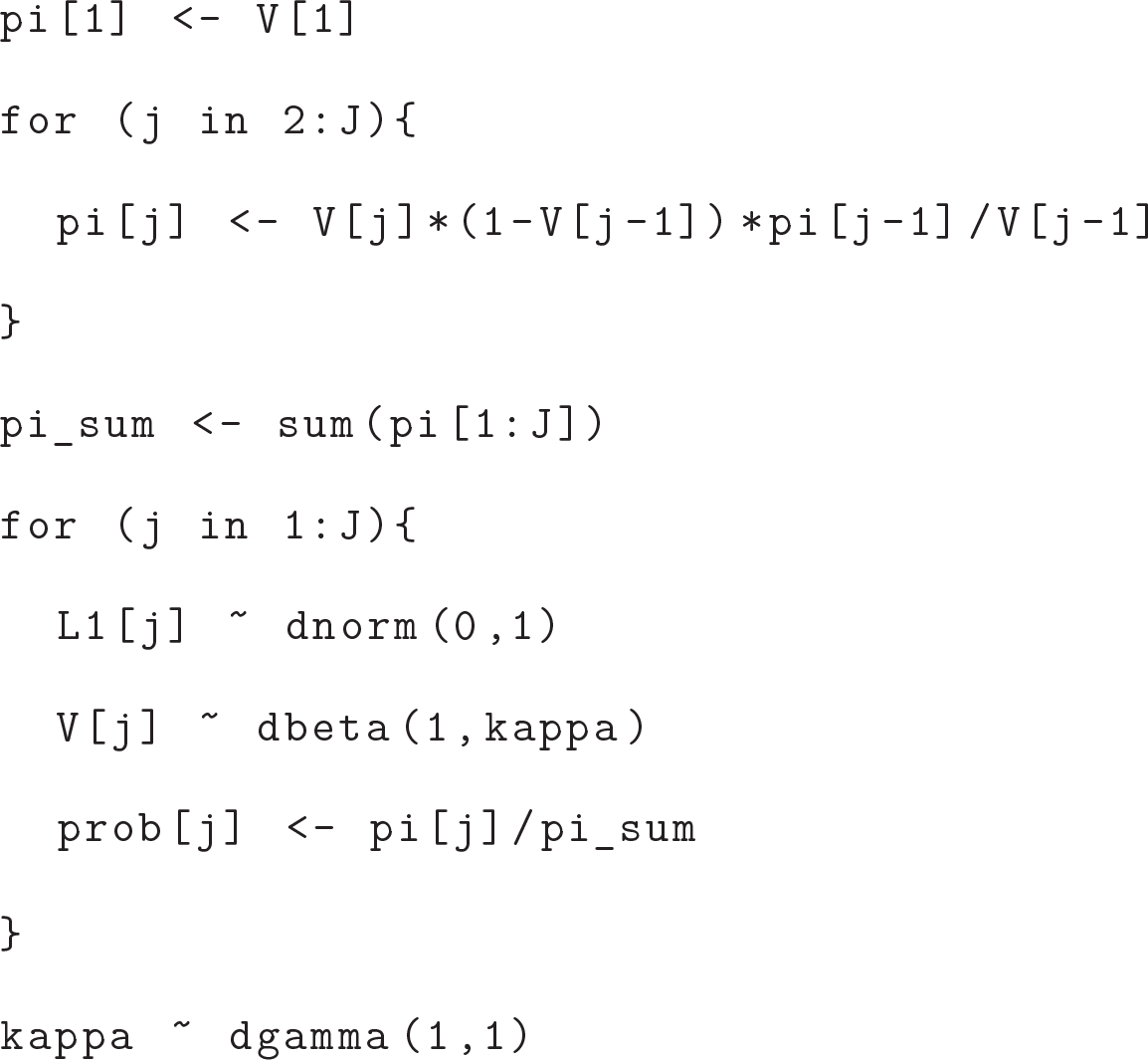
Aforesaid is the likelihoods in the for-loop. Outside the for-loop we should declare the priors for the unknown parameters. For the latent variable L, a finite-dimensional stick-breaking representation of the DP prior is assigned:
For priors of the thresholds of the ordinal response

Here, we should ensure that the thresholds are in an ascending order. However, nimble does not support the JAGS sort() syntax, so we have to write a nimble function to implement this. Fortunately, nimble provides ways to write self-defined functions just as in R by using a function nimbleFunction(). In addition, it can also call R functions with similar functionality using nimbleRcall(). Here we define a nimble function Rsort() by calling the R function sort() using nimbleRcall() as
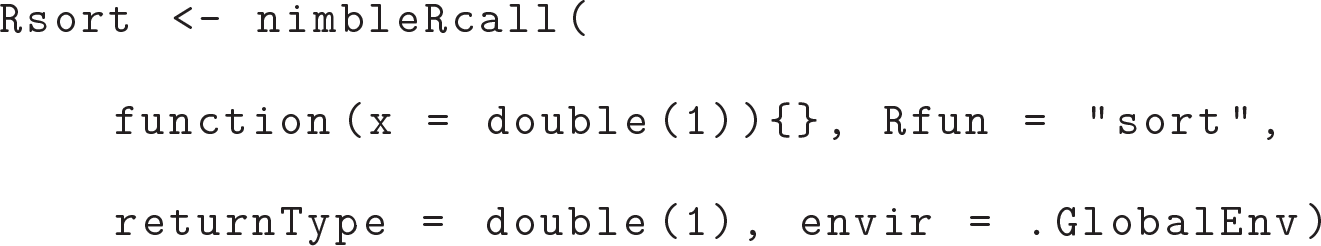
where ‘double(1)’ denotes the data type of the input and output. This self-defined function should be built before nimbleCode(). Finally the priors for
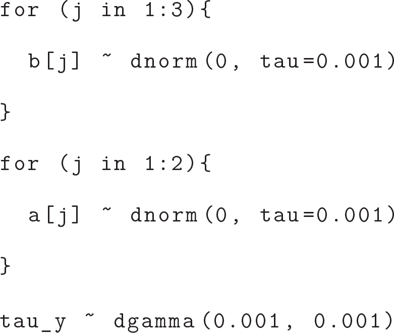
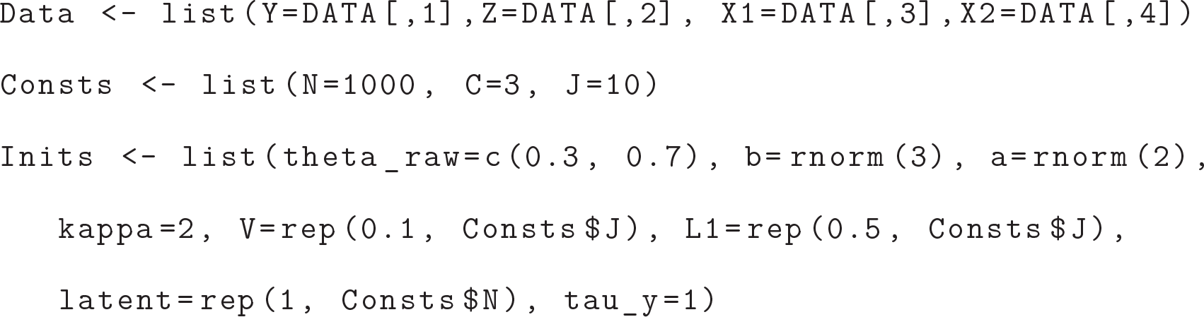
After defining the model code, we should define the constants, initial values and data list. Compared to WinBUGS and JAGS, data and initial values can be defined in the same way, while ‘constants’ is a new list that contains the values that would not change, including the variables that define for-loop indices. In our settings, the lists of data, constants and initial values are given as follows:
The second step is to build and compile the nimble model. The function nimbleModel() is used for the building the model and compileNimble() is used for compiling the model:

The function compileNimble() helps generating the C++ code, compiling that code and then loading it back into R, leading to faster computation. When running any nimble algorithms via C++, the model needs to be compiled before any compilation of algorithms, including MCMC algorithms.
Before we create the MCMC algorithms, we can see the default MCMC samplers that nimble assigned for the unknown parameters:

print=TRUE allows printing the MCMC samplers that nimble assigned for the parameters and thin=10 denotes the thinning interval. In our simulation study, the default samplers that nimble assigned for the precision parameter and the coefficient parameters of the continuous outcome
The next step is to create the MCMC algorithm by using the function buildMCMC(), and compile it again and then run it:
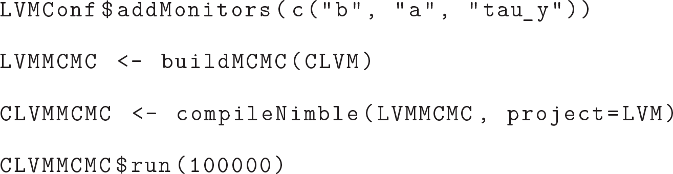
The function addMonitors() allows for declaring the parameters that we want to estimate and run() represents running the MCMC iterations. After that, we can obtain the MCMC samples, and then obtain the posterior estimates of the parameters.
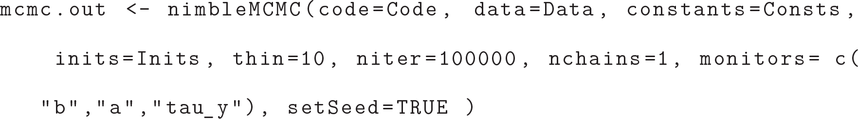
nimble also provides a one-line function of MCMC for the users to invoke the MCMC engine directly, which generally takes the code, data, constants and initial values as input, and provides a variety of options for executing and controlling multiple chains, iterations, thinning intervals, etc.
For the outputs, we can use another R package coda (Plummer et al., 2006) to summarize and generate plots just as in JAGS.
Application: Chinese General Society Survey 2013
In this section we applied our proposed model and method to analyse data from the Chinese General Society Survey (CGSS) 2013. CGSS, launched by the Department of Sociology of the Renmin University of China and the Survey Research Center of Hong Kong University of Science and Technology, is a survey project aimed at systematically monitoring the changing relationship between social structure and quality life in both urban and rural China. CGSS collects quantitative data about social structure, quality of life and the underlying linking mechanisms of these two aspects.
For this dataset, we considered two important variables, annual income (
In order to find out the factors that may have impacts on these two responses, we also considered the following explanatory variables: gender (
Summary of response and explanatory variables in CGSS 2013
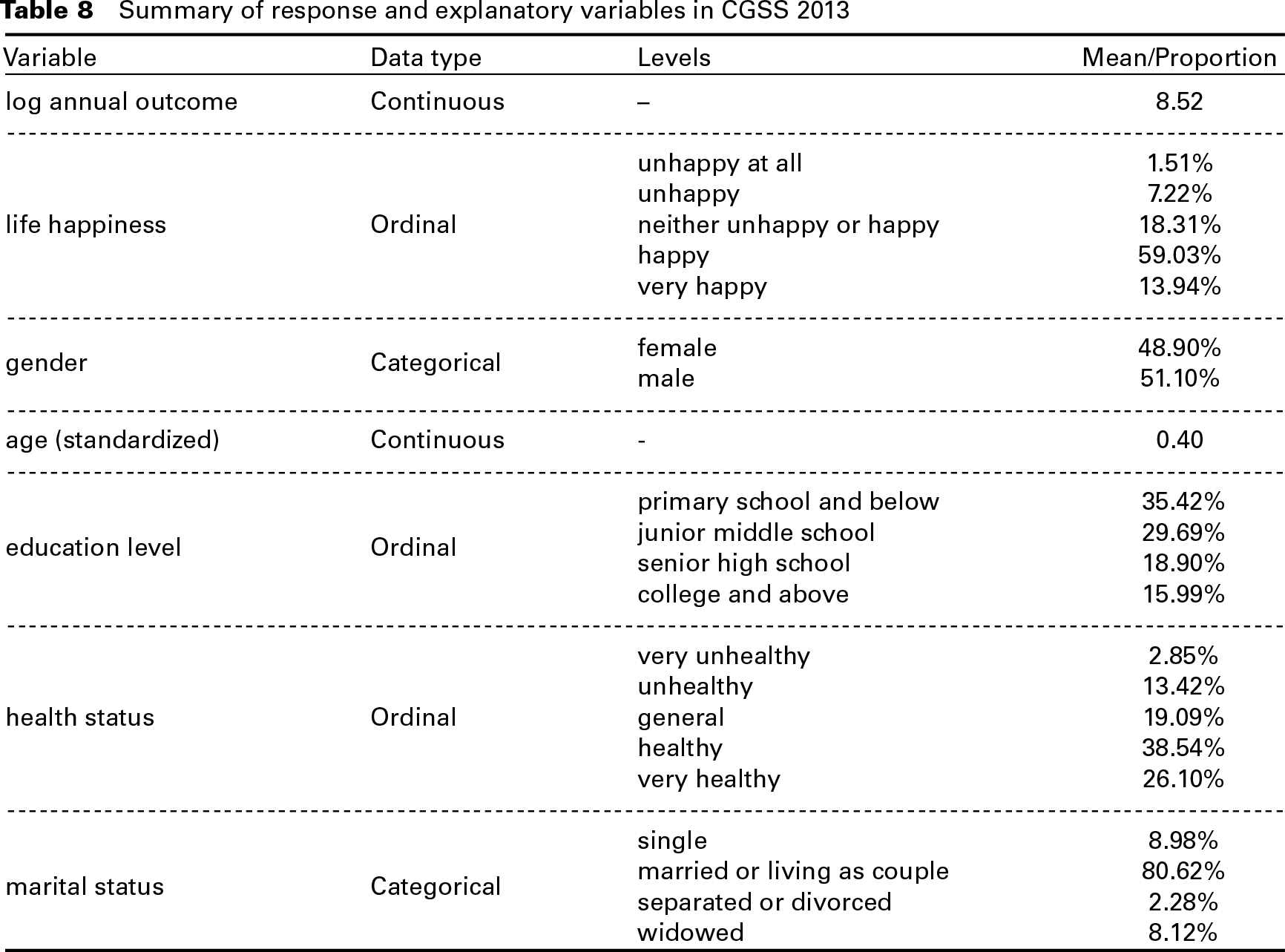
Summary of response and explanatory variables in CGSS 2013
Box plot of log annual income versus life happiness

The box plot of these two responses are shown in Figure 1. From Figure 1 we can observe that there is a tendency that with a higher level of life happiness, the annual income is higher. Therefore, we cannot assume these two variables are independent and analyse them separately. A joint analysis is more suitable for this circumstance. With the data described earlier, we set up the models for the mixed continuous and ordinal outcomes according to Section 2 as follows:
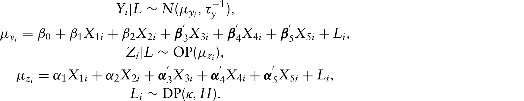
Since covariates education level (
For Bayesian implementation, priors on the unknown parameters are given as described in Section 3. R and nimble were used for programming, and a single Markov chain was used with the first 500 iterations being the burn-in phase and the remaining 5 000 samples used for posterior estimation. The thinning interval was set to be 10. Convergence was monitored by trace plots and ACF plots of the estimates.
We also assume different priors on L as M0–M4 in Section 4 and applied DIC and LPML for model selection. DIC and LPML values for these five models are shown in Table 9.
DIC and LPML values of the competing models for dataset CGSS 2013
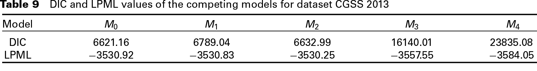
From the model comparison results, we can see that model M0 has the smallest DIC value, while LPML chooses model M2 as the best model. However, since there is a small difference between the LPML values of M0 and M2, the best model we choose for this dataset is M0. The Bayesian estimates of the parameters in model M0 are shown in Table 10. The traceplots and ACF plots of these parameters are given in the supplementary materials online.
Bayesian estimation of parameters in model M0
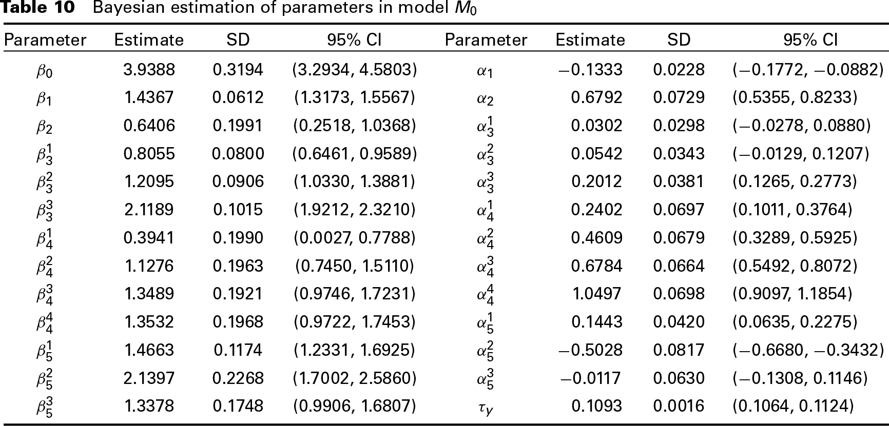
From Table 10, we can observe that at the 95% credible level, covariate gender has an impact on both the annual income and life happiness. Males tend to have higher annual income than females, but females have higher level of life happiness than males. Age has a positive impact on both annual income and life happiness, meaning that older people tend to have higher annual income and higher level of life happiness than younger persons. People with higher education level generally have higher annual income than people with lower education level. For life happiness, people who have been to college or above have significant improvement of life happiness than people of other education levels. People with a better health status tend to have higher income and higher level of life happiness. For different marital status, people who are single have a lower annual income than people of other marital status. The level of life happiness for people who are married or living as couples is the highest, and inversely, people who are seperated or divorced have the lowest level of life happiness.
In this article we focus on the use of DP as a prior for the latent variable in our joint model. However, the discreteness of DP makes the model not that appealing for all applications. When the unknown distribution is known to be continuous, the DP measures would be awkward for its discrete nature. For some hierarchical models, the DP prior may lead to inconsistent estimates if the true distribution is continuous (Rodriguez and Müller, 2013). In order to mitigate this limitation of DP, a convolution with a continuous kernel can be added to the discrete distribution, that is, assigning a DP mixtures of continuous distributions as a prior for the latent variable.
Suppose for the random samples of latent variables

where

where
The DP mixtures are countable mixtures with an infinite number of components and specific priors on the weights

which is equivalent to

The DP mixtures of normals prior allows a flexible continuous distribution for the latent variable. A normal distribution
In order to show the performance of DP mixtures prior, we also built the model using DP mixtures of normals prior with a logistic base function for the latent variable L to fit the simulated data in Simulation 1. Hyperpriors for
Simulation results of model M1* when L is actually bimodal

Simulation results of model M1* when L is actually bimodal
From Table 11, we can see that the bias and RMSE of the posterior estimates are relatively small and the CP values are all greater than 0.92, showing that the posterior estimates in model M1* are precise. By comparing the results of model M1 in Table 2, we can see that the bias of the estimates in model
In this tutorial article, a Bayesian semiparametric latent variable model with the latent variable following a DP prior is applied for joint modelling mixed continuous and ordinal outcome variables and the R package nimble is used for implementation. Through simulation study and an empirical analysis of data from CGSS 2013, it is indicated that the semiparametric LVM with DP prior and the model selection criteria perform well. Besides, an extension of DP prior to DP mixtures prior is introduced for greater flexibility.
There are several possible extensions that can be made to improve the current model. First, the current analysis is cross-sectional, so we can generalize the model to more complex data structures, including clustered data, longitudinal data, and other mixed types of outcomes. Second, the DP prior can be extended to DP mixtures prior introduced in Section 6, and it is also valuable to explore the performance of DP mixtures priors of different continuous distributions. Third, missing data are another important issue to be considered. Missing data are common in scientific research and simply ignoring or inappropriately handling these missing values would lead to biased estimates. With missing values, the analysis procedure will be more complicated, especially for non-ignorable missing values.
Supplementary Materials
Supplementary materials for this article, including the model code, the traceplots and ACF plots mentioned in Section 5, are available from
Declaration of conflicting interests
The authors declared no potential conflicts of interest with respect to the research, authorship and/or publication of this article.
Funding
This work was funded by Chinese National Program for Support of Top-notch Young Professionals (Grant number 2015338).