
Abstract
In this article, we analyse dependence structures among international trade flows of major conventional weapons from 1952 to 2016. We employ a Network Disturbance Model commonly used in inferential network analysis and spatial econometrics. The dependence structure is represented by pre-defined weight matrices that allow for correlating flows from the network of international arms exchange. Three dependence structures are proposed, representing sender-, receiver- and sender–receiver-related dependencies. The appropriateness of the presumed structures is comparatively assessed using the Akaike Information Criterion (AIC). It turns out that the dependence structure among the arms trade flows is complex and can be represented best by a specification that relates each arms trade flow to all exports and imports of the sending and the receiving state. Controlling for exogenous variables, we find that the trade volume increases with the GDP of the sending and the receiving state while the impact of geographical distance, regime dissimilarity and formal alliance membership is rather small.
Introduction
In this article, we investigate international trade flows of Major Conventional Weapons (MCW) using data provided by the Stockholm International Peace Research Institute (SIPRI). MCW include armoured vehicles, aircraft, naval vessels etc., and SIPRI has compiled all international arms transfers from 1950 to 2016 in a comprehensive database. It includes the sending and the receiving country as well as the volume of the trades in a certain year. The volume is measured as so-called TIV, i.e. trend-indicator value(s), and represents the military value and the production costs of the transferred products. The data can be regarded as a year-wise sequence of weighted networks where the countries are the nodes and the arms trade flows among them are the valued edges.
Several scholars have started to investigate arms trade using a network framework, but the available studies were restricted to binary relations, that is, trade or no trade, see for example Akerman and Seim (2014), Kinne (2016), Lebacher et al. (2018) and Thurner et al. (2018). The workhorse in inferential binary network analysis is the Exponential Random Graph Model (ERGM), as introduced by Holland and Leinhardt (1981) (see also Frank and Strauss, 1986; Kolaczyk, 2009; Lusher et al., 2012). Recent proposals for modelling valued networks within the ERGM class have been provided by Krivitsky (2012), or by Desmarais and Cranmer (2012) having proposed the Generalized Exponential Random Graph Model (GERGM). The first model is actually designed for count data while the GERGM approach allows for continuous edge weights. Both approaches are not suitable for modelling arms trade data because the TIVs are continuous and heavily zero-inflated (i.e., TIV
The analysis of the binary event of an arms transfer is important since trading of arms implies governmental agreement and therefore indicates direct and indirect trust relations (see, e.g., Jackson, 2010), regardless of the amount of trading. In this article, however, we focus on the amount of trading. This objective raises the question of how to handle the high share of structural zeros (approximately 98%) because this poses substantial problems in conventional edge-based network models. Following models for insurance claims, where the amount of the claim is modelled conditional that there is a claim (Frees and Valdez, 2008), we opt for excluding the decision to trade arms and to focus only on the amount of trading, given that there is trading (i.e., TIV
The article is organized as follows. In Section 2, we give a short description of the data, while in Section 3, we explain the shortfalls of recently proposed models for valued networks in view of our dataset. In Section 4, we introduce our model and propose different specifications and explanations for possible dependence structures. In Section 5, we present the results of our analysis. Section 6 concludes the article. Data,
Data description
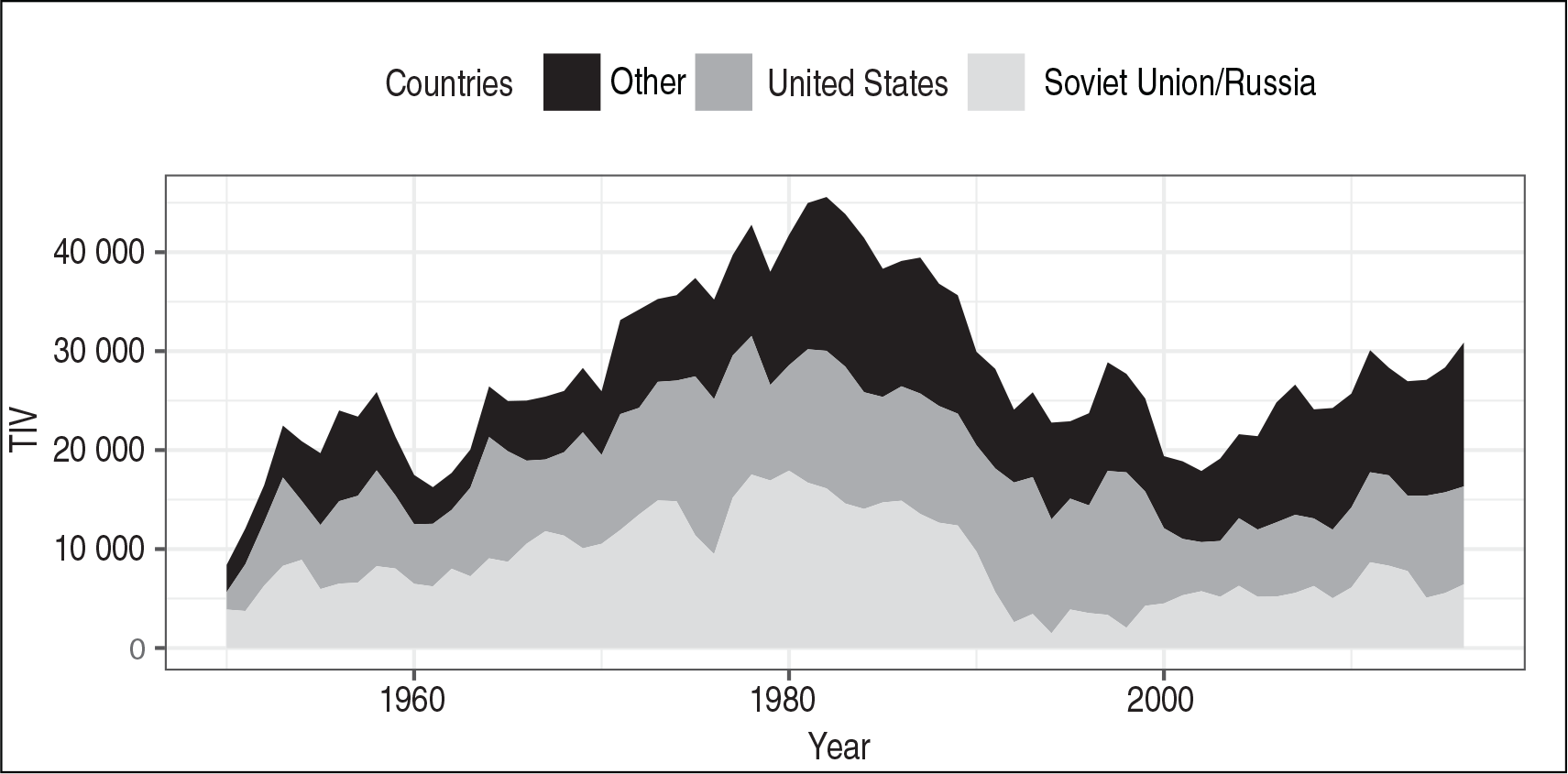
Development of the exported TIV for 1950–2016 for the United States, Soviet Union/Russia and all other countries
Development of the exported TIV for 1950–2016 for the United States, Soviet Union/Russia and all other countries
The Stockholm International Peace Research Institute (SIPRI) is a unique data source for the international transfers of major conventional weapons. It covers more than 200 countries from 1950 to 2016, and includes the types and TIV volumes of MCW that are traded. Table 2 in the Appendix gives an overview of weapon systems included. The advantage of the TIV measure is consistency over time and comparability of different arms systems. (For a detailed description of the data and methodology, see SIPRI (2017b) or Holtom et al. (2012). The database can be accessed online at SIPRI (2017a))
Log-log plot of aggregated TIV export versus outdegree (left) and aggregated TIV import versus indegree (right). The solid line in the middle represents the mean of exports or imports for a given in- or outdegree. Lower and upper bounds indicate minimum and maximum values
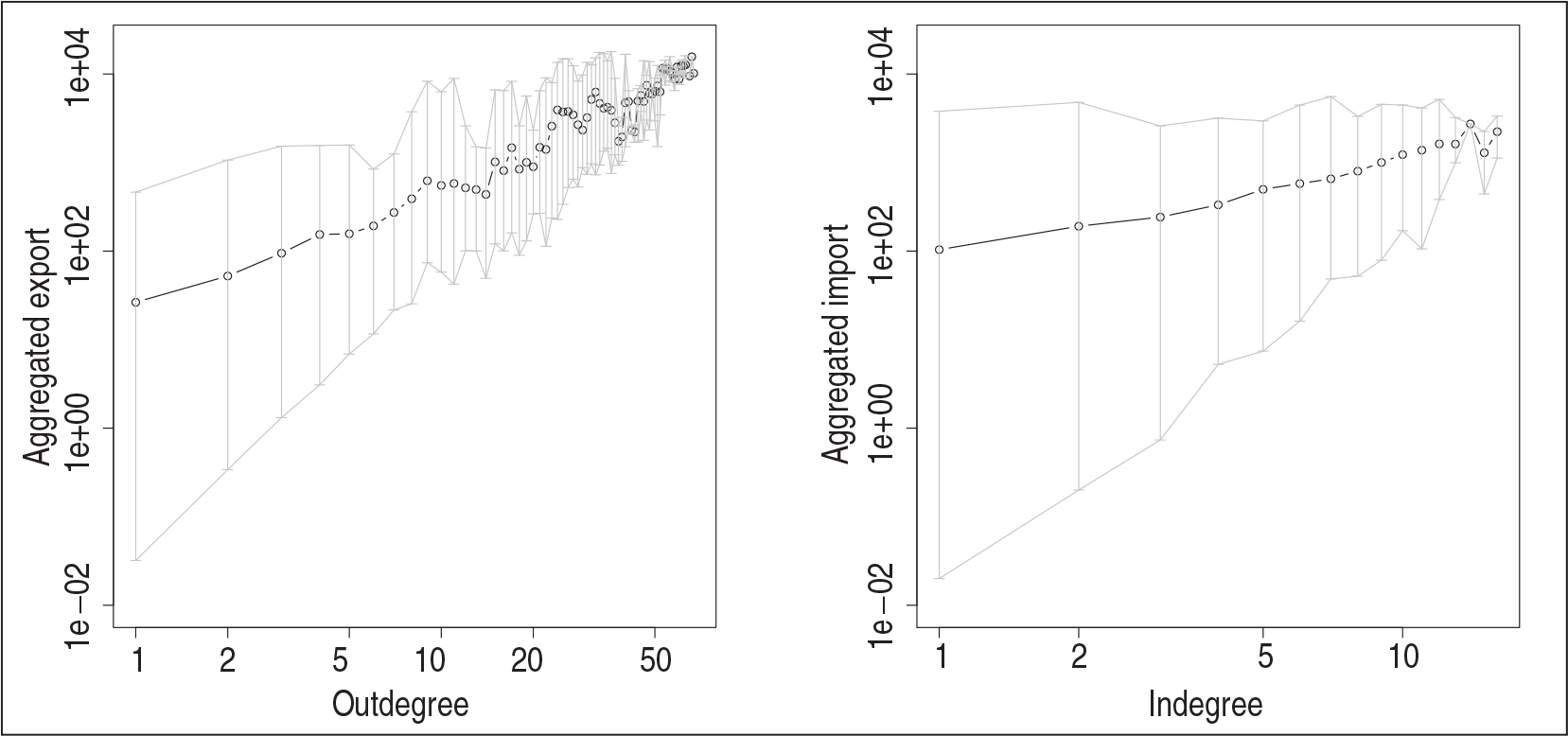
In Figure 1, the evolution of the aggregated TIV is shown. The contribution of the two most important exporters, namely the United States and the Soviet Union (Russia since 1992), is separately coloured. Figure 2 relates the outdegree (i.e., number of out ward directed binary relations) and indegree (i.e., number of inward directed binary relations) in a log-log plot to the aggregated export and import volumes, respectively. In terms of the slope and range (i.e. the distance between der lowest and the highest value), it can be seen that the connection between aggregated export volume and the outdegree is somewhat stronger than the relationship between import volume and indegree. Nevertheless, both volumes increase on average in the respective degree.
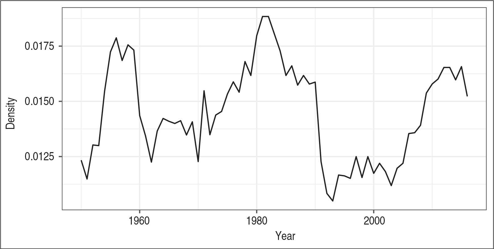
The modelling approach of Krivitsky (2012) allows for count data and is therefore not directly suitable for arms trade data since the TIV are continuous. The GERGM (Desmarais and Cranmer, 2012), however, is applicable to networks with continuous edge weights but suffers from two major restrictions when being applied to our dataset. The estimation, even for networks of moderate size, can be computationally very demanding, or even proved to be infeasible as also noted, for example, by Simpson et al. (2013), Ward et al. (2013), Simpson and Laurienti (2015) and Boivin and D'Elia (2017). In our application, we have 65 yearly networks with up to 160 nodes in the most recent periods, rendering estimation impossible in an acceptable amount of time. But even if we were able to handle the numerical problems, an unsurmountable obstacle constitutes the extreme number of zero-valued trades that arises if we create a weighted adjacency matrix and code all non-existing transfers as zero. Figure 3 shows the density of the networks for the whole observational period. Even in the years with the highest density, we have roughly 98% zeros in the data, excluding the possibility to use a GERGM. As indicated also in Schoeneman et al. (2017), the GERGM model cannot handle zero-inflated data.
Network density (share of realized trade relations as compared to all possible trade relations) from 1950 to 2016
Network density (share of realized trade relations as compared to all possible trade relations) from 1950 to 2016
An alternative approach for valued networks are latent space models (see, e.g., Hoff et al., 2002; Handcock et al., 2007). This model class assumes that the endogenous network dependencies can be accounted for by representations of the nodes in a latent space. Obviously, the approach is tempting because it allows for an interpretation as in generalized linear models conditional on the latent space. In addition, latent space models were already applied in trade research (see Ward and Hoff, 2007; Ward et al., 2013; Berlusconi et al., 2017). The approach comes, however, with some disadvantages. First, the zero-inflation problem poses again a major obstacle. We applied the routines in the
Provided we focus exclusively on observed trade, we can apply models from the family of spatial econometric models in order to detect related transfers. Here, two canonical models can be distinguished, the spatial autoregressive (SAR) model and the spatial error model (SEM). The main difference between the SAR model and the SEM is related to the assumptions on how the network structure influences the outcome. In the SEM, we have the same interpretation of the coefficients as in the linear model, whereas in the SAR model, changes in the covariates affect all related transfers (LeSage and Pace, 2009; Kauermann et al., 2012). This implies, for example, that if the logarithmic GDP of the sender has a positive coefficient, and two transfers
Definitions and basic formulation
In
As a tool to analyse the dependence structure among

The information given in the neighbourhood can be summarized in a
Regression model
Arms trade flows are non-negative, leading us to consider a multiplicative model of the form
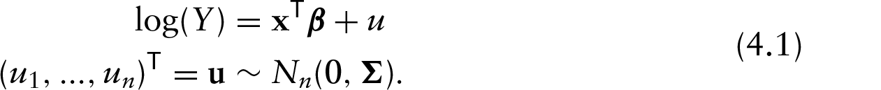
Here,

where

This implies the covariance matrix
We describe now the central modelling task, i.e. the appropriate specification of matrix
Directed valued network of arms trade in 1952. Edges (nodes) are scaled proportional to the logarithmic exports (logarithmic aggregated exports) measured in TIV
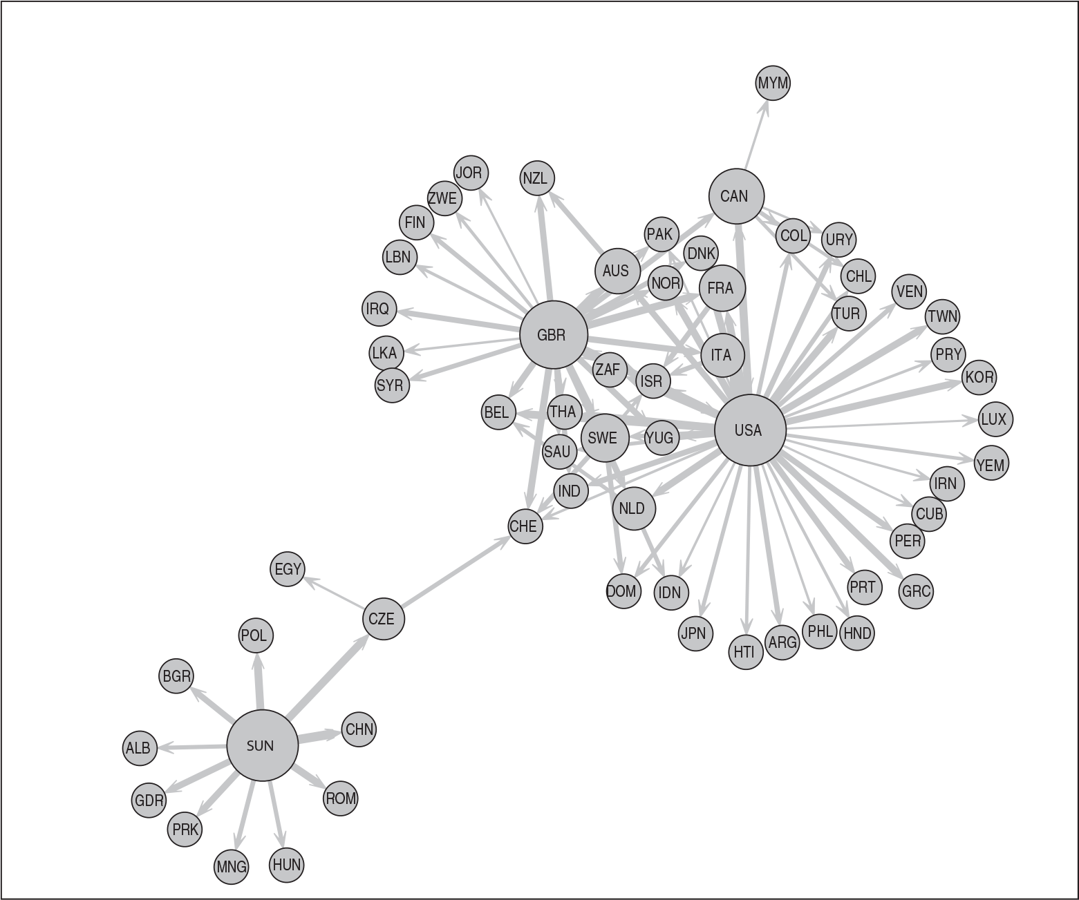
Directed valued network of arms trade in 1952. Edges (nodes) are scaled proportional to the logarithmic exports (logarithmic aggregated exports) measured in TIV
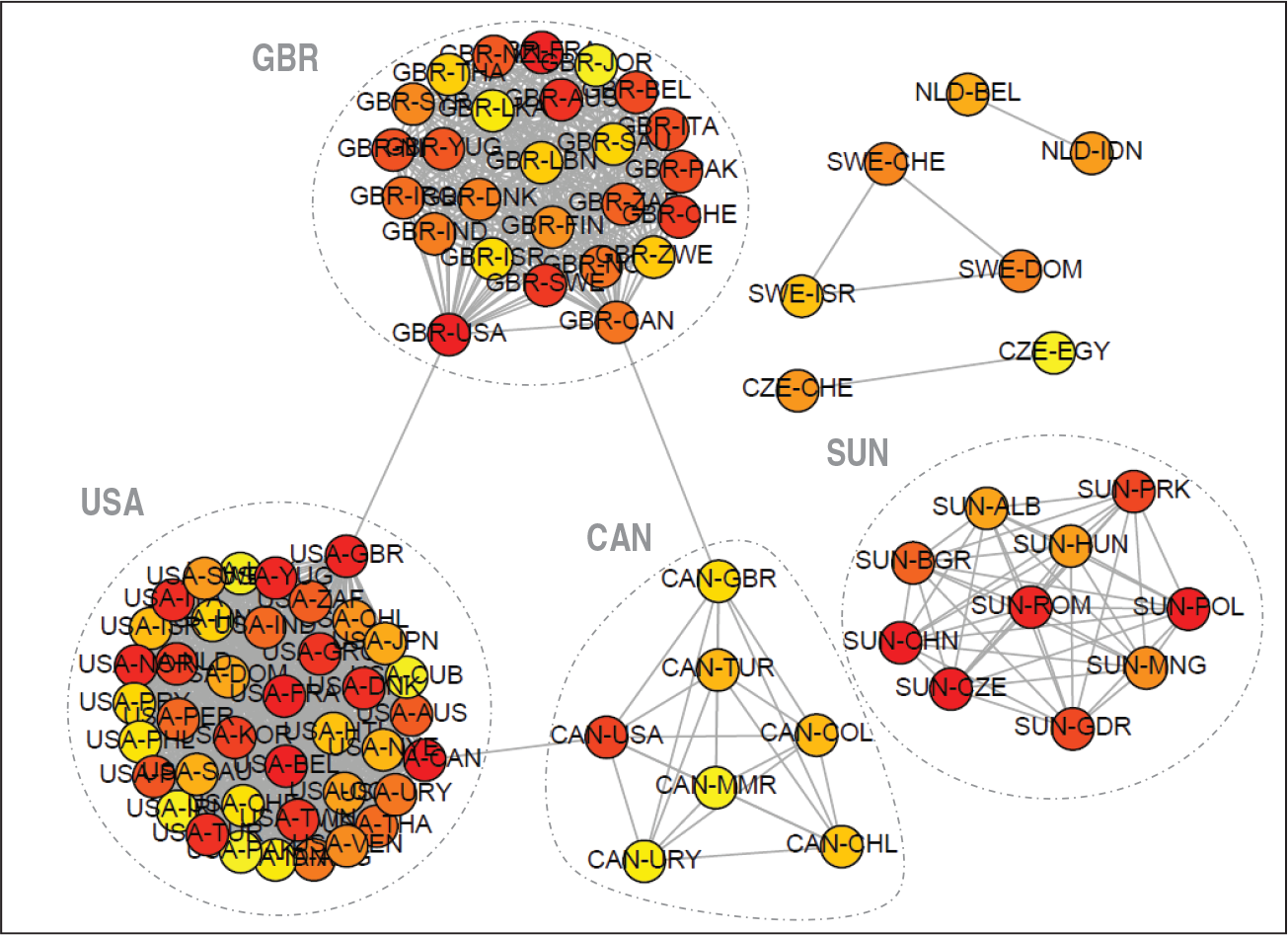
Armstradecorrelation
The first dependence structure relates an arms trade flow from country

The corresponding graph representation for the year 1952 is shown in Figure 5. The trade flows are grouped within clusters that are related to specific exporting countries, most notably they consist of the trade clusters of the big exporters: United States (USA), United Kingdom (GBR), Canada (CAN) and the Soviet Union (SUN). Through the dependence on reciprocal flows, the clusters are connected among each other if there is between-cluster trade. This explains the connection between the cluster of the United States (USA), Great Britain (GBR) and Canada (CAN). The trade activity of the Soviet Union (SUN), however, is disconnected.
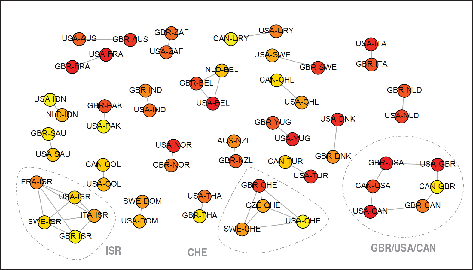
Armstradecorrelation
The aforementioned concept can be amended such that the armstradecorrelation of an arms trade is related to the trades of the importing country and not to those of the exporting one. This would imply the hypothesis that there exist countries that are strong importers and countries that import small volumes. Additionally, we take into account reciprocity with the same arguments as above. This means

and entails that the arms trade amount from
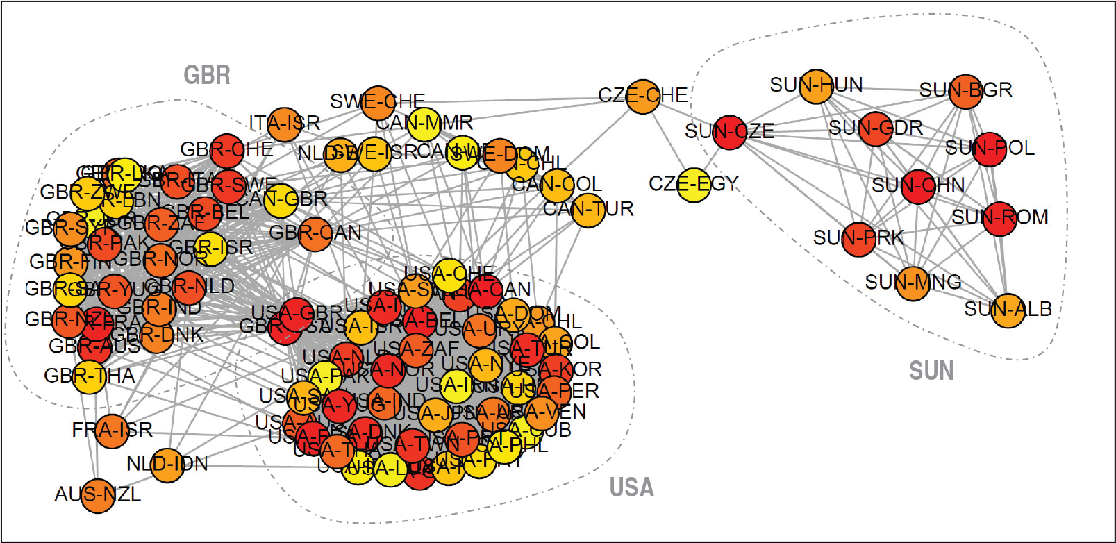
Armstradecorrelation
The structures of the previous tradecorrelations can be combined by the inclusion of the whole trade activity of

In this case, an arms trade from country
We control for the influence of economic and political quantities and of geographical distance by including additional covariates in model (4.1). Since there is an average time lag of roughly two years between ordering and delivering of weapons and some covariates are only available from 1950 onwards, the first network under study is the one of 1952, and covariates are lagged by two years.
Economic variables: The standard measure for economic size is the gross domestic product (GDP). We consider this as a measure of market size and include it in logarithmic form for the sender as well as the receiver. Real GDP is measured in thousands of USD. Data until 2010 are taken from Gleditsch (2013a). Data for later years are drawn from the World Bank real GDP dataset (see The World Bank, 2017).
Distance: Gleditsch (2013b) provides data on the distances between capital cities measured in kilometres. We include this measure for the physical distance between countries
Political variables: We use a dummy variable being one if the countries
This choice of covariates is in line with recent empirical (Akerman and Seim, 2014; Martinez-Zarzoso and Johannsen, 2017; Bove et al., 2018; Thurner et al., 2018) and theoretical (Garcia-Alonso and Levine, 2007) arms trade research. It builds on a modelling approach similar to the gravity equation, a very common parsimonious structure for the analysis of international trade flows (Disdier and Head, 2008; Ward et al., 2013; Head and Mayer, 2014; Egger and Staub, 2016).
Results
Model selection
Our ultimate goal is to select a suitable dependence model from Section 4.3 As recommended by Leenders (2002) for this model class with several candidate weight matrices, we compare the proposed models using the Akaike Information Criterion (AIC) (see, e.g., Claeskens and Hjort, 2008). A simulation study in Section 5.4 shows that this is a valid strategy for identifying dependence structures.
For comparison, we also include a simple linear model with unstructured error term (OLS,
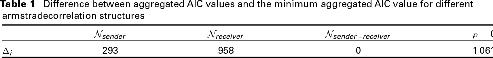
Difference between aggregated AIC values and the minimum aggregated AIC value for different armstradecorrelation structures
Difference between aggregated AIC values and the minimum aggregated AIC value for different armstradecorrelation structures
We see that the specification where ρ is restricted to zero (OLS) is among those models that have a very low probability of being the best one. Only in the years 1990–2000, the probability for this model rises substantially as a consequence of the collapse of the Eastern Bloc. This mirrors the fact that this major event broke up long established network structures. Overall, the low probability for the restricted model provides evidence for our initial hypothesis that the trade flows are indeed correlated. For the armstradecorrelation structure that is related to the receiver (
Annual Akaike weights for different specifications (raw values in grey, smoothed in black)
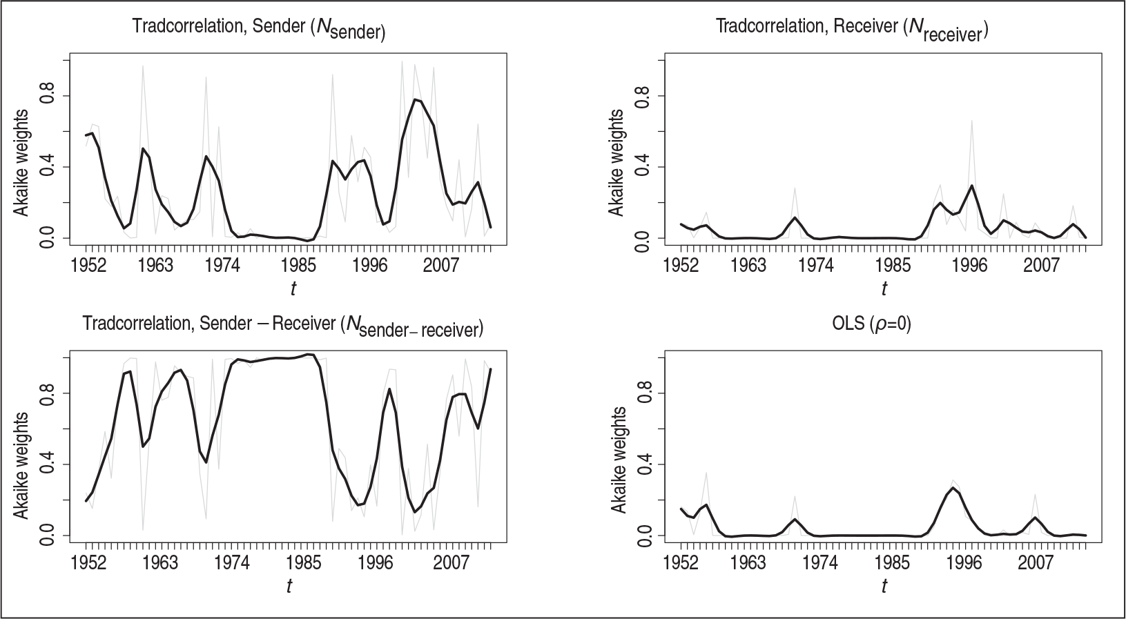
The two specifications that compete to be the best representation of dependencies are tradecorrelations
We take this as a clear evidence that the exchange of international arms leads to a rather complex dependence structure. This corroborates existing binary network analyses (see Thurner et al., 2018) and shows that, the assumption of independent observations, given the covariates, is a strong simplification of the real process. Based on these promising results, we continue to analyse the model with armstradecorrelation structure
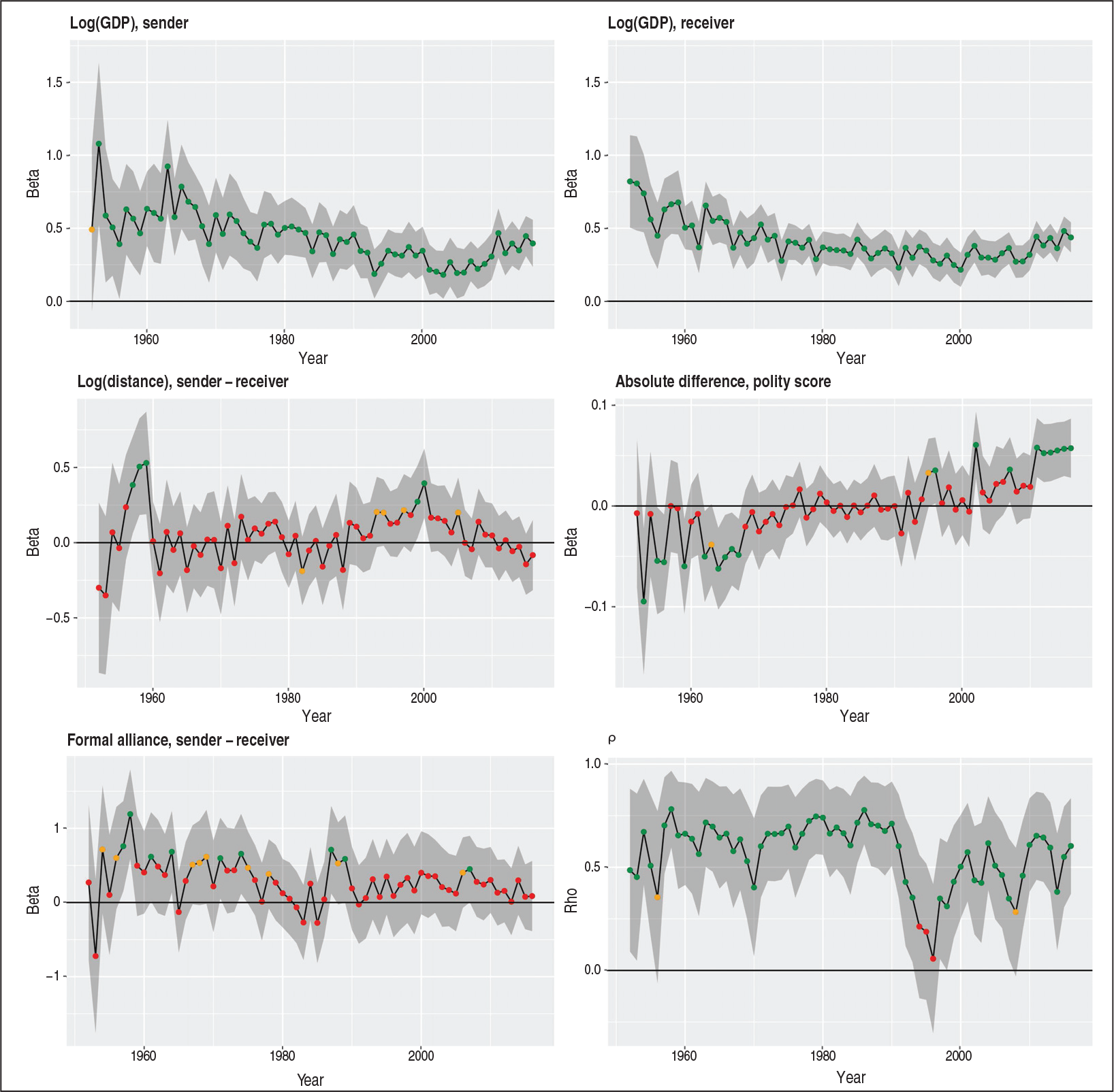
Economic variables: The coefficient on the logarithmic GDP of the sender is, with the exception of the year 1952, consistently positive and significant, showing a slight tendency to decrease with time. This can be seen from Figure 9, left panel, top plot and reflects the fact that countries with greater economic size have a higher tendency of possessing a highly developed arms industry and are able to produce and export expensive military equipment. When it comes to the GDP of the receiver (right panel, top plot), we also see a slight downward trend of the coefficients. As a rule, the coefficient is always positive and significant and comparable in size to the GDP of the exporter, that is, the economic size of the importer is also an important determinant of its import volume.
Distance: In the left panel at the middle plot of Figure 9, it can be seen that the coefficient related to the distance is mostly insignificant and even positive when significant.
Political variables: Before 1990, having an alliance (left panel, bottom plot) in tendency increased the amount of arms trading, but at least since 1990, this effect is almost zero. The coefficient on the absolute differences of the polity score (right panel, middle plot) shows a time-related trend. In the beginning (1953–1973), the coefficient is rather less than zero, giving the intuitive result that differences in political regimes reduce the amount of arms traded. From 1976 to 1991, the coefficient can be regarded as zero, which mirrors the fact that at the height of the Cold War, the belonging to a political bloc was more important than distances in the polity scores. After the end of the Soviet Union, the coefficient remains close to zero until 2011 where the coefficients become significantly positive for six consecutive years, providing the surprising result that differences in the polity score do not lead to a reduction of the traded amount of arms contrary to recent results of a study on the binary decision to trade (see Thurner et al., 2018).
Armstradecorrelation: The bottom right panel of Figure 9 shows the trade correlation coefficient using the structure
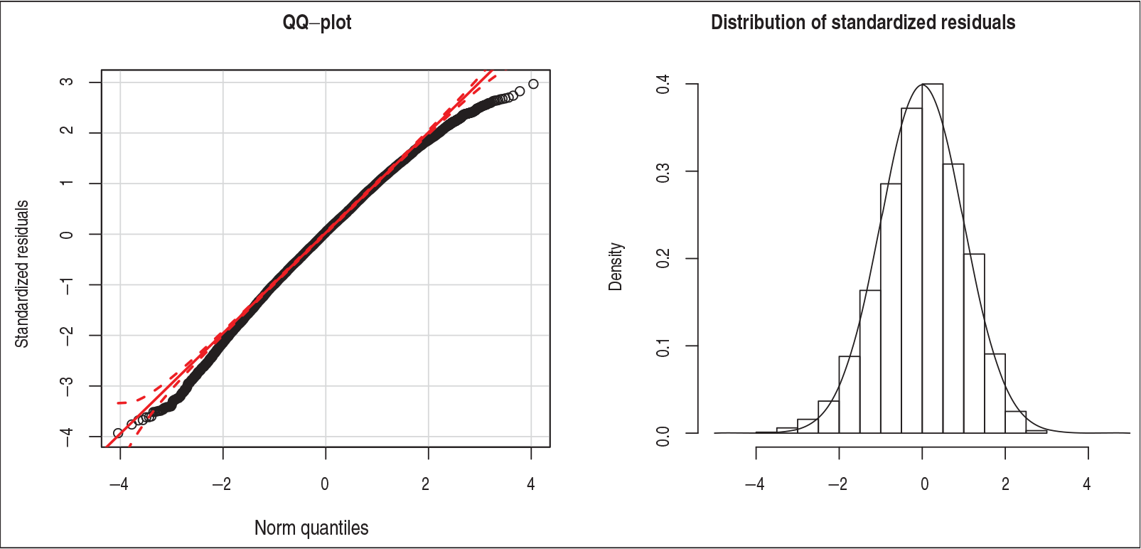
QQ-plot (left) and histogram (right) of standardized residuals
QQ-plot (left) and histogram (right) of standardized residuals
We give a graphical summary in Figure 10 for the pooled unstructured estimated residuals
Kernel density estimates of the armstradecorrelation residuals for selected countries in the time periods 1952–1991 (left) and 1992–2016 (right)
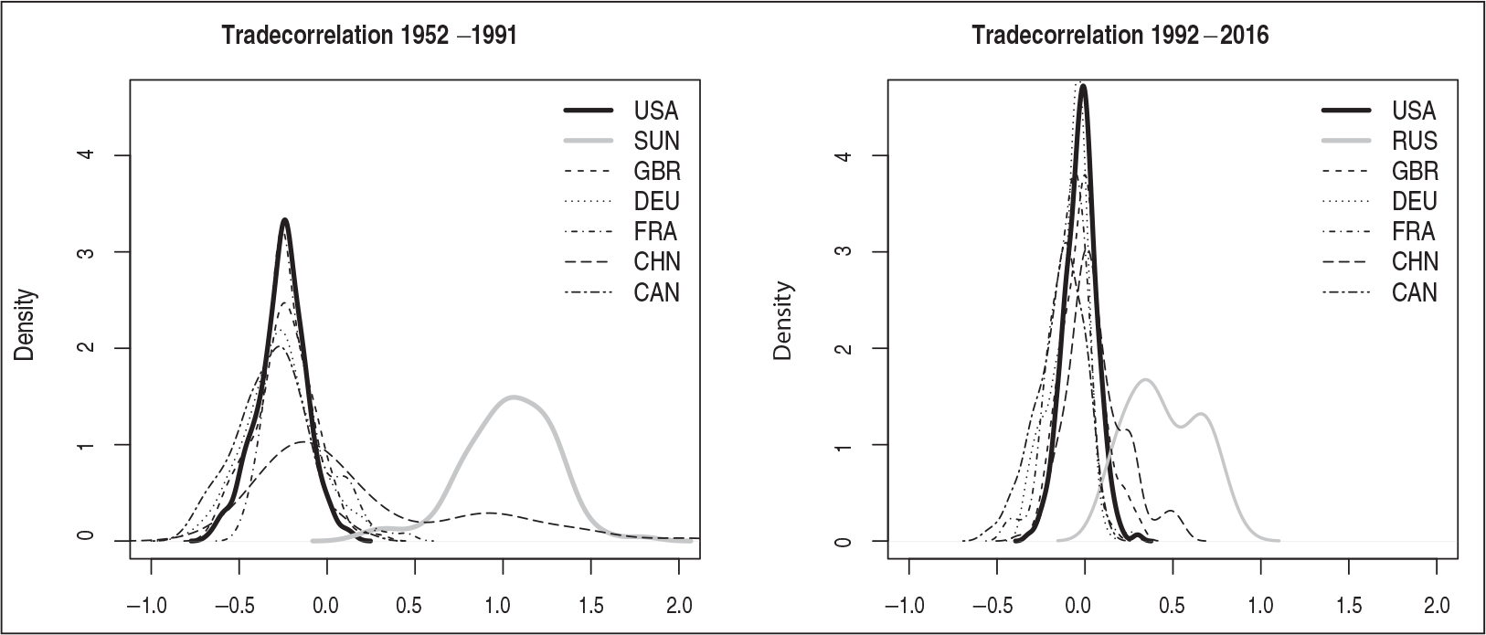
As shown in the previous section, the coefficient on the armstradecorrelation structure
In the following simulation study, we show that our model selection approach is suitable for the identification of appropriate dependence structures.
We take the binary arms trade networks from 1952 to 2016 as given and specify four different data generating processes (DGPs) for the arms trading amount in order to make the simulation study as comparable to the real analysis as possible. The DGPs are as follows:

where the covariates
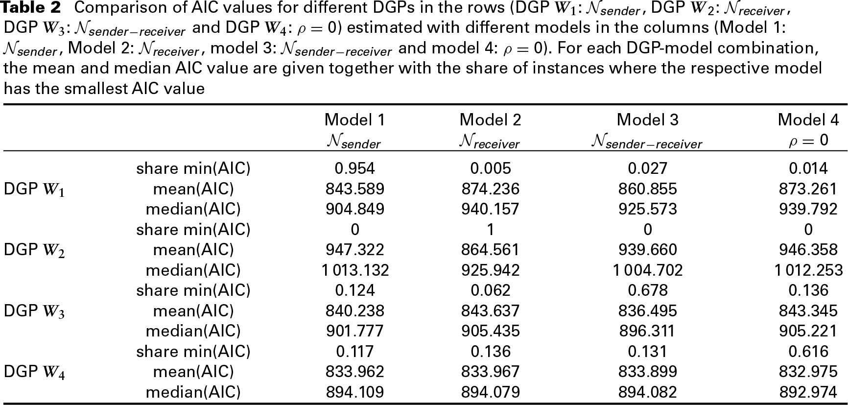
Comparison of AIC values for different DGPs in the rows (DGP W1: Nsender, DGP W2: Nreceiver, DGP W3: Nsender−receiver and DGP W4: ρ = 0) estimated with different models in the columns (Model 1: Nsender , Model 2: Nreceiver , model 3: Nsender−receiver and model 4: ρ = 0). For each DGP-model combination, the mean and median AIC value are given together with the share of instances where the respective model has the smallest AIC value
Comparison of AIC values for different DGPs in the rows (DGP W1: Nsender, DGP W2: Nreceiver, DGP W3: Nsender−receiver and DGP W4: ρ = 0) estimated with different models in the columns (Model 1: Nsender , Model 2: Nreceiver , model 3: Nsender−receiver and model 4: ρ = 0). For each DGP-model combination, the mean and median AIC value are given together with the share of instances where the respective model has the smallest AIC value
In a first step, we simulate all four DGPs 100 times for each of the 65 real binary networks. This provides us
In this article, we analysed the volume of international arms trade flows by employing a Network Disturbance Model. Three different dependence structures are proposed, and the best one is selected based on the minimization of the AIC. Using this approach, we find that a specification that relates the error term of an arms trade flow to the whole trade activity of the sending and receiving state performs well in most years. This indicates that the network of international arms trade exhibits a very complex dependence structure among the arms trade flows. The analysis of the armstradecorrelation coefficient shows that the correlation pattern among the flows is rather stable and breaks only for the transition period after the end of the Cold War. The development of the coefficients of the covariates discloses how the influence of economic and political factors has changed with time.
From a political economy perspective, the evolution of the coefficients on the covariates corroborates earlier results with respect to GDP. It does, however, yield surprising results on the distance measure and on political variables. Whereas the low influence of geographic distance confirms recent results from the analysis of the binary arms trade network (see Thurner et al., 2018), the low impact of regime dissimilarity (absolute difference of polity scores) and formal alliance membership stands in contrast to the effects on the formation of binary network ties and provides the new insight that regime dissimilarity and joint alliance membership are seemingly more important for the tie formation than for the volume of arms transfer given they trade.
Acknowledgements
We would like to thank SIPRI, and especially Siemon Wezeman for providing data and detailed information on the underlying data collection approach. This article has profited from the COST Action CA15109 European Cooperation for Statistics of Network Data Science (COSTNET), supported by COST (European Cooperation in Science and Technology). We thank two anonymous reviewers for their careful reading and useful suggestions.
Declaration of conflicting interests
The authors declared no potential conflicts of interest with respect to the research, authorship and/or publication of this article.
Funding
The authors acknowledge the financial support by the German Research Foundation (DFG) under grants TH 697/9-1 and KA 1188/10-1 ‘International Arms Trade: A Network Approach’.
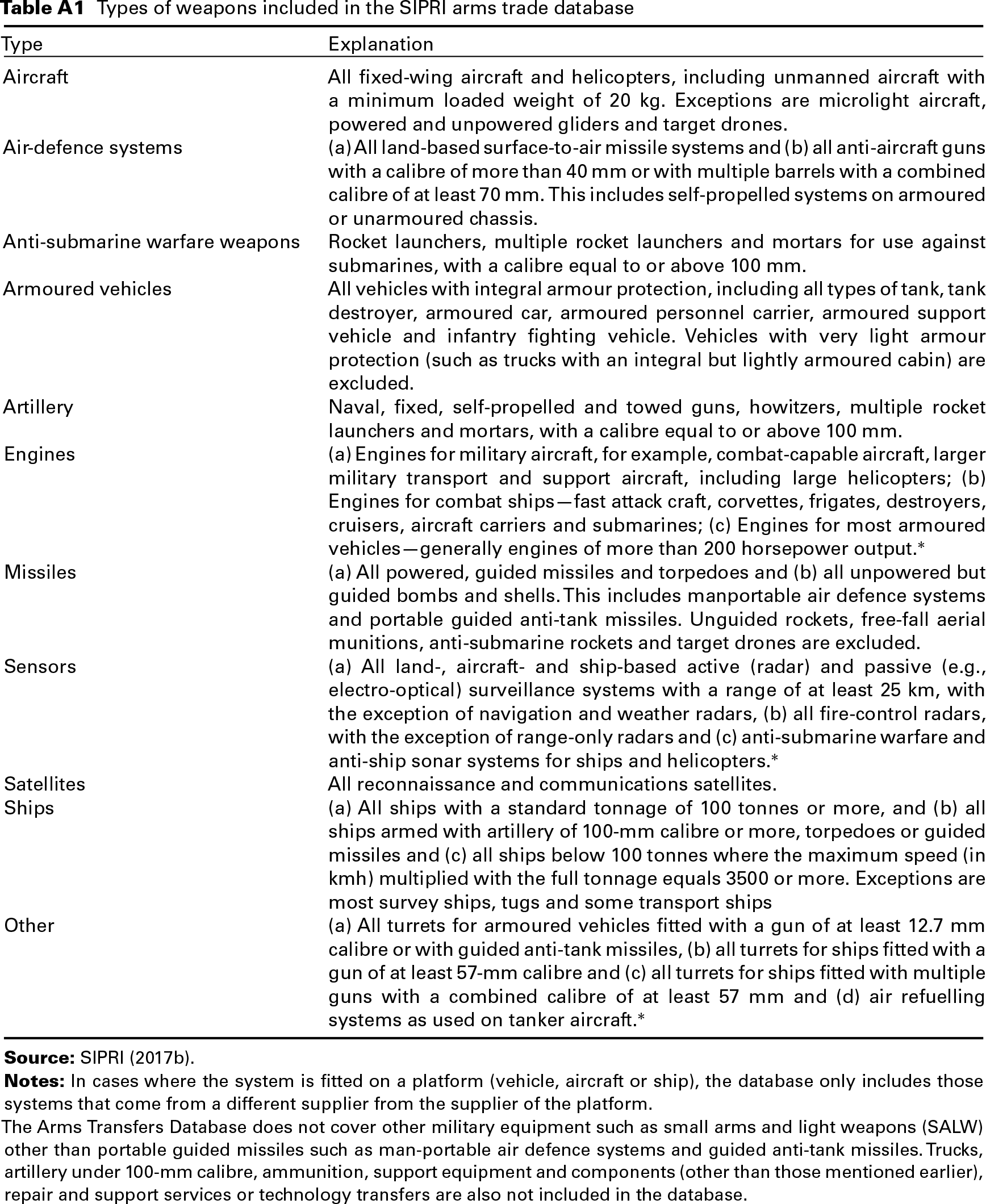
Types of weapons included in the SIPRI arms trade database
Types of weapons included in the SIPRI arms trade database
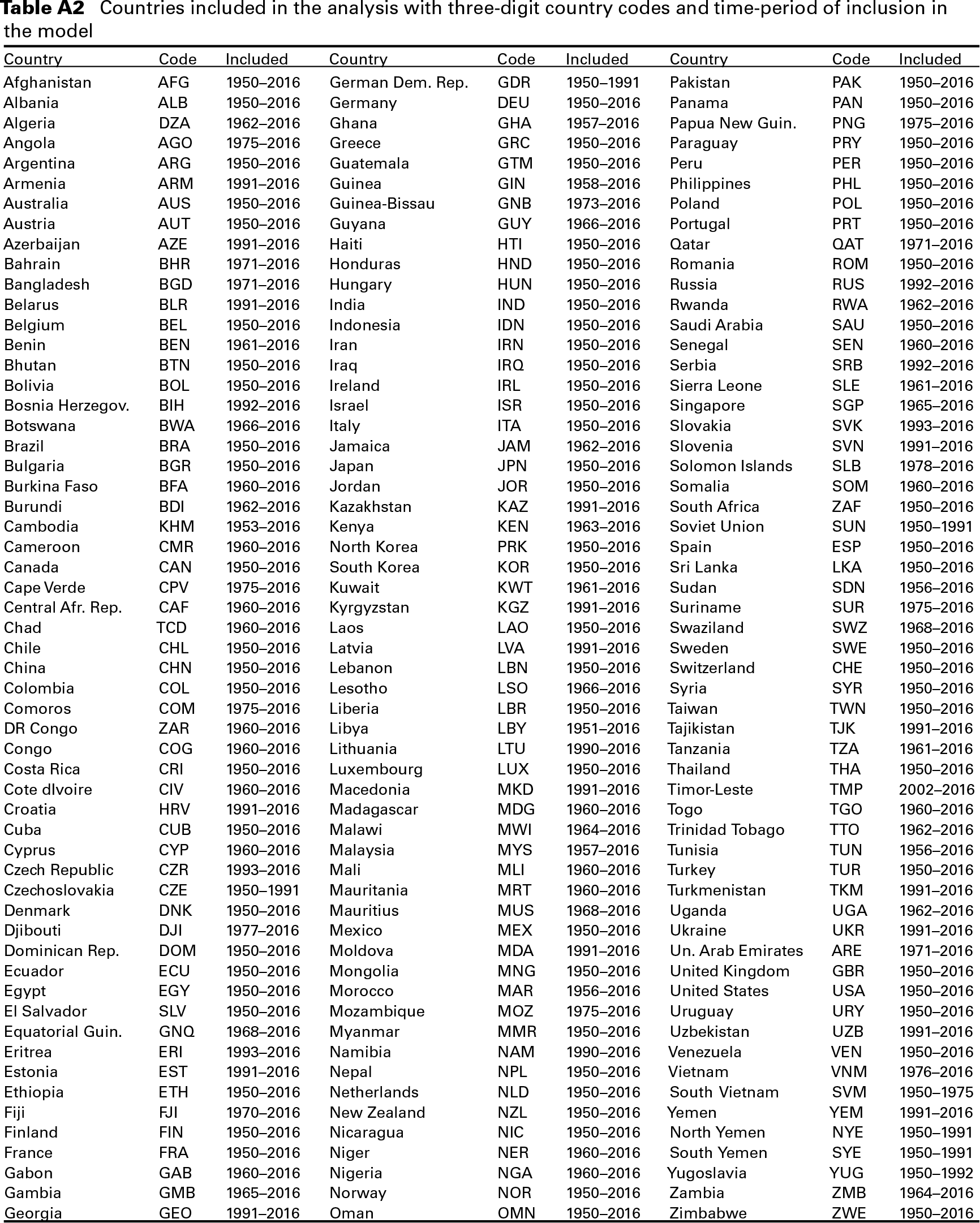
Countries included in the analysis with three-digit country codes and time-period of inclusion in the model
Appendix
Table 2 gives the categories of arms that are included in the analysis. All types with explanations are taken from SIPRI (2017b). The 171 countries that are included in our analysis can be found in Table 3, together with the three-digit country codes that are used to abbreviate countries in the article. In addition, the time periods, for which we coded the countries as existent are included. Note that the SIPRI dataset contains more than 171 arms trading entities, but we excluded non-states and countries with no (reliable) covariates available. In the covariates, some missings are present in the data. No time series of covariates for the selected countries is completely missing (those countries are excluded from the analysis), and the major share of them is complete, but there are series with some missing values. This is sometimes the case in the year 1990 and/or 1991 where the former socialist countries split up or had some transition time. In other cases, values at the beginning or at the end of the series are missing. We have decided to impute the missing values via linear interpolation, using the
Technical details on the estimation
The estimation of the models is done in
Further important packages used in this article are the