Multiple smoothing parameters selection in additive regression quantiles

1 Introduction

Quantile regression (QR) is nowadays a well-established framework in observational studies when interest is in modelling the quantiles of the response variable as a function of one or more covariates (Austin et al., 2005; Li et al., 2010). Implementation of QR was first discussed by Koenker and Bassett (1978), and since then many tutorials and books have appeared in the literature, the most notable being the one by Koenker (2005). Some advantages of QR with respect to the more usual mean regression include robustness to possible outliers and influential observations, and the ability to provide a complete picture of the response conditional distribution, see Austin et al., (2005) and Waldmann (2018) for a gentle introduction and discussion.

The linear QR model belongs to the mainstream of statistical methodology now, and the availability of specialized software makes it as simple to use as the familiar mean regression model. See the quantreg package in R, the quantreg procedure in SAS and the qreg command in Stata, all of them focusing mainly on linear QR. However, when linearity is questionable, alternative and more flexible approaches should be considered. Nonparametric or flexible modelling in QR is crucial in data analysis with important and noteworthy applications in many fields, the most famous one being growth charts (Cole and Green, 1992; Wei et al., 2006; Li et al., 2010; Muggeo et al., 2013). Here the anthropometric variable of main interest, for example, weight or height, is regressed on age, and a flexible relationship has to be fitted to obtain ‘reference’ values; the ultimate goal could be to identify observations out of such reference intervals. Unfortunately, flexible modelling of nonlinear effects within QR appears to be somewhat limited, especially when multiple smooth, yet unspecified, relationships have to be included in the same regression equation. In this context, the gap with the corresponding counterparts for mean regression, such as the generalized additive models (Wood, 2006), is somewhat substantial. A possible reason limiting the widespread usage of additive QR is the lack of efficient algorithms able to fit additive QR with automatic choice of the smoothing parameters.

Nonparametric smoothing in QR has been discussed using different techniques, such as kernel (Xiang, 1996; Yu and Jones, 1998; Liu et al., 2019), smoothing splines from both a frequentist as well as Bayesian paradigm (Thompson et al., 2010) and low rank splines with or without penalty (Wei et al., 2006; He and Shi, 1994; Ng and Maechler, 2007). Unpenalized splines strongly depend on the number and the positions of knots, and therefore these are not recommended, especially when there exist regions in the covariate range with few observations. Penalized splines are effective to deal with such “unlucky” data configurations: Bosch et al. (1995) express the problem in terms of cubic smoothing splines with an associated quadratic penalty, Koenker et al. (1994) also use smoothing splines, but with a total variation penalty on the first derivative and Ng and Maechler (2007) use splines with L 1 or L ∞ roughness measures. Bollaerts et al. (2006) employ B-splines with a L 1 penalty on the first- or second-order differences of the coefficients. All the aforementioned papers proposing the penalized approach rely on a smoothing parameter which has to be selected for producing the final fit. Methods to select the smoothing parameter include the traditional cross-validation (CV; Bollaerts et al., 2006) and the Schwarz Information Criterion (SIC; Koenker et al., 1994; Koenker, 2011). Additional less-known approaches to select the smoothing parameter in QR are the generalized approximate CV understood as an approximation of the generalized comparative Kullback–Leiber distance for quantile smoothing splines (Yuan, 2006) and the relatively new criterion based on the L -curve originally proposed by Hansen (1992), discussed by Frasso and Eilers (2015), and employed in the nonparametric QR by Andriyana et al. (2014). All these methods are far from being efficient because they typically rely on grid search. Namely one fixes a pre-specified grid of smoothing parameter values and fits the model for every candidate value in the grid. Then, the final fit is selected according to the best value of the criterion. There are two possible pitfalls with this approach: The optimal smoothing parameter value may depend on the number and position of the “candidate” values and, more importantly, the computational burden becomes particularly expensive when the regression equation involves multiple additive components with the consequent multidimensional grid of smoothing parameters. To avoid grid search, alternatively one could employ some numerical optimization methods to optimize the objective as a function of the smoothing parameters only, for instance via the simulated annealing option of optim in R, as in Koenker (2011). However, the computational load still remains an issue.

To the best of our knowledge there are some R packages implementing nonparametric QR. Without the presumption of being exhaustive, we cite some options. The well-known quantreg package (Koenker, 2016) includes the function rqss() which allows multiple smooth terms via qss, but it does not include automatic selection of the smoothing parameters. The R package cobs (Ng and Maechler, 2016) has a built-in function to perform automatic selection of smoothing parameter via the SIC, but it works just with a single covariate. For additive QR models, we mention the R packages mboost (Hothorn et al., 2018; Mayr and Hofner, 2018) for a boosting-based approach and the recent qgam (Fasiolo et al., 2018) relying on the extended log- F distribution for the response. Both packages make use of P-splines, but not of L 1 penalty.

The goal of this article is to set up an efficient algorithm to fit additive QR models with L 1 penalties where multiple smooth terms are included with corresponding smoothing parameters to be estimated. The approach is similar to Geraci and Bottai (2007), in that some coefficients are viewed as random effects coming from a Laplace distribution. However, unlike Geraci and Bottai (2007), we deal with smoothing methods and end up with a rather plain and efficient algorithm without performing Gibbs sampling to solve intractable integrals. We presented our idea in a statistical workshop (Torretta et al., 2015); here we provide details, justification of the approach and report results from extensive simulation studies.

The rest of the article is structured as follows. In Section 2, we briefly review the P-spline framework for smoothing in QR; in Section 3, we describe the proposed algorithm in detail; and in Section 4, we present results from some simulation experiments. Section 5 is devoted to the analysis of a real dataset, and finally Section 6 reports conclusions and some discussions.

2 P-spline quantile regression framework

Let Y be the quantitative response variable, Q Y ( τ | z , x ) the τ th quantile of the distribution of Y conditional to covariates z 1 , z 2 , … , z p and x 1 , x 2 , … , x K . The x s are quantitative and understood to affect the response quantile through flexible relationships; the z s are further covariates, possibly categorical, entering the model linearly. The additive QR equation can be expressed via

Q Y i ( τ | z i , x i ) = z i T β τ + s 1 τ ( x 1 i ) + … + s K τ ( x Ki ) ,

(2.1)

where β τ quantifies the linear effect of covariates z , and the { s k τ ( x k ) } k = 1 , … , K are smooth but otherwise unspecified functions. Following Bollaerts et al. (2006), Ng and Maechler (2007) and Muggeo et al. (2013), among others, we use a low-rank B-spline basis as smoother, thus s k τ ( x ki ) = ∑ j J k b k τ j B kj ( x ki ) , where B kj ( x i ) is the j th spline function of the basis B k ( x ki ) = ( B k 1 ( x ki ) , B k 2 ( x ki ) , … , B kJ k ( x ki ) ) evaluated at x ki , and the b k τ j s are J k spline coefficients of the vector b k τ (Eilers and Marx, 1996). J k is usually taken as a large number to build a generous basis guaranteeing potentially flexible fits, for instance J k = min { 40 , n / 4 } , as suggested by Ruppert et al. (2003). When the regression equation involves multiple smooth terms as in (2.1), each basis has to be made identifiable. Among the different approaches, we employ the sum-to-zero constraints such that the estimated smooth curve sums to zero over the observed covariate space (Wood, 2006). Hereafter, we assume each basis is identifiable and the model intercept is included among the linear parameters β τ .

Denoting the response quantile in (2.1) by Q i , the penalized objective function to be minimized can be written as

L λ ( β , b 1 , … , b K ) = ∑ i = 1 n ρ τ ( y i − Q i ) + ∑ k = 1 K λ k τ ∑ j = 1 J k − d k | Δ d k b k τ | j ,

(2.2)

where ρ τ ( u ) = u ( τ − I ( u < 0 ) ) is the check function and the K penalties λ k τ ∑ j = 1 J k − d k | Δ d k b k τ | j control the wiggliness of the corresponding fitted curves s ̂ k τ ( · ) by shrinking the relevant spline coefficients differences. More specifically, Δ d k is the d k order difference operator applied to the spline coefficients vector b k ; for instance, if d k = 1 , the penalty is ∑ j J k − d k | Δ d k b k τ | j = | b k τ 1 − b k τ 2 | + | b k τ 2 − b k τ 3 | + … + | b k τ J k − 1 − b k τ J k | . λ k τ is the positive smoothing parameter regulating under- or over-smoothing of the fitted curve. Like for mean regression, the fitted curve s ̂ k ( · ) approaches a d k − 1 degree polynomial when λ k τ gets larger, while λ k τ = 0 indicates no penalization, resulting in a potentially wiggly curve.

For fixed smoothing parameter, minimization of (2.2) is a relatively simple task since standard linear programming techniques may be used (He and Ng, 1999; Bollaerts et al., 2006; Koenker, 2011). Unfortunately, the smoothing parameter is not fixed in practice, and as briefly discussed in the Introduction, all of the current methods working with L 1 penalties, select it via grid-search or numerical optimization. This is sustainable for a single λ , but it can become time-consuming and possibly infeasible with additive models where multiple smoothing parameters λ k have to be estimated. For instance, to alleviate the computational burden, Bang and Jhun (2012) and Andriyana et al. (2014) propose to search for a unique λ , and compute the term specific smoothing parameters via the ‘ad hoc’ adjustment λ k = λ / max { | b ̂ jk | } j = 1 , … , J k or λ k = λ / sdev { | b ̂ jk | } j = 1 , … , J k , where the b ̂ jk s are estimates from a preliminary unpenalized fit. However, such approach can clearly produce non-optimal solutions. Alternatively, two recent approaches to smoothing in QR deal with L 2 penalty, via the boosting (Fenske et al., 2013; Mayr and Hofner, 2018) or by means of a smooth approximation of the check loss Fasiolo et al., 2018). In the next section, we discuss an iterative algorithm to select the λ k s in an additive QR (2.2) with L 1 objective and penalties.

To estimate the multiple lambda parameters of objective (2.2), we propose to use an iterative algorithm which is sometimes referred in literature as ‘Schall algorithm’. However, the approach was discussed by Fellner (1986) for robust estimation of linear mixed models based on equations of Harville (1977) and extended to generalized mixed models by Schall (1991). The algorithm has also been employed for expectile smoothing by Schnabel and Eilers (2009). The underlying idea of such ‘Harville–Fellner–Schall’ algorithm exploits the link between penalized smoothing methods and random effects models: The penalized coefficients are viewed as random effects having relevant variance parameters, see Currie and Durban (2002) and Wand (2003) for details. Viewing the penalized coefficients as random effects from a known distribution allows us to estimate the smoothing parameter as the ratio of the error variance divided by the variance of the ‘random effects’, namely of the penalized coefficients. We apply a similar idea to estimate the smoothing parameters in nonparametric QR via minimization of (2.2). We first outline the algorithm and then postpone discussion.

The proposed algorithm for additive QR (2.1) at fixed τ , with p linear parameters and K smooth terms, is summarized as follows.

Fix a (small) value for all smoothing parameters λ k τ ( 0 ) , k = 1 , … , K ;

Convergence in Step 5 is established throughout relative changes in the smoothing parameter values. Namely when the variation in absolute value between the current and the previous iteration of each λ k is less than a fixed tolerance, the algorithm stops by returning the QR model fitted at the last λ value.

3.1 A theoretical justification of the iterative algorithm

Here we illustrate the rationale behind the proposed algorithm. For the sake of simplicity, we consider just one set of coefficients being penalized with a single tuning parameter λ , but extension to multiple λ is straightforward.

It is known that the objective function in QR may be obtained assuming an asymmetric Laplace ( AL ) distribution for the response conditional distribution (Yu and Moyeed, 2001; Geraci and Bottai, 2007). Formally, Y i | b ∼ AL ( Q i , ϕ , τ ) with density function f ( y i | b ; Q i , ϕ , τ ) = τ ( 1 − τ ) ϕ exp { − ρ τ ( y i − Q i ) ϕ } , where ρ τ ( u ) = u ( τ − I ( u ≤ 0 ) ) , is the check function like in (2.2). Q i is the location parameter, ϕ > 0 is the scale parameter and τ ∈ ( 0 , 1 ) the skewness parameter assumed known and fixed, see Yu and Zhang (2005). Let the location parameters Q i depend on the values x ij s via the equation Q i = ∑ j J b j x ij , and let the coefficients ( b 1 , … , b J ) be assumed independent random effects from a zero-mean symmetric Laplace distribution with scale parameter ψ , whose joint density is f ( b 1 , … , b J ; ψ ) = ( 2 ψ ) − J exp { ∑ j | b j | / ψ } .

Hence, given the aforementioned assumptions and n independent observations, the joint density f ( y 1 , … , y n , b 1 , … , b J ) representing the likelihood is

τ ( 1 − τ ) ϕ n ( 2 ψ ) − J exp − ∑ i ρ τ ( y i − Q i ) ϕ − ∑ j | b j | ψ .

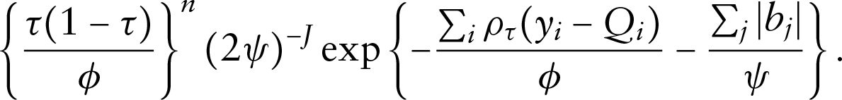
By using the simple re-parameterization ψ = ϕ λ and taking the log yields the log likelihood, apart from a constant,

ℓ = − n log ϕ − J log ϕ + J log λ − ∑ i ρ τ ( y i − Q i ) ϕ − λ ∑ j | b j | ϕ .

(3.1)

If ϕ and λ are considered as nuisance, then maximization of (3.1) with respect to the b j s justifies minimization of (2.2). Actually, (2.2) is more general as it includes multiple λ k and penalty on the differenced coefficients, however the rationale is clearly the same.

The partial derivatives of (3.1) are easily obtained

∂ ℓ ∂ λ = J λ − ∑ j | b j | ϕ ∂ ℓ ∂ ϕ = 1 ϕ 2 − ϕ ( n + J ) + ∑ i ρ τ ( y i − Q i ) + λ ∑ j | b j | .

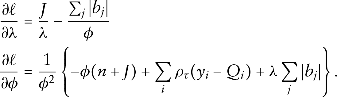
The root of ∂ ℓ ∂ λ = 0 is λ ̂ = ϕ ∑ j | b j | / J , while by the estimating equation ∂ ℓ ∂ ϕ = 0 , after plugging in λ ̂ , we get ϕ ̂ = ∑ i ρ τ ( y i − Q i ) / n . Namely the maximum likelihood (ML) estimate of scale parameters ratio λ is

λ ̂ = ∑ i ρ τ ( y i − Q ̂ i ) / n ∑ j | b ̂ j | / J = ϕ ̂ ψ ̂ ,

(3.2)

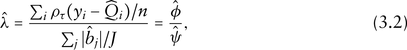
which justifies Step 4 in the aforementioned algorithm, apart from the denominators n and J . The rationale of replacing them with the effective degrees of freedom and details about their computation are discussed in the next subsections.

3.3 Quantifying the effective model dimension

The aforementioned algorithm in Step 3 requires to quantify the term-specific degrees of freedom edf k . To the best of our knowledge, there is no consensus in quantifying them for additive QR. Some criteria aimed at selecting the amount of smoothing, such as the CV (Bollaerts et al., 2006) or L -curve (Andriyana et al., 2014), do not need term-specific degrees of freedom, while other criteria, such as the Akaike or the Schwarz Information Criterions just require the overall effective model dimension. For instance in Koenker (2011), the multiple smoothing parameters in additive QR, are selected by

SIC λ = log n − 1 ∑ i n ρ τ ( y i − Q ̂ i ) + 0.5 n − 1 edf log ( n ) ,

(3.3)

where only the total edf are computed via the null residuals; see also Koenker (2005) for a general discussion, and Li and Zhu (2008) for a rigorous proof on computing the model complexity via the number of interpolated points. In a REML-like framework, the term specific edf k should clearly depend on the selected λ k , namely edf k = J k when λ k = 0 , and edf k → d k − 1 if λ k → ∞ . Two approaches could be undertaken to compute edf k at intermediate values of λ k .

The L 1 penalty leads to null estimates of some basis coefficients involved in the penalty term. Thus, a natural way to quantify complexity of the fitted curve is via the corresponding non-zero penalized estimates. More specifically, for the smooth term k expressed by a J k -rank basis and J k − d k penalized coefficient differences, we count the number of non-zero difference estimates and the number of underlying d k − 1 unpenalized coefficients; formally edf k = # { Δ d k b ̂ k ≠ 0 } + ( d k − 1 ) . For instance, if we set d k = 2 and λ k gets very large, we get all zero estimated differences, leading to edf k = d k − 1 = 1 which corresponds to the resulting linear fit.

The second viable approach relies on a smooth approximation of the L 1 norm in both the fidelity and penalty term. The goal is to build an approximate hat matrix in order to define the edf k s accordingly. Among the several smooth approximations which could be used (e.g., Muggeo et al., 2012), we use the simple identity | u | = u 2 / u 2 (Schnabel and Eilers, 2013). However, while Schnabel and Eilers (2013) use that to estimate multiple quantile curves with P-splines via iterative least squares, we exploit the smooth approximation only to build the hat matrix. Thus, given parameter estimates obtained via optimization of the L 1 -norm objective (2.2), residuals e i = y i − Q ̂ i and weights w τ i = τ − I ( e i < 0 ) arranged into the matrix W τ = diag ( w τ 1 , … , w τ n ) , we note the parameter estimates can be expressed via ( β ̂ , b ̂ λ ) T = ( X T W τ X + P λ ) − 1 X T W τ y , where X is the design matrix including linear covariates and the B-spline basis functions for the smooth terms and P λ is a block diagonal matrix including the zeroes for unpenalized coefficients and the penalty matrices relevant to the different smooth terms. For instance, the block relevant to the k th smooth term would be λ k D k d k T V k D k d k , where D k d k is the d k -order difference matrix and V k includes the reciprocals of the same differenced coefficients such that the quadratic form penalty equals the original L 1 -norm penalty, namely b k T D k T V k D k b k = ∑ j ( Δ d k b k ) j 2 ( Δ d k b k ) j 2 = ∑ j | Δ d k b k | j .

The least squares formulation allows to define the hat matrix whence the model degrees of freedom may be obtained. More specifically, the elements on the main diagonal of ( X T W τ X + P λ ) − 1 X T W τ X represent the degrees of freedom of each coefficient associated to the corresponding column of the design matrix. By summing the J k elements corresponding to the coefficients b k 1 , … , b kJ k relevant to the k th B-spline basis, the term-specific edf k are obtained. Of course, the trace quantifies the overall model edf .

We assess the performance of the proposed approach via some simulation experiments. We follow some settings employed in Koenker (2011), but we also consider additional scenarios. Data were generated according to y i = g ( x i ) + σ ( x i ) e i , where the covariate x i ∼ U ( 0 , 1 ) and the signal g ( x i ) is defined according to four different functions: linear 0.2 + 0.4 x i , logarithm log ( x i ) , sinusoidal sin ( 2 π x i ) and ‘square root sinusoidal’ indicated by g 0 ( x i ) = x i ( 1 − x i ) sin ( ( 2 π ( 1 + 2 − 7 / 5 ) ) / ( x i + 2 − 7 / 5 ) ) . The scale function is either constant σ ( x i ) = 0.2 or depending on the covariate itself, that is, σ ( x i ) = 0.2 ( 1 + x i ) . The errors e i are iid from four different distributions, Gaussian, χ 3 2 , t 3 and t 1 , such that the τ th quantile equals zero. The sample size is n = 400 and five percentiles τ = { 0.10 , 0.25 , 0.50 , 0.75 , 0.90 } are considered. To provide an idea of the signal to noise ratio in the considered scenarios, Figure 1 portrays a set of simulated data (at τ = 0.5 ) according to the different signal functions and error distributions.

OPEN IN VIEWER

Figure 1:

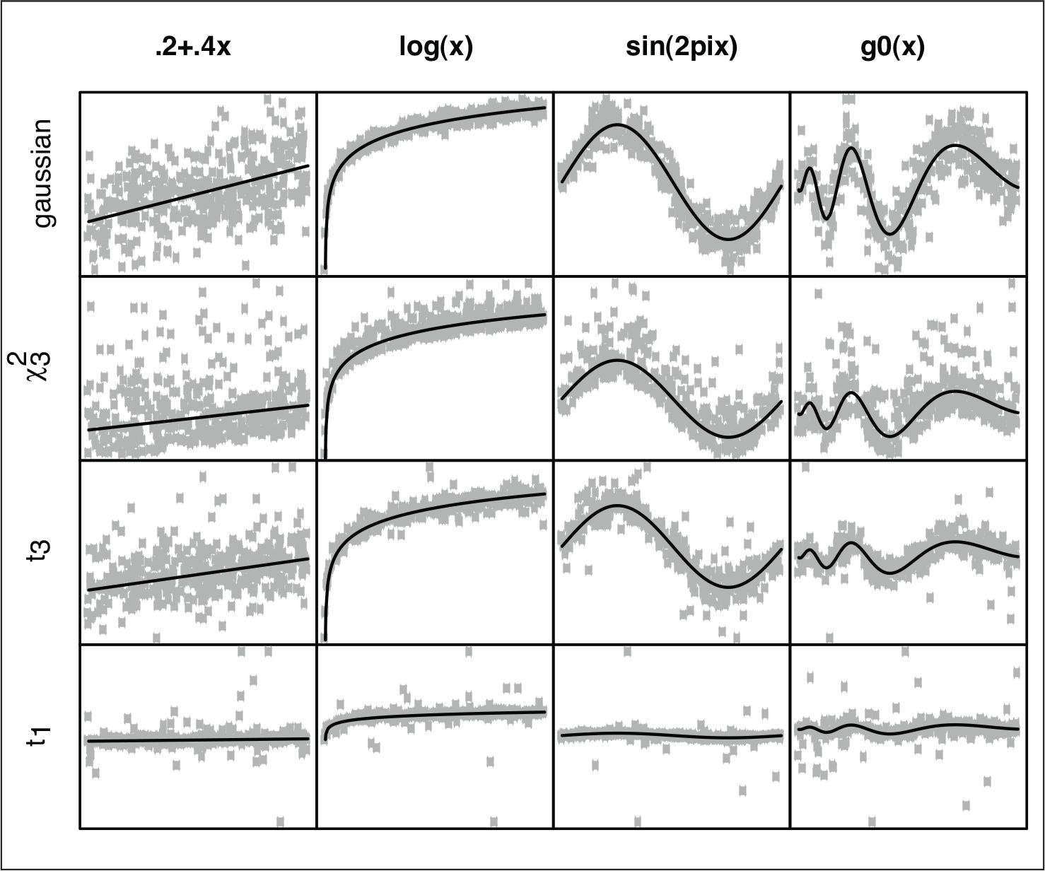
Some simulated data according to the signal curves and error distributions with constant scale function. The continuous line represents the true median signal

In the manuscript, we contrast three competitors: (a) the P-spline smoother (using min { 40 , n / 4 } cubic B-spline functions with difference penalty d = 3 ) and λ selected using the extra penalty factor γ = 2 in the Harville–Fellner–Schall Step 3 of the proposed algorithm (‘psplines+hfs’); (b) the same P-spline smoother with λ selected by the SIC λ reported in (3.3), (‘psplines + sic’); (c) the quantile smoothing splines with a total variation penalty and λ selected again by minimization of the SIC λ , (‘ssplines + sic’). Differences of the proposed ‘pspline+hfs’ with respect to other possible approaches, such as CV and the so-called L -curve criterion, are reported in Supplementary Material. Both CV and L -curve have been employed in literature to select just a single and not multiple, smoothing parameter in QR. Extension of tenfold, say, CV is prohibitive in practice due to its computational load, and L -curve for bivariate smoothing has been proposed in linear regression only (Frasso and Eilers, 2013), and further studies and research are needed to assess its applicability in additive QR (2.1). Therefore, both CV and L -curve could not be considered as effective competitors in additive QR, and discussion and comparative assessment has been reported in supplementary material which also includes some comparisons with the boosting approach.

OPEN IN VIEWER Figure 2:

Constant scale function σ ( x ) = 0.2 . Contrasting three competitors for smoothing parameter selection in terms of MISE (on log scale) by different error distributions and signals: ‘sspline+sic’ (light grey box), ‘pspline+sic’ (medium grey box) and ‘pspline+hfs’ (dark grey box)

OPEN IN VIEWER Figure 3:

Non-constant scale function σ ( x ) = 0.2 ( 1 + x ) . Contrasting three competitors for smoothing parameter selection in terms of MISE (on log scale) by different error distributions and signals: ‘sspline+sic’ (light grey box), ‘pspline+sic’ (medium grey box) and ‘pspline+hfs’ (dark grey box)

The three aforementioned main approaches are contrasted in terms of Mean Integrated Square Error (MISE) defined as the mean of squared differences between the true quantile curve and the corresponding fitted curve across 500 replicates, and also the Mean Integrated Absolute Error, similar to MISE but involving the absolute differences rather than the squares. Here we report results for the MISE values, while the MIAE results are reported in the Supplementary Material.

Figures 2 and 3 report the comparisons in terms of MISE: for all the error distributions considered and for every signal (linear, logarithmic, sinusoidal and sqrt+sinusoidal ‘ g 0 ( · ) ’), each panel reports the boxplots of the log MISE values across the replicates for the five τ values. The two figures refer to homoscedastic and heroscedastic scenarios.

Overall, no important difference emerges across the scenarios. Occasionally, some criterion appears to perform slightly better/worse than the others: for instance, ‘sspline+sic’ returns higher MISE values at higher quantiles with log ( x ) signal and gaussian errors; the proposed ‘pspline+hfs’ exhibits slightly lower mean square errors at linear signal and middle percentiles (0.25,0.50,0.75), but at the same middle percentiles, it depicts higher values when the signal is log ( x ) or g 0 ( x ) and errors follow the Cauchy distribution. However, no systematic patterns come out, and no difference among the homoscedastic or heteroscedastic case is noteworthy. Hence, while performances in terms of statistical efficiency are substantially the same across the scenarios, the gain in computational efficiency is not negligible; more details are postponed to Section 4.1.

The same simulation scenarios were run with an additional linear covariate to assess possible impacts on the sampling distribution of the linear coefficient estimators. No difference was observed among the MISE values and the sampling distributions and results are not shown for shortness.

We consider the more interesting scenarios of additive models, namely more smooth relationships in the QR equation. To illustrate, we consider the true quantile function 1 + 2 cos ( x 1 i ) + sin ( 2 π x 2 i ) with independent uniform covariates x 1 i ∼ U ( − 4 , 4 ) and x 2 i ∼ U ( 0 , 1 ) , sample size n = 400 , the four aforementioned error distributions and five quantile curves. Figure 4 shows the log MISE, for the aforementioned competitors ‘sspline+sic’, ‘pspline+sic’ and the proposed ‘pspline+hfs’.

OPEN IN VIEWER Figure 4:

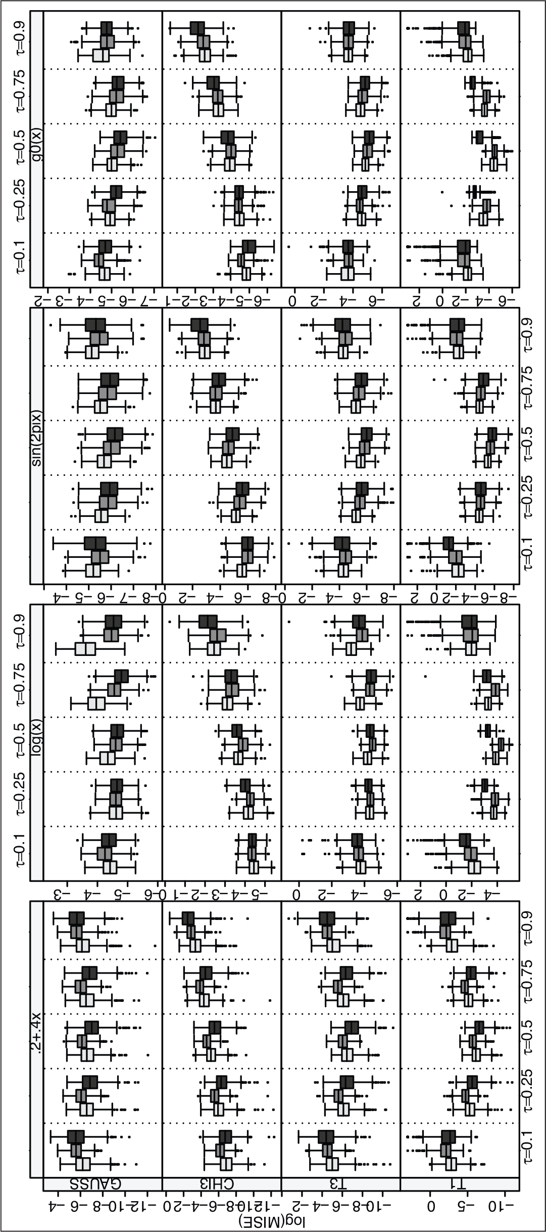
Contrasting the three competitors (in terms of log(MISE)) for smoothing parameter selection with 2 additive terms by different error distributions and quantile curves: “sspline+sic” (light grey box), “pspline+sic” (medium grey box) and “pspline+hfs” (dark grey box). Right panels: constant scale function; left panels: non-constant scale function. The true signal is 1 + 2 cos ( x 1 i ) + sin ( 2 π x 2 i )

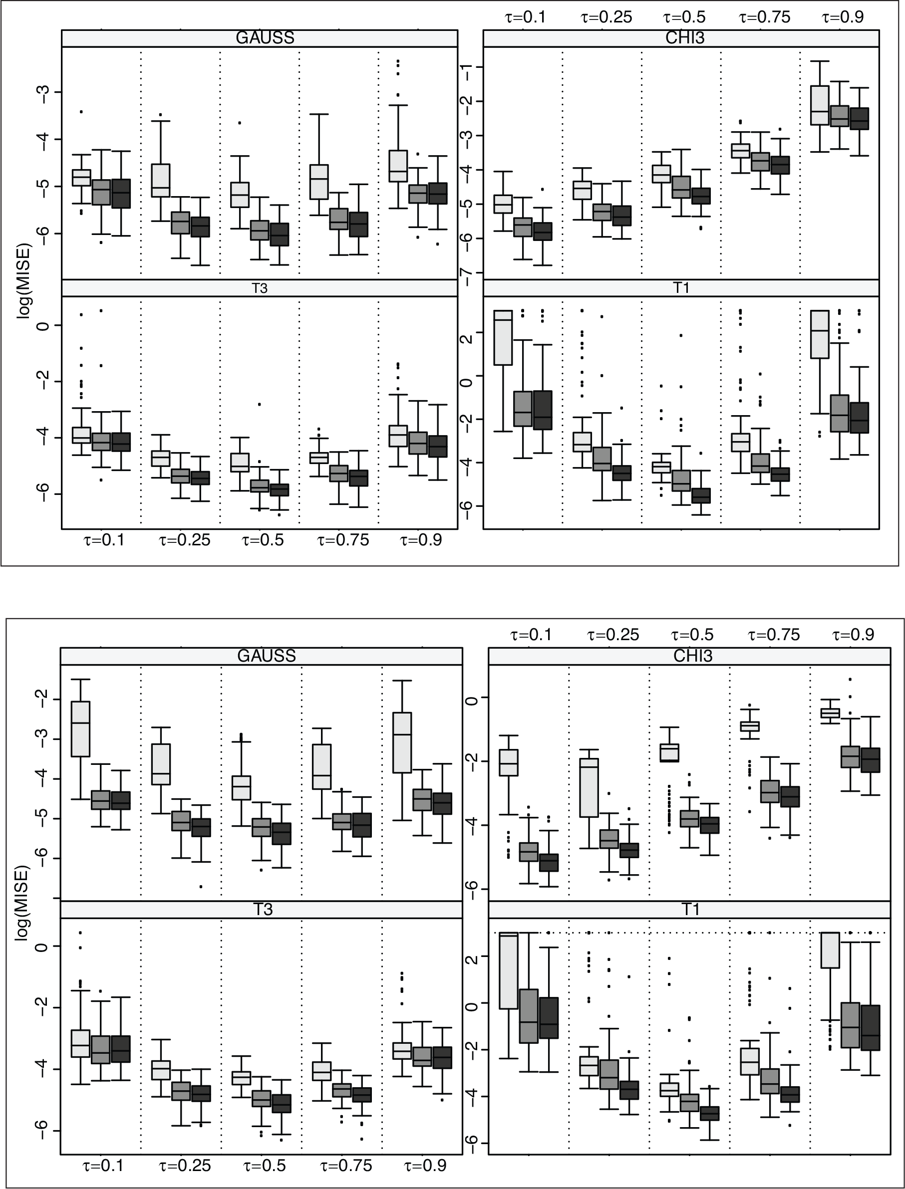
Unlike the single covariate case, here some differences are noteworthy. For the homoscedastic scenario, the traditional ‘sspline+sic’ performs bad most of times, noticeably quite worse than the others with Gaussian and Cauchy errors especially at extreme quantiles ( τ = 0.1 and 0.90 ). On the other hand, ‘pspline+sic’ and ‘pspline+hfs’ behave about the same, with ‘pspline+hfs’ exhibiting lightly but constantly lower MISE values at middle quantiles ( τ = 0.25 , 0.50 , 0.75 ) with somewhat remarkable differences in the t 1 -distribution case. With heteroscedastic errors patterns are even more pronounced, especially with asymmetric errors where the MISE values from ‘sspline+sic’ are far higher than the others.

Differences in terms of MISE exhibit approximately the same patterns and are reported in the supplementary material which also shows comparisons relevant to smoothing parameter selection in varying coefficient models.

4.1 Computational issues

As previously discussed, computational efficiency is a major feature of our proposal. The benefit with respect to crude grid search approaches could be somewhat expected, especially when multiple smoothing parameters have to be estimated: in fact grid-search approaches require multidimensional evaluation grids leading to quite taxing procedures since a large number of fits have to be obtained to pick up the best lambdas values optimizing the selected criterion, such as the SIC or L -curve. CV is even heavier, since for each candidate lambda value in the grid, the model has to be fitted and tested several times to training/testing sub-datasets.

OPEN IN VIEWER

Table 1:

Computational times to fit additive quantile regresion with 1 or 2 smooth terms for n = 1 000 observations. Entries refer to averages (on 10 fits) of the elapsed components obtained via the system.time() function in R. Times also include building the B-spline basis and the penalty matrices. Computations run on R 3.6.1 on Windows, Intel i7-8700 CPU 3.20 GHz, RAM 16 GB.

N. Smooth				Execution
Terms	Criterion	Method		Time (Sec.)
1	sspline+sic	grid-search ( 15 )		0.12
		grid-search ( 30 )		0.21
	pspline+sic	grid-search ( 15 )		0.12
		grid-search ( 30 )		0.22
	pspline+hfs	iterative		0.07
2	sspline+sic	grid-search ( 15 × 15 )		57.3
		grid-search ( 30 × 30 )		228.7
	pspline+sic	grid-search ( 15 × 15 )		8.61
		grid-search ( 30 × 30 )		33.1
	pspline+hfs	iterative		0.33

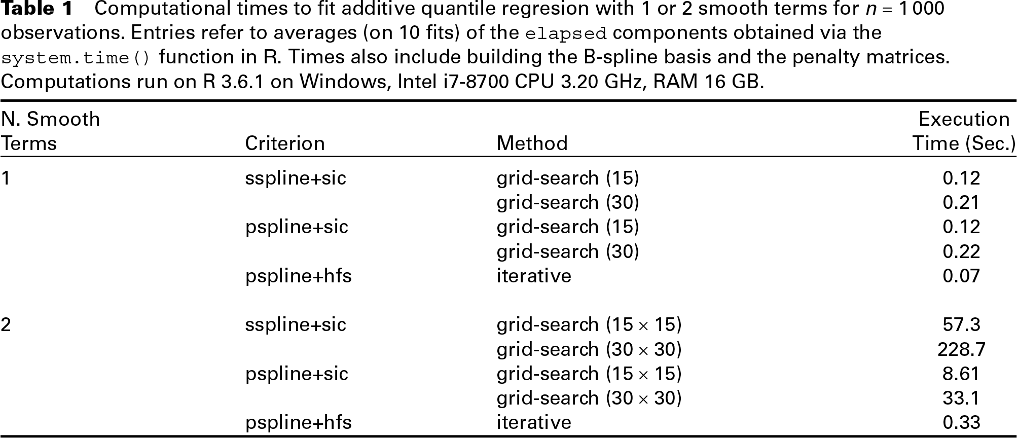
To gain a rough assessment of the computational load, Table 1 reports the execution time of the aforementioned approaches when fitting additive regression quantiles with 1 or 2 smooth terms at τ = 0.5 for n = 1 000 observations. For the ‘grid-search’ rows, the numbers in parentheses refer to the number of lambda values to be evaluated to seek the optimum: We consider 15 or 30 values, with the former leading, as it would be expected, to lower execution times but higher mean square errrors.

While for single smooth terms, all times are within reasonable ranges, differences get notable with 2 smooth terms: grid-searches show quite large times in general, but sspline+sic exhibits larger running times, probably due to the higher number of parameters to be estimated. The proposed pspline+hfs presents times far lower than the competitors, since it is based on iterative procedure and typically less than 20 iterations are requested to get convergence. It is worth stressing that such large differences are expected to rise as the number of smoothing parameters increases, making our proposal quite attractive with multiple additive terms.

For the sake of completeness, we mention the SIC criterion could be minimized via numerical procedures rather than grid-searches: For instance, by means of the Nelder–Mead algorithm which does not require gradient evaluation, or quasi-Newton methods which compute the gradient numerically. However, we have experienced a somewhat strong influence of the supplied starting values on the final results, making the numerical procedures substantially unreliable. One could try to run the algorithm using different starting values or probably to rely on different algorithms such as the simulated annealing, but at the cost of increasing the computational burden.

We apply the proposed algorithm to analyse data concerning the sport performance in children. Physical fitness is a powerful marker of the health condition in childhood and adolescence; for instance, fitness is negatively associated with cardiovascular risk factors for chronic disease, high blood pressure and total fatness (Kraemer and Häkkinen, 2008).

As an alternative to laboratory methods, physical fitness can be measured via the on-site fitness tests which are easy to be administered, especially when the population study involves schoolchildren. Among the different sport performance outcomes, the standing long jump (SLJ) test represents a widespread yet practical, time-efficient and cheap method for assessing the muscular fitness in children and adolescents. The schoolchildren stands at a line marked on the ground with the feet slightly apart and jumps: The SLJ performance is the horizontal distance jumped. SLJ, sometimes also known as standing broad jump, is commonly used to assess explosive leg power, but it is is also understood to be a proxy of muscular strength tests of the lower body. SLJ depends mainly on leg length, but it influenced also by neuromuscular maturation, as SLJ requires more coordination of movements and technique, for instance the so-called take-off angle (Saint-Maurice et al., 2015).

Data analysed here refer to wide survey carried out in years 2011–2013 to assess sport abilities and fitness in schoolchildren in Sicily. Data have been kindly provided by the Department of ‘Scienze Psicologiche, Pedagogiche e della Formazione’, University of Palermo. Measurements were gained by previously trained experts and include measurements on performance on several physical tests along with some anthropometric measurements collected in the major Sicilian cities in the three-year period. Here we present results relevant to n = 488 schoolchildren in Palermo collected in 2011; further results relevant to whole Sicily will be presented elsewhere.

Beside the response SLJ, the main covariate is the child weight. The substantive research question is how the weight could affect the SLJ performance, namely in statistical terms the relationship SLJ—weight which is expected to be nonlinear. However, the weight is strongly correlated with age and height, which are understood to affect the response as well, possibly in a nonlinear manner. Thus, an additive QR accounting simultaneously for the three covariates flexibly appears to be the most appropriate model, namely

Q slj ( τ ) = β 0 + β 1 gender + s 1 τ ( age ) + s 2 τ ( weight ) + s 3 τ ( height ) ,

at fixed τ . Multiple quantile curves could be useful to obtain the so-called growth charts, sometimes referred to as ‘normative reference values’ in sport medicine (Saint-Maurice et al., 2015; Sandercock et al., 2016). However, focusing only on upper quantiles would be useful for talent selection in school age. Thus, we set τ = 0.95 in the above regression equation.

We fit the additive QR model using the aforementioned algorithm; the smooth functions are expressed as identifiable cubic B-spline bases and the number of basis functions was set using the empirical rule of min { 40 , n / 4 } (Ruppert et al., 2003). A third-order difference penalty was used in the penalty term.

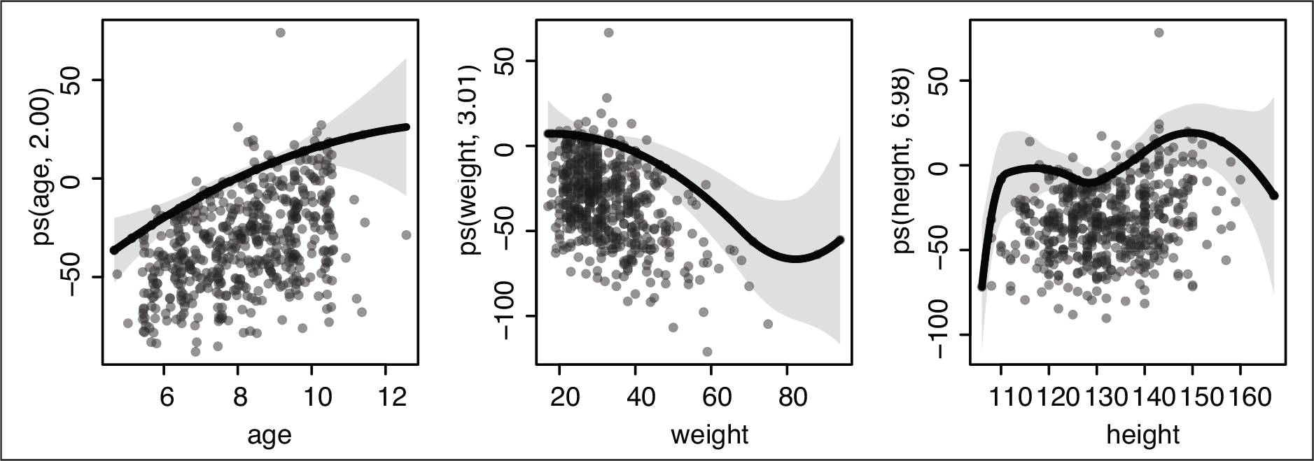
Figure 5 portrays the fitted curves (centred due to identifiability constraints) along partial residuals, that is, the fitted quantile values plus the residuals from the full model. To quantify uncertainty, pointwise confidence intervals have been computed by means of the estimates covariance matrix based on bootstrap cases resampling.

OPEN IN VIEWER

Figure 5:

The smooth effect of age, weight and height on the quantile curve τ = 0.95 of standing long jump. In each panel, shaded areas portray the 95% pointwise confidence intervals based on bootstrap resampling and dots represent the partial residuals

For the age term, the smoothing parameter estimate is quite large, and thus the relevant relationship with the response corresponds to a polynomial of degree 2; on the other hand, the estimated lambdas for the weight and height terms are moderate, resulting in flexible relationships with 3.01 and 6.98 degrees of freedom, respectively. Controlling for age and height, the weight effect on the SLJ is worth discussing: Until 35–40 kg, there is almost no influence on the performance, but afterwards there is an important negative effect untill about 75 kg when the relationship stabilizes. Finally, the height effect shows different phases, with steeper slopes at very low ( < 110 cm) and at middle (130–150 cm) heights.

We have discussed estimation at single specified τ . However, if the aim is to estimate multiple quantile curves at different τ values, the proposed algorithm could be applied several times at different τ values with the noncrossing constraints as discussed in Muggeo et al. (2013).

We have proposed an iterative algorithm for selecting multiple smoothing parameters in additive QR models with L 1 penalties. The idea exploits the link between smoothing and mixed modelling, a connection which is well consolidated in mean regression, but it appears not fully exploited in QR. The iterative nature of the proposed algorithm makes it very attractive in presence of several lambdas where the multidimensional grid search or the derivative-free numerical optimization demand extensive computations. While the algorithm relies on assuming proper Laplace distributions for the responses and the random effects with constant scale parameters, simulations have shown that our approach performs well even when the constant-scale assumption is violated and observations exhibit heteroscedasticity. This is quite remarkable from a practical perspective, since QR turns out to be very useful especially in heteroscedastic scenarios.

In addition to far better computational efficiency, simulation experiments have shown that most of the times our proposal exhibits good statistical performance as compared to the canonical approaches of smoothing splines or P-splines and tuning parameter selected by the Schwartz Information Criterion. The proposed approach returned slightly higher mean squared errors only in few scenarios at the lowest quantile ( τ = 0.1 ). Along with the algorithm itself, we have also discussed a strategy to quantify the equivalent degrees of freedom of the fitted model and also of each smooth term. In additive QR, quantification of the equivalent degrees of freedom for each smooth term does not appear to have been discussed previously.

We have focused on additive models, that is, multiple ‘univariate’ smooth terms, but generalization to bivariate smooths represents straightforward extensions where our proposal could apply. Modelling multiple quantile curves to produce growth charts for reference values can be carried out by applying the proposed algorithm at different probability values, namely with τ -specific smoothing parameter values. As an alternative option, a unique smoothing parameter could be used for each quantile curve: Selecting and using a unique smoothing parameter for each τ value represents a noteworthy issue to be investigated.

Also, the presented algorithm could be employed in random effects QR for longitudinal data, where a few proposals have been discussed (Koenker, 2004; Geraci and Bottai, 2007; Lamarche, 2010): Comparisons with Geraci and Bottai (2007) which use explicit marginal Laplace log likelihood and Gibbs sampler appear particularly noteworthy.

Yet another possible extension of the proposed algorithm is about modelling quantiles from discrete distributions, for instance to study the student performance at university via the number of credits gained after the first academic year (Grilli et al., 2016): Here QR is applied several times at the randomly jittered response, and if the smoothing parameter has to be estimated at each perturbated dataset, the proposed approach appears quite useful due to computational efficiency.

R code to implement the methods presented in this article is currently available from the corresponding author and will be also shipped in due time with the R package quantregGrowth. Detailed comparisons among the R packages to fit additive regression quantiles represent a noteworthy point to be investigated in a separate paper.

Supplementary materials

Supplementary materials for this article, including comparisons with other approaches along with further simulation results, R code and data discussed in Section 5, are available from http://www.statmod.org/smij/archive.html