



Abstract
This article develops an approximate N-mixture model for infectious disease counts that accounts for under-reporting as well as spatial dependence induced by person-to-person spread of disease. We employ the model to estimate actual case counts in Oregon of chlamydia, an easily-treated but usually asymptomatic sexually transmitted disease. We describe a combined parametric bootstrap to account for uncertainty in parameter estimates as well as sampling variability in actual case counts. A simulation study illustrates that our method performs well in many scenarios when the model is correctly specified, and also gives reasonable results when the model is misspecified, and no spatial dependence exists.
Introduction
Estimating the true prevalence of under-reported or under-ascertained diseases is difficult to accomplish without knowledge of local demographics or extensive studies (Gibbons et al.(2014) Gibbons, Mangen, Plass, Havelaar, Brooke, Kramarz, Peterson, Stuurman, Cassini, Fèvre, et al.). Additionally, understanding the dynamics of a disease is an important step in understanding changes in prevalence over time (Ostfeld et al.(2005) Ostfeld, Glass, and Keesing). With certain diseases, such as infectious diseases, we would expect there to be spatial dependence among the prevalence of diseases at locations near each other. We aim to provide a spatially explicit statistical method for surveilling imperfectly detected diseases using the reportable disease infrastructure already established through the Centers for Disease Control and the Oregon State Health Authority.
(Brintz et al.(2018) Brintz, Fuentes, and Madsen) established the use of the asymptotic N-mixture model as an appropriate model to make disease prevalence estimates for high-abundance imperfectly-detected or under-reported diseases but disregarded any spatial dependence of the disease prevalence. Other extensions of the N-mixture model have used factors such as weather, habitat, density dependence, to account for spatial patterns (Rossman et al.(2016) Rossman, Yackulic, Saunders, Reid, Davis, and Zipkin). In (Zhao et al.(2017) Zhao, Royle, and Boomer), we see the first spatially explicit N-mixture model which models survival, reproduction, emigration, and abundance while representing movement among adjacent habitat patches. They model the spatial relationship using an immigration random variable, suggesting that the number of immigrants to site
Our spatial model employs a neighbourhood structure to account for the spread of disease between adjacent sites, whereas the model of (Brintz et al.(2018) Brintz, Fuentes, and Madsen) had no mechanism to capture the spatial pattern of infection. As a further advancement, we augment the parametric bootstrapped confidence intervals to account for sampling variation in disease counts as well as uncertainty in the model's parameter estimates.
This article is organized as follows. Section 2 presents the Oregon chlamydia data which we use as a motivating example and subsequently analyse in Section 7. Section 3 briefly describes N-mixture models in general and an estimability diagnostic. The proposed spatial asymptotic N-mixture model is described in Section 4. In Section 5, we compare the spatial model to the non-spatial asymptotic model using the diagnostic given in Section 3. In Section 6, we use simulated data with spatial covariance to test the new model's performance and also compare its performance to a model without spatial covariance information. In Section 7, we include an analysis of the chlamydia data using the new spatial model. Section 8 gives some concluding remarks.
The chlamydia data
Chlamydia is a sexually transmitted infection caused by the bacterium Chlamydia trachomatis. Chlamydia is imperfectly detected because most people who have it do not have symptoms. Since the infection can be cured if detected, a statistical model should allow for the reduction of cases over time. The infectious nature suggests that neighbouring population centres may have similar prevalence, so a model that accounts for spatial dependence and allows an increase in cases through sexual transmission is appropriate. (Brintz et al.(2018) Brintz, Fuentes, and Madsen) analysed chlamydia data for 2007–2016 obtained from the Oregon Health Authority (
Table 1 illustrates the structure of the data, which includes annual population estimates and observed counts of reported chlamydia cases. The observed chlamydia counts of the most populous counties are two to three orders of magnitude larger than those of the least populous counties.
The chlamydia data includes yearly population estimates and observed disease cases for all 36 of Oregon's counties. The table shows data for the five most populous and the five least populous counties

The chlamydia data includes yearly population estimates and observed disease cases for all 36 of Oregon's counties. The table shows data for the five most populous and the five least populous counties
A heat map of the 2016 reported chlamydia prevalence in all Oregon counties
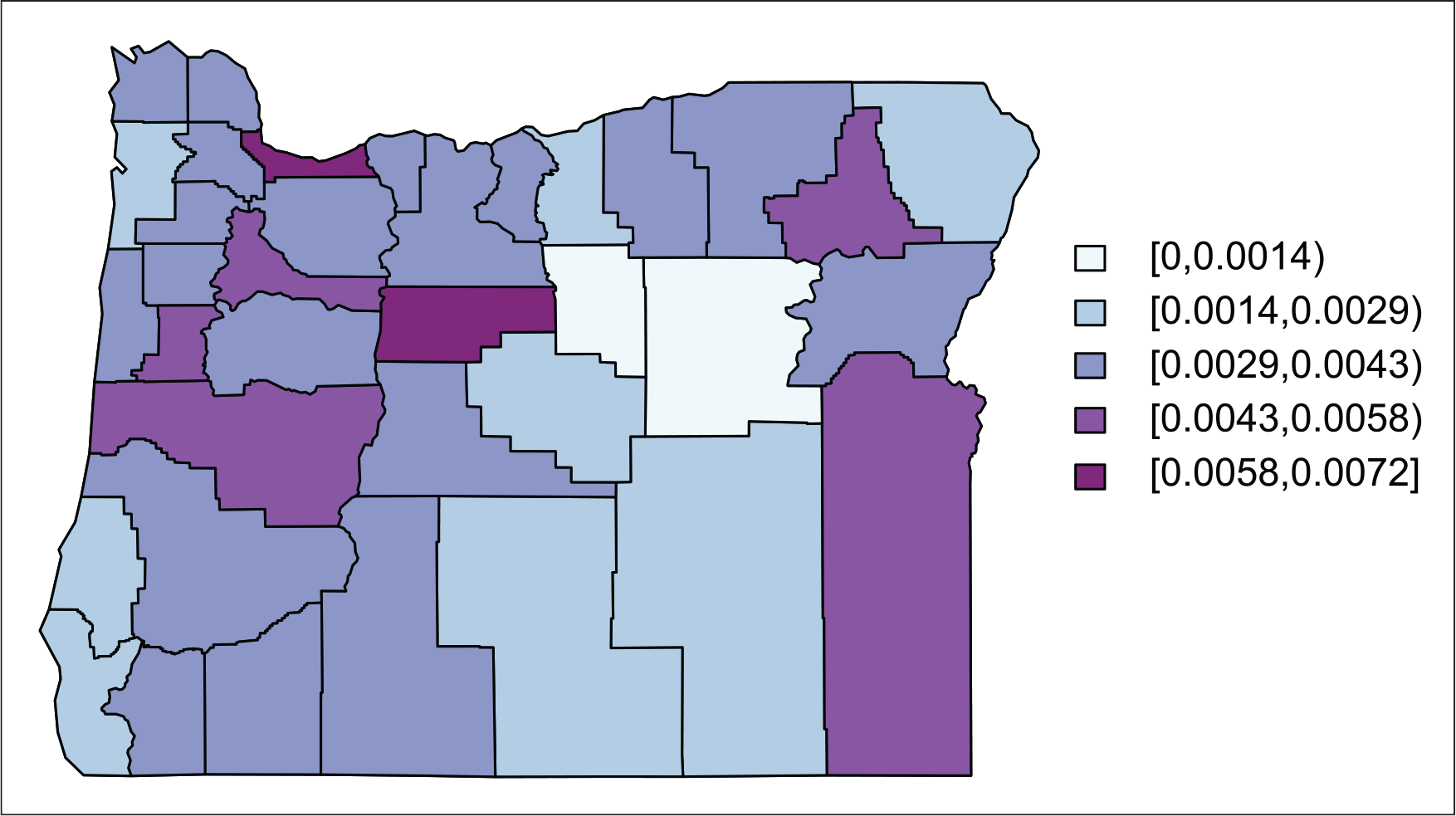
Figure 1 shows a map of Oregon's 36 counties, shaded by reported chlamydia prevalence in 2016, and suggests spatial dependence, since counties close to each other have similar prevalence. We will utilize county prevalence in the spatial component of our proposed model.
(Royle (2004)) introduced N-mixture models for estimating the size 
with 
where
(Dail and Madsen (2011)) relaxed the population closure assumption. The goal of their model was to estimate 
with 

and as in (Royle (2004)), approximation of the summations to infinity are made using a large finite
(Brintz et al.(2018) Brintz, Fuentes, and Madsen) adapted the generalized N-mixture model to model counts of disease cases, using the Oregon chlamydia data for 2007–2016 mentioned Section 2 as a case study. The chlamydia data includes several observed counts exceeding 1 000, much too large for the generalized N-mixture model. Therefore, they proposed a multivariate normal (MVN) approximation of the generalized N-mixture likelihood (3.2) based on a normal approximation to the binomial and to the Poisson, thus avoiding the infinite sums.
The sites are assumed to be independent, so the MVN approximated likelihood is

where MVN (⋅,⋅) denotes the multivariate normal density function, μi is the T × 1 mean vector for site i, and Σt is the T × T covariance matrix for site i. Parameter vector θ includes parameters for the distribution of initial prevalence Ni1/popi, where
In addition to avoiding the infinite sums of (3.2), the MVN approximation (3.4) has a closed-form expression for the Fisher information matrix
The asymptotic N-mixture model of (3.4) assumes independence between sites, so the observed data vector
Our focus is on estimating disease prevalence, so we now assume that, as is typical in disease surveillance, observations exist for all sites at all time periods within the scope of the study. In the chlamydia data, the sites are Oregon's counties, and the time periods are the years from 2010 to 2018. In this context,
Given that parameter identifiability is a general concern with N-mixture models, we model spatial dependence without including extra parameters that might be confounded with parameters from the non-spatial components of the model. In order to accomplish this, we incorporate spatial dependence based on adjacency, much like the conditional auto-regressive (CAR) model of (Abellan et al.(2008) Abellan, Richardson, and Best).
In particular, we construct an
For sexually transmitted diseases such as chlamydia, an adjacency matrix defined in this way is sensible because of the connection between the disease and the sex trade. Our model does not specify how adjacency is defined, so other criteria may be used to define an appropriate neighbourhood structure for other diseases.
Preliminary modelling attempts of the chlamydia data suggested that using an equal weighted neighbourhood was not appropriate due to the possibility of adjacent counties having very different population sizes. With equal weighting, the prevalence in very large or small populations disproportionately affects their neighbours. Therefore, we adjust our model to use a weighted prevalence model as described below.
As above
Components of the spatial model are



where
The recruitment process (cf. equation (3.3)) will now incorporate the previous time period's prevalence of all of site 
where

for
For simplicity, our implementation of the model assumes no spatial dependence within the first time period. The model could be augmented to include an initial spatial dependence structure, but here we focus on the spatial dependence induced by disease transmission and movement of infected individuals after a baseline time point.
Modelling
Our model also assumes negligible ‘edge effects’, that is, we suppose that Oregon's counties bordering other states are relatively unaffected by their out-of-state neighbours. In practice, one could include population and prevalence data from these neighbours in the analysis.
To complete the specification of the spatial model, we specify the conditional distribution of 
In order to implement this model, we approximate the joint likelihood of the observed data 
If 
where
To write the mean parameter 
by the law of total expectation and equations (4.1) and (4.1). For 
where
By ordering the
Because the
We define the
For 
For 
For 
Finally, for a diagonal element of 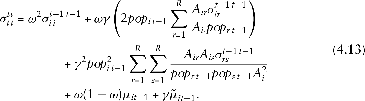
The resulting mean vector and covariance matrix are of the form

Equations (4.7) through (4.11), give the parameters of the approximate likelihood (4.6) in terms of parameter
We obtain yearly estimates of total cases using the approach in (Dail and Madsen (2011)) as follows. We estimate 


where
We determine approximate 95% confidence intervals for the
Similarly, we approximate the sampling distribution of the
We now compare the spatial model with the non-spatial using the Fisher information-based diagnostic described in Section 3. The asymptotic variance-covariance matrix of the the MLE of
The 
where
One improvement of the spatial model over the non-spatial model is that the
It should be noted that (5.1) is based on the true parameters. If parameter confounding occurs for a particular dataset, it will be difficult to obtain parameter estimates to substitute into (5.1). It may be possible to instead use historical information to set bounds for the parameters, then investigate identifiability from (5.1) by examining a limited number of plausible combinations of parameter values.
We conducted two simulation studies. The first explores the performance of the spatially explicit model, and the second investigates its robustness compared to the non-spatial model. In the first study, we used the Oregon adjacency matrix and county populations for the nine years 2010 to 2018 (Table 1) to simulate abundance data from 24 scenarios constructed using
We generated 1 000 simulated datasets for each scenario. For each simulated dataset, we optimized the log of approximate likelihood (4.6) with respect to
We calculated the absolute relative error of the prevalence estimates for county 
where 
We calculated a 90% confidence interval for
Each row is based on the successful simulations out of an attempted 1 000 simulated datasets using the given
,
,
and
values. ARE is the summarized absolute relative error from equation (6.2) averaged over the simulations, Cov% is the proportion of 90% confidence intervals for
that included the true value, and Width is the average width of these confidence intervals.
is the number of simulations out of 1 000 that successfully converged to a value properly inside the box constraints
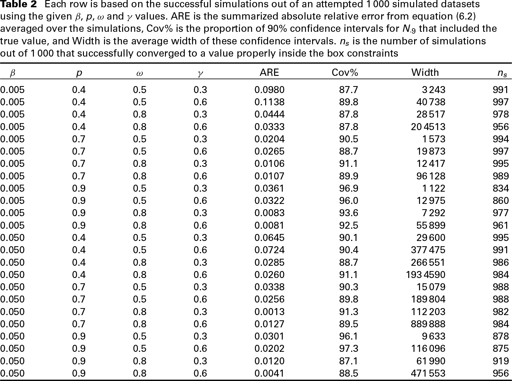
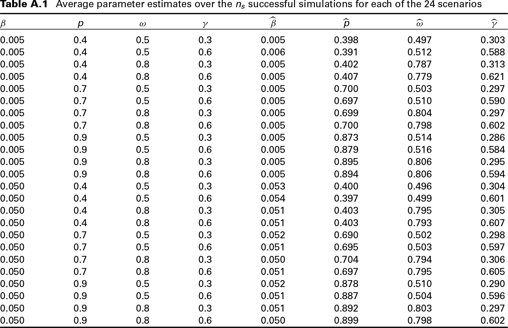
Table A.1 in the Appendix gives estimates of the four parameters
Table 2 shows simulation results for the abundance estimates. ARE is the summarized absolute relative error (6.2), averaged over the
Turning to confidence interval success percentage, we note that the nominal 90% coverage was no less than 87.1%. When
Average confidence interval widths were larger for higher settings of initial prevalence
The number of successful simulations out of the 1 000 attempted is at least 834, and usually over 950. The lowest values of
The second simulation study explored the same parameter settings but simulated data from the spatial model described in Section 4 as well as from the non-spatial model N-mixture model given in Section 3. Both models were fit to both types of simulations to explore robustness to model misspecification. We simulated 1 000 datasets for each simulation type and combination of parameters.
Each row is based on simulated data with
sites and
time periods using the given
,
,
, and
values. The two columns labelled Spatial Data represent 1 000 datasets simulated under the spatial model described in 4. The two columns labelled Non-spatial Data represent 1 000 datasets simulated under the generalized non-spatial M-mixture model of 3. Both the spatial model and the non-spatial model are fit to each dataset, and the ARE (6.2) is recorded. Omitted from the table are 10 scenarios where there were fewer than 750 successful optimizations out of 1 000 for any one of the four model fits

Table 3 gives results of the robustness simulations for the 14 scenarios where all four of the model fits involved more than 750 successful optimizations out of the 1 000 attempted. The ARE (6.2) using the correct model is smaller than the ARE from the misspecified model in all scenarios except one. The exception occurs when
We fit the chlamydia data to the spatially explicit model. Point estimates, asymptotic variances, and approximate 95% confidence intervals are shown in Table 4.
Output of R's optim function. MLE are the estimates,
are the diagonal elements of the inverse of the asymptotic information matrix evaluated at the MLE. Approximate 95% confidence limits (CL) are calculated as
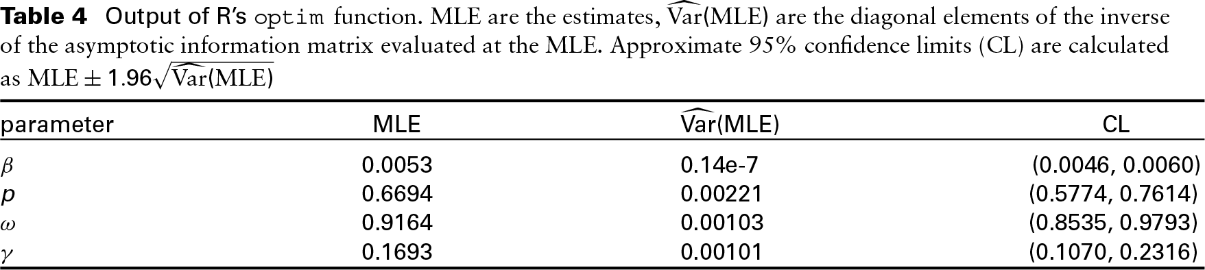
Output of R's optim function. MLE are the estimates,
are the diagonal elements of the inverse of the asymptotic information matrix evaluated at the MLE. Approximate 95% confidence limits (CL) are calculated as
The estimated initial prevalence was
Both observed total counts
and estimated total counts
of Chlamydia in Oregon for 2010–2018. Vertical bars represent 95% confidence intervals. The graph includes predicted total counts and 95% prediction interval for 2019
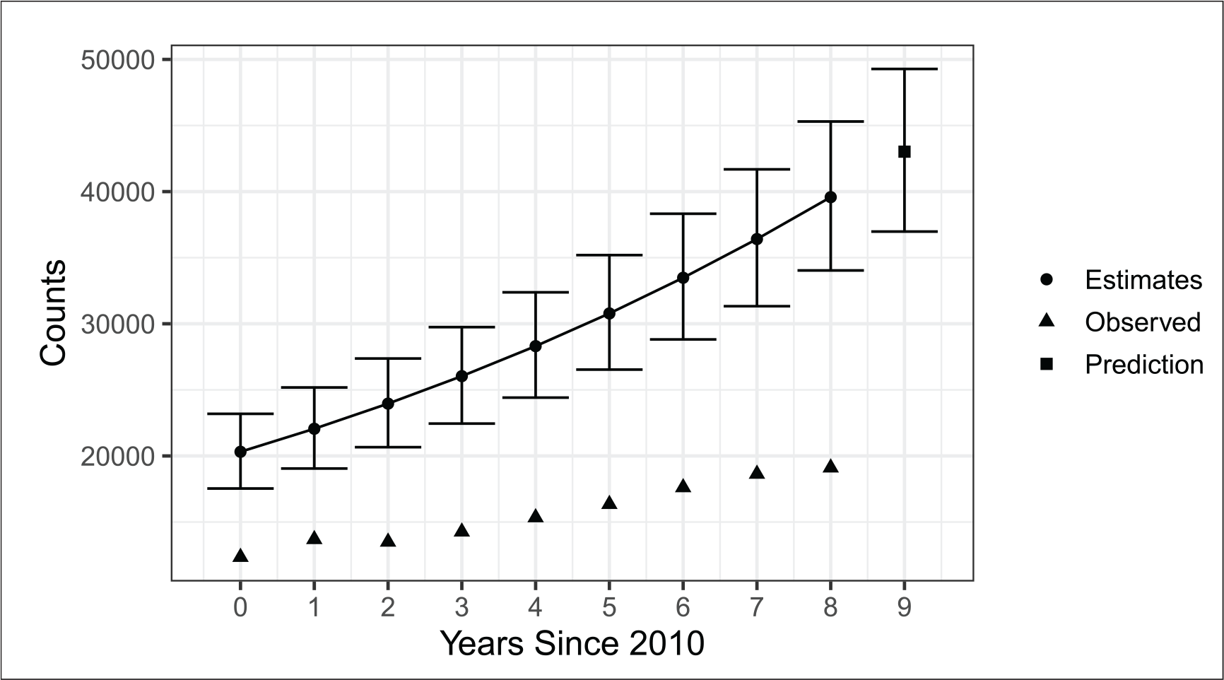
Figure 2 illustrates observed total counts
Figure 2 shows a steeper increasing trend of chlamydia cases than was found with the non-spatial model and similar precision in the confidence intervals. However, the confidence intervals shown here estimate
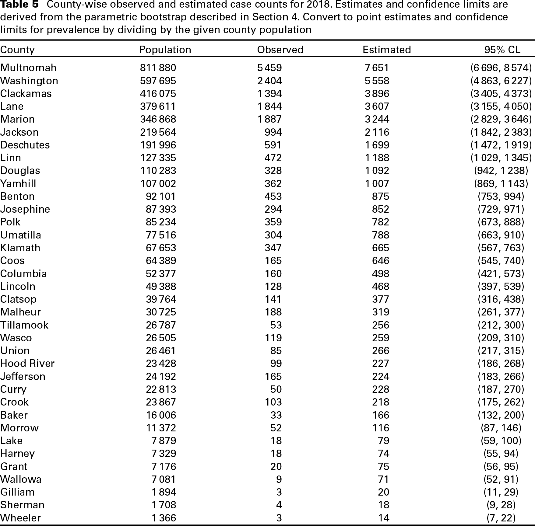
Instead of estimating state-wide totals, we can report county estimates
County-wise observed and estimated case counts for 2018. Estimates and confidence limits are derived from the parametric bootstrap described in Section 4. Convert to point estimates and confidence limits for prevalence by dividing by the given county population
We have developed a spatial extension to the asymptotic N-mixture model as a natural next step for modelling infectious disease data. The human to human connection suggests that a high prevalence in one location could encourage a high prevalence in neighbouring locations. As such, we induced the spatial dependence using a neighbourhood model. By basing the spatial dependence on prevalence by population rather than total case count over a year, we avoid letting highly populous counties disproportionately affect their more sparsely populated neighbours. The model assumes that the recruitment of cases into one county is based on the average prevalence of its neighbours (including itself) at previous time period. In contrast, the non-spatial model only conditions case recruitment on each county's own previous time period's prevalence.
We have shown through simulation that the spatial asymptotic approximation of the N-mixture model performs well in common scenarios and outperforms the non-spatial asymptotic approximation model with spatially dependent data. The
In the Oregon Health Authority chlamydia data, we see somewhat similar parameter point estimates between the spatial and non-spatial models for both the initial prevalence parameter
Future refinements of the spatial model include modelling the four parameters as functions of covariates, though we note that these must be at the same spatial scale as the observed counts. We may also consider redefining spatial adjacency so to better model the spatial pattern of infection. For example, in Oregon, there is more movement from north to south along the Interstate 5 corridor than there is in the east-west direction. This anisotropy could be modelled by extending neighbourhoods in the north-south direction.
Computing
The simulations and data analysis described in Sections 6 and 7 are coded in R (R Core Team (2016)). Source code and the Oregon chlamydia data are available at
Appendix
Details of covariance calculations of the MVN model
We define the
In all cases, we calculate cov (Nit,Nju) using the law of total covariance by conditioning on 
If 
which is why we have to consider the fourth case.
Case 1: Suppose
The diagonal elements 
Case 2: Suppose

The first term on the right-hand side of the first line of (A.3) is 0 because
Case 3: Suppose
Let 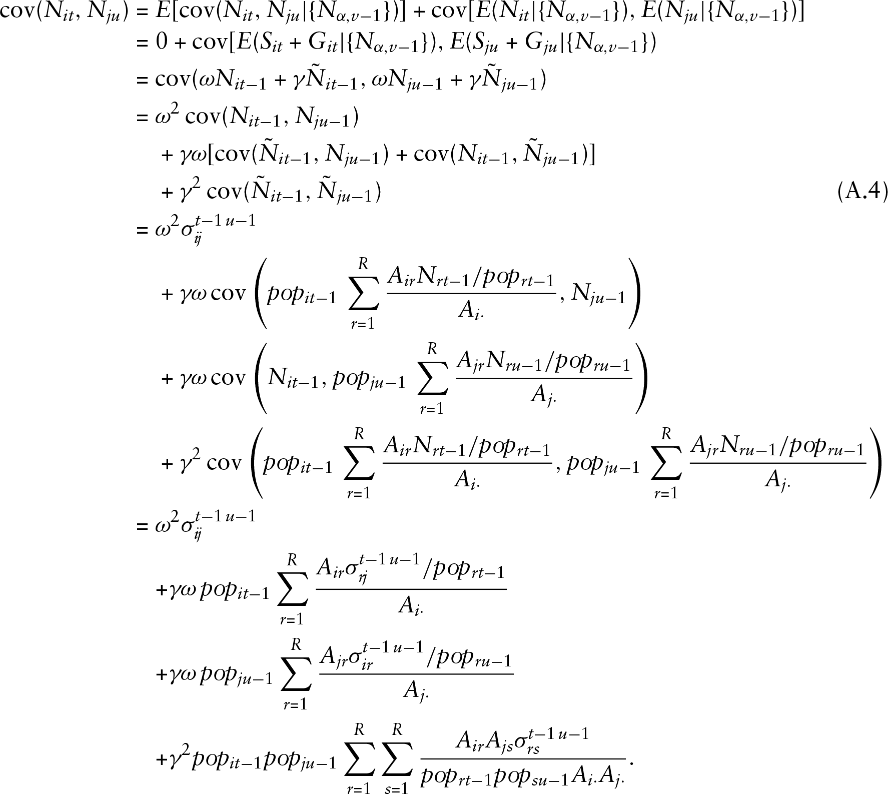
Case 4: Suppose
Average parameter estimates over the
successful simulations for each of the 24 scenarios

There is no covariance term in the third line because cov (Sit,Git|{Nα,v-1})=0.
Table A.1 gives averages of point estimates for parameters
Footnotes
Acknowledgments
The authors disclosed receipt of the following financial support for the research, authorship and/or publication of this article:
Declaration of Conflicting Interests
The authors declared no potential conflicts of interest with respect to the research, authorship and/or publication of this article.
Funding
The authors disclosed receipt of the following financial support for the research, authorship and/or publication of this article:
This investigation was supported by the University of Utah Population Health Research (PHR) Foundation, with funding in part from the National Center for Research Resources and the National Center for Advancing Translational Sciences, National Institutes of Health, through Grant UL1TR002538.