
Abstract
Advancements in computational power and methodologies have enabled research on massive datasets. However, tools for analyzing data with directional or periodic characteristics, such as wind directions and customers’ arrival time in 24-hour clock, remain underdeveloped. While statisticians have proposed circular distributions for such analyses, significant challenges persist in constructing circular statistical models, particularly in the context of Bayesian methods. These challenges stem from limited theoretical development and a lack of historical studies on prior selection for circular distribution parameters.
In this article, we propose a framework for selecting hyperpriors that contracts to a simpler model in circular scenarios, especially when there is insufficient information to guide prior selection. We introduce well-examined Penalized Complexity (PC) priors for the most widely used circular distributions. Comprehensive comparisons with existing hyperpriors in the literature are conducted through simulation studies and a practical case study. Final, we discuss the contributions and implications of our work, providing a foundation for further advancements in constructing Bayesian circular statistical models.
Keywords
Introduction
Advancements in computational power have provided researchers with access to massive and diverse datasets across various fields, enabling the exploration of complex scientific and practical challenges. However, tools for analyzing data with complex structures, such as directional or periodic characteristics, remain underdeveloped and many of these datasets require specialized methods for analysis. For instance, wind directions and bird migration paths are naturally represented on a compass, while hospital patient arrival times and passenger density fluctuations follow a 24 –hour clock (Mardia and Jupp, 2009). The orientation of earthquake epicentres, directions of cosmic rays and stellar objects in astronomy (Cabella and Marinucci, 2009; Ley and Verdebout, 2017; Pewsey and García-Portugués, 2021), joint angles prone to injury, protein structure with angular measures in bioinformatics (Boomsma et al., 2008; Mardia et al., 2018), typhoon trajectories and the analysis of angular components in multivariate extreme value statistics are additional examples of data that align with circular scales. These examples underscore the growing need for statistical frameworks capable of handling circular data.
Directional statistics offers appropriate tools for analyzing such data, with circular distributions—probability distributions defined on the circumference of a circle (Jammalamadaka, 2001) and characterized by angular measures or radians—playing a central role. These methods are crucial for modelling data in fields such as meteorology, earth sciences, bioinformatics, ecology, medicine (Pardo et al., 2016; Vuollo et al., 2016), genetics, neurology, astronomy (Cabella and Marinucci, 2009; Marinucci and Peccati, 2011), image analysis (Jung et al., 2011; Esteves et al., 2018), text mining (Dhillon and Modha, 2001; Banerjee et al., 2005), machine learning (Sra, 2016) and beyond (Ley and Verdebout, 2017; Pewsey and García-Portugués, 2021).
Applying Bayesian methods to circular data, however, poses significant challenges, particularly in the selection of priors—a pivotal step in Bayesian analysis. Unlike Euclidean distributions, circular distributions have unique parameterizations and behaviour, often requiring specialized approaches. For example, in Wallace and Dowe (1993), priors for the concentration parameter κ of von Mises (vM) distribution are constructed through the techniques of Minimum Message Length (MML) (Section 2.1). These priors are also used in Dowe et al. (1996) and Marrelec and Giron (2024). Another popular prior for vM distribution is the joint conjugate prior proposed in Damien and Walker (1999). In addition, in the general procedure for Bayesian analysis with wrapped distributions proposed by Ravindran and Ghosh (2011), the Beta (a,a) prior is employed. Nuñez-Antonio et al. (2011) proposed to fit the Bayesian circular model through the projected normal distribution with normal priors. A prior for the location parameter is often more intuitive to formulate, while priors for the hyperparameters like dispersion parameters are notoriously hard to conceptualize. Moreover, when specific values of the hyperparamaters result in model complexity reduction, care should be taken in the prior construction.
Since circular variables are defined on a compact and curved space rather than in linear Euclidean space, their geometric properties make it difficult to develop strong intuition about their behaviuor. This further complicates prior selection, increasing the risk of using priors that either dominate the posterior or possibly lead to poorly performing models. When a model can be viewed as a complex model containing a simpler counterpart, then a prior allocating insufficient mass to the simpler model can result in inferring a complex model that is not supported by the data. A detailed discussion of the simpler model is presented in Section 3.1.
To address these challenges, we set two goals for this research. First, we establish a prior selection framework for the hyperparameters of a general circular model, inspired by the Penalized Complexity (PC) prior framework proposed by Simpson et al. (2017). The PC prior framework is a reliable choice for constructing default priors, as it balances model complexity and prior informativeness, particularly in scenarios with limited prior knowledge, where objective or uninformative priors are often considered. Second, we derive the explicit expressions for the PC priors for the most commonly used circular distributions’ hyperparameters and provide a way to quantify prior information through a user-defined parameter.
The structure of this article is as follows: Section 2 reviews the most commonly used circular distributions, their properties and existing priors in the literature. Section 3 introduces the proposed framework for prior selection, the procedure for deriving PC priors for circular distributions and the formulations for widely used circular distributions. Section 4 evaluates the proposed priors through comparison studies and simulation studies, while Section 5 demonstrates their application to real-world datasets. Final, Section 6 discusses broader implications and potential directions for future research.
Preliminaries
A proper circular distribution should have a probability density function
Circular distributions in the wrapped family are constructed by taking a distribution defined on ℝ and wrapping it around a circle (modulus by 2π, e.g., wrapped normal distribution, wrapped Cauchy (WC) distribution, wrapped double exponential distribution). The conditioning approach obtains circular distributions through constructing joint distribution of polar coordinates (radius r and angle θ) and finding the conditional distribution
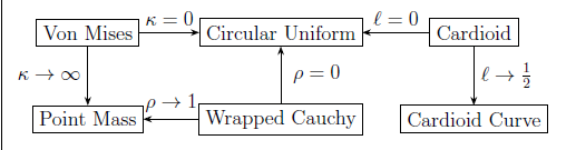
Notably, many of these distributions include the circular uniform distribution as a special case (Figure 1), defined by a probability density function given by
Relationship between popular circular distributions.
and ρ are the concentration parameters for von Mises, cardioid and wrapped Cauchy distributions.
Relationship between popular circular distributions.
and ρ are the concentration parameters for von Mises, cardioid and wrapped Cauchy distributions.
The vM (Mardia and Jupp, 2009), often referred to as the circular normal distribution (Gumbel et al., 1953), is the circular analogue of the normal distribution. It is one of the most widely used and versatile circular distributions (Mardia and Jupp, 2009). Its probability density function is given by:

where μ is the location parameter,
vM density for small (left) and large (right) κ values with μ = π.
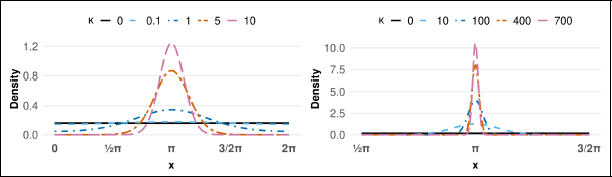
The vM distribution includes the circular uniform distribution as a special case when

Guttorp and Lockhart (1988) proposed a joint conjugate prior for μ and κ, expressed as:

where
Despite its intuitive interpretation, deriving the posterior distribution under this prior requires introducing additional hyperparameters and several latent variables during the sampling process (see Damien and Walker 1999 for details). This construction, however, increases computational complexity and often results in greater Monte Carlo variability of the posterior estimates, owing to the mixing and dependence among latent components. In some cases, particularly when c and R0 are not well chosen or when their combinations convey weak prior information, it may also lead to wider posterior credible intervals.
Dowe et al. (1996) and Marrelec and Giron (2024) both considered two different priors for κ originally proposed by Wallace and Dowe (1993) derived from MML. These priors are defined as:

MML is a Bayesian information-theoretic restatement of Occam's razor, favoring models that describe the data most efficiently. It encodes both the model and the data as one message, where a more complex model requires a longer description and is only preferred if it leads to a shorter overall message. In this sense, priors derived from MML, such as h2 (κ and h3 (κ, naturally penalize overly complex or highly concentrated models unless the data provide strong evidence to support them.
The cardioid distribution is a cardioid perturbation of the circular uniform distribution (Ley and Verdebout, 2017) with probability density function given by

Here,
Cardioid density (left) and wrapped Cauchy density (right) with
for different concentration parameter values.
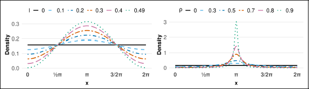
The WC distribution is one of the rare wrapped distribution that has an analytic density function, since its probability density can be expressed in closed form (Ley and Verdebout, 2017). Further details of the WC distribution are discussed in Chapter 3.5.7 of Mardia and Jupp (2009). The probability density function is given by:

The parameter ρ serves as a measure of concentration, with
For Bayesian analysis with a WC distribution, one reasonable choice for the prior for
The circular distributions and priors discussed above show the diversity and utility of existing methods for modelling circular data. However, many of the priors currently in use are either heuristic or tailored to specific cases, lacking a unified framework. This motivates the need for a cohesive approach for default prior selection which can account for the unique properties of circular distributions, as presented in the next section.
This section introduces a framework for constructing contraction hyperpriors for circular distributions that favors simpler circular models. The framework is presented in Section 3.1 together the corresponding prior formulation framework that satisfies them. Specific priors for widely used circular distributions are proposed in Section 3.2.
Penalizing complexity prior for circular models
When there is insufficient information supporting the need for a complicated model, the principle of Occam's razor (MacKay, 2003) suggests favoring simpler alternatives. In this context, model complexity should be carefully considered when specifying prior distributions. One effective way to penalize Bayesian model complexity is through the choice of an appropriate prior, ensuring that it exerts a reasonable influence on the effective complexity of the model. Motivated by this idea, Simpson et al. (2017) proposed the PC prior framework, which is built upon four principles: (1) Occam's razor; (2) measure of complexity; (3) constant rate penalization; and (4) user-defined scaling.
Apart from the first principle, the measure of complexity principle states that the prior should be constructed using a model complexity measure defined by the ‘distance’ d between the model of interest and a simpler base model. The constant rate penalization principle specifies that the PC prior density decays at a constant rate

Finally, the user-defined scaling principle suggests that users should have some understanding of the data, or of the expected model complexity, in order to define the strength of penalization accordingly.
The PC prior framework has been applied in a range of fields. For instance, it has been used in spatial and spatio-temporal modelling (Fuglstad et al., 2019; Cabral et al., 2023; Rodriguez Avellaneda et al., 2025), time-series analysis (Sørbye and Rue, 2017), survival modelling (Van Niekerk et al., 2021) and nonparametric regression (Ventrucci and Rue, 2016). These applications illustrate how PC priors have been used to control model complexity across different modelling contexts, motivating their extension to circular data.
In Euclidean space, statistical measures such as standard deviation and variance are intuitive and straightforward in terms of interpretability. However, as discussed in Section 2, these quantities lose their intuitive meanings for data collected on a circular domain (or transformed into circular form) and concentration parameters are used. The parameterization of the concentration parameter varies among circular distributions but typically includes the value ‘0’ as a special case, representing no concentration (or maximum dispersion). In most common cases, the distribution is simplified to the circular uniform distribution. It should be noted that the mean direction is not likelihood identifiable in the circular uniform distribution.
In contrast, as the concentration parameter increases, most circular distributions tend toward a point mass, representing extreme concentration around a specific direction (mean). An exception is the cardioid distribution which tends toward a cardioid curve rather than collapses into a point mass.
Although most circular distributions exhibit desirable properties when their concentration parameters approach the boundary values, the inference for these distributions can be unstable because the data are defined on a limited range (
This sensitivity and instability indicate the need for an approach to regularizing model complexity. One natural way to achieve this is to view the boundary cases as simpler circular models, which can be regarded as the base model in the PC prior framework, that is, the simplest models representing minimal structure and the most straightforward interpretation. The notion of model complexity can then be described by the measure of complexity principle, where the model complexity is quantified as the distance from the base model. We let

where
Following the formulation of Simpson et al. (2017), the PC prior for a model parameter ξ is defined as an exponential probability density function with respect to the distance, as follows:

where λ is the scaling parameter of the PC prior, defined such that
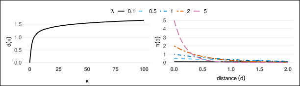
To illustrate how the PC prior behaves with respect to the distance measure, Figure 4 is presented. The left-hand-side plot shows the distance
Distance
between vM distribution and circular uniform distribution (left) and the PC prior density in distance scale for different λ values (right).
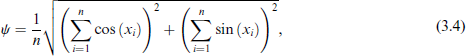
for data
This interpretation is model-independent, as the user can also express ψ explicitly as a function of the model parameter ξ and therefore interpret
This unified approach covers various circular models under one framework. However, it may not be intuitive for users inexperienced with circular data. Therefore, an alternative, more intuitive approach is also suggested.
For most circular distributions, where the bounds of the concentration parameter ξ correspond to the circular uniform distribution and a point mass, a suitable transformation
It is worth noting that the proposed PC priors are flexible in terms of informativeness. That is, they can be either weakly or strongly informative (Simpson et al., 2017), depending on the user's belief about the data. As an illustration, consider selecting the value of λ using the mean resultant length
Von Mises distribution
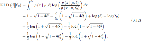
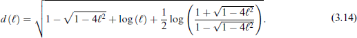
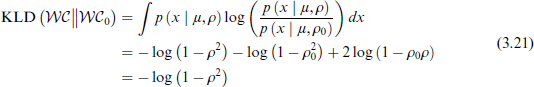
The first step in deriving the PC prior is to compute the KLD. For the vM distribution as defined in Equation 2.1, the KLD is given below:
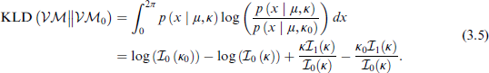
Recall the behaviour of the vM density with respect to changes in the concentration parameter κ (Section 2.1). Two natural choices for base model for the concentration parameter are the circular uniform distribution (
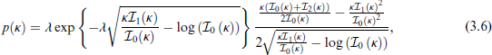
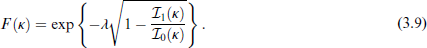
where

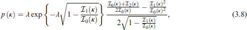
where
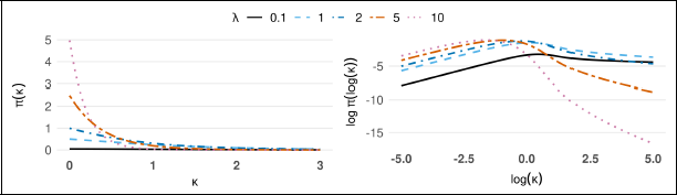
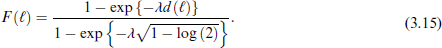
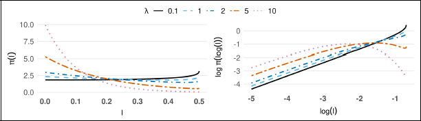
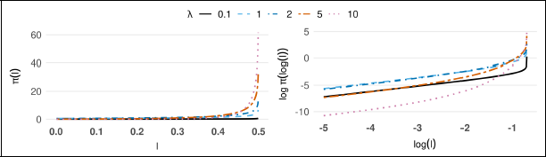
The plots for the density of both PC prior and the corresponding log-log density are presented in Figure 5 (prior with

base model PC prior density (left) and log-log density (right).
base model PC prior density (left) and log-log density (right).
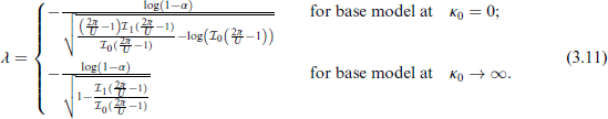
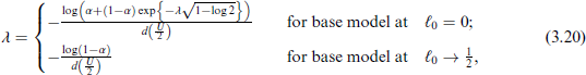
Therefore, the expressions for computing λ for PC priors for κ are given by
For the cardioid distribution as defined in (2.5), we have the KLD as
The base models for the concentration parameter

where
The corresponding CDF is

where

The corresponding CDF is

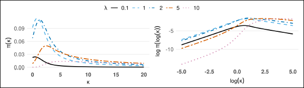
The plots for the density of both PC prior and the respected

base model PC prior density (left) and log-log density (right).
This transformation ensures an intuitive and interpretable way to set U, representing the threshold for the ‘cardiodity rate’ and α, which controls the weight assigned to the tail of the PC prior.
Through calculation, the expressions for computing λ of PC priors of κ are given by
where
Recall that
With this result, the PC prior for ρ is given in Proposition 5.

where

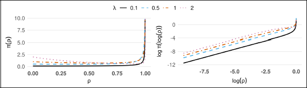
The proof is provided in Appendix A. 3 and the density and
base model PC prior density (left) and log-log density (right).
PC prior (for) density (left) and log-log density (right).
The logic behind our proposed prior selection framework is to assess whether a prior favors simpler models and discourages unnecessarily complex specifications.
The logic behind our proposed prior selection framework is to assess whether a prior favors simpler models and discourages unnecessarily complex specifications. To further illustrate the way of using our framework and to demonstrate the advantages of employing PC priors for circular models, this section compares the proposed priors in Ssubsubsection 3.2.1 with existing priors from the literature. The comparison focuses on their behaviour in both the parameter scale and the distance scale (Subsection 4.1). Additionally, a comprehensive set of simulation studies is presented in Subsection 4.2.
Properties of PC and other common priors
In this section we illustrate the behaviour of the proposed PC prior as well as other priors from the literature for the three cases models under consideration.
Von Mises distribution
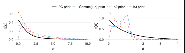
Figure 10 illustrates the behaviour of the PC prior, the popular Gamma(1, b) prior, h2 prior Equation 2.4 and h3 prior Equation 2.4 in both the parameter scale and the distance scale. The distance measure is defined between the vM density and the circular uniform density. For fairness, the scaling parameter λ of the PC prior and the rate parameter b of the Gamma(1, b) prior are calibrated so that both priors share the same median.
Priors for κ in parameter (left) and distance scale (right) with the base model at
. The solid line is the
prior, the dashed line is the Gamma
, the dotted line is the
prior and the dot-dash line is the
prior.
Priors for κ in parameter (left) and distance scale (right) with the base model at
. The solid line is the
prior, the dashed line is the Gamma
, the dotted line is the
prior and the dot-dash line is the
prior.
From the plot of the density on the distance scale, it is evident that the h3 prior assigns zero density at d = 0, indicating that it never suggests the data being uniform. This behaviour implies a preference for more complex models. The Gamma (1, b) prior has reasonable density at the base model, whereas it exhibits a non-monotonic density with a global maximum around
When the base model is at point mass (
Priors for κ in parameter (left) and distance scale with the base model at
(right). The solid line is the
prior, the dashed line is the Gamma
, the dotted line is the
prior and the dot-dash line is the
prior.
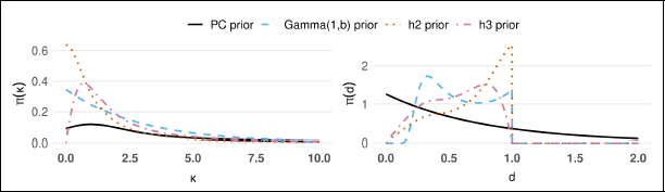
Recall that the h2 and h3 priors are constructed based on the MML criterion, which is intended to penalize model complexity. From the plots given above, we can see that the MML-based priors assign reasonable density to small distances from the base models but do not always allow the model to reach the boundary when the distance measure is defined by Equation 3.2.
Based on these observations, we recommend using the PC prior for the concentration parameter κ of the vM distribution, particularly when limited prior information or belief is available. However, in cases where the data exhibit low concentration, the h2 prior can also be a reasonable alternative.
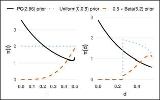
Figures 12 and 13 show the boundary behaviour for the priors for parameter
Priors for
in parameter (left) and distance scale with the base model at
(right). The solid line is the
prior, the dashed line is the Beta
prior and the dotted line is the uniform prior.
Priors for
in parameter (left) and distance scale with the base model at
(right). The solid line is the
prior, the dashed line is the Beta
prior and the dotted line is the uniform prior.
Priors for
in parameter (left) and distance scale with the base model at
(right). The solid line is the
prior, the dashed line is the Beta
prior and the dotted line is the uniform prior.
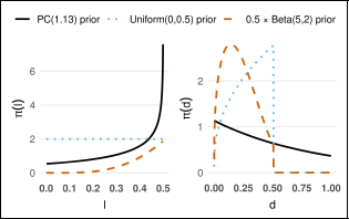
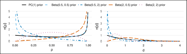
The Beta prior is one of the most commonly used choices for the concentration parameter ρ of the WC distribution. The prior density on both the parameter scale and the distance scale is illustrated in Figure 14. The behaviour of the Beta prior is particularly interesting, as it exhibits different trends near the two boundaries depending on the choice of the a and b hyperparameters. The right-hand-side plot shows that the Beta prior assigns non-zero density at d = 0 only when a < 1, so that it does not exclude the base model a priori. Therefore, a Beta prior with a < 1 can be a suitable prior choice for ρ. When users have sufficient information to set an informative prior, a Beta prior with a < 1 is a reasonable choice, as it maintains the ability to prevent ‘overconfidence’. However, selection of the hyperparameter b significantly influences the behaviour of the Beta prior. Thus, we should always be careful when employing this Beta prior in practice.
Beta prior and PC
prior density in parameter
, left) and distance scale
, right).
Beta prior and PC
prior density in parameter
, left) and distance scale
, right).
In former subsections, we illustrate the way of employing our proposed framework and the behaviour of the discussed priors are illustrated and examined. In this section, we further show the performance of the priors and the robustness of the proposed circular PC priors through comprehensive simulation studies. The simulation study is conducted through comparing the posteriors of the concentration parameter ξ (for vM distribution,
In the study, posterior samples are obtained using the No-U-Turn Sampler, an adaptive variant of Hamiltonian Monte Carlo, implemented through the Stan interface (Carpenter et al., 2017; Stan Development Team, 2025). Sampling is performed using the rstan package version 2.32.7 together with Stan version 2.32.2 to ensure reproducibility. For consistency, the data are sampled from
The convergence behaviour of the model is assessed using the Gelman-Rubin convergence diagnostic,
The simulation study for the priors of the vM distribution is presented below, while the simulation studies for the priors of the cardioid and WC distributions are presented in Appendix B.
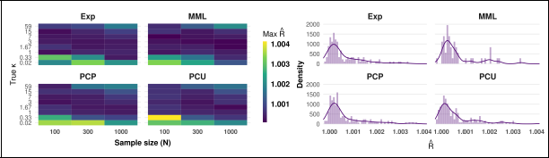
For
values for κ in the simulation study. The left plot shows the maximum
for each setting and the right plot shows the
density by prior. For each setting, the
values for PCU, PCP, and exponential priors are averaged over scaling parameter values, and the
and
priors are averaged and presented under ‘MML’.
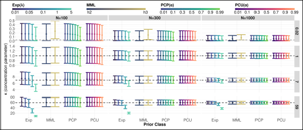
From the results in Figure 16, we can see that both PCU and PCP priors perform consistently across different values of α (resulting in different values of λ), whereas the posterior for Gamma (
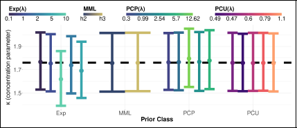
Simulation study for priors on the concentration parameter κ of the vM distribution across different sample sizes and true κ values. The horizontal dashed line indicates the true κ, with points showing posterior means and vertical bars indicating
posterior credible intervals for each prior class.
Through the comparative study presented in this section, we have illustrated a strategy for selecting priors that discourage unnecessarily complex model specifications in circular distributions, emphasizing that the PC prior is consistently an appropriate choice. We acknowledge that other priors may also perform adequately and may outperform the PC prior when sufficient prior information is available to specify them appropriately. The procedure outlined in the previous sections offers a systematic way to examine prior behaviour on the distance scale, allowing practitioners to assess whether a chosen prior may favor model specifications that are more complex than warranted by the available information.
In this section, we present a real-data case study to show the practical performance of the discussed priors. The da used in this study are the wind data (Figure 17) stored in ‘circular’ package (Lund et al., 2017) in R, recorded by a meteorological station in a place named ‘Col de la Roa’ in the Italian Alps. The dataset contains 310 measures of daily wind direction from 29 January 2001 and 31 March 2001, covering the data span from 3 a.m. to 4 a.m. of the day. As a circular analogue of normal distribution, vM distribution is employed for our model and the Bayesian model is the same as expressed in Subsection 4.2. For comparison, the Stan model with
Wind data.
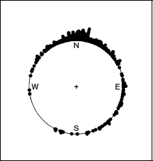
Wind data.
We choose b =0.1, 1, 2, 5 and 10 for the Gamma (1, b) prior. From Figure 17, we can observe that this dataset is not highly concentrated. Therefore, for the PC prior, the circular uniform base model would be a more natural choice compared with the point mass base model. However, for the purpose of comparison and illustration, models with PC prior with both base models are constructed. We choose the scaling parameter λ following the procedure discussed in Section 3.1 with
After fitting the model, the posterior mean and the 95% credible interval for κ are given in Figure 18. In the plot, the horizontal dashed line indicates the frequentist maximum likelihood estimate of κ, with points showing posterior means and vertical bars indicating 95% posterior credible intervals for each prior class. From the plot, the PCU and PCP fit the data well in terms of the stability of credible interval and posterior mean. For this dataset, as a more natural choice, the PCU prior is indeed robust than PCP prior, since the value of scaling parameter λ does not vary much with the same given U and α values.
Posterior means and credible intervals of κ.
We evaluate predictive performance using the expected log predictive density (ELPD), leave-one-out information criterion (LOOIC) (Vehtari et al., 2017), Watanabe-Akaike information criterion (WAIC) (Watanabe and Opper, 2010) and deviance information criterion (DIC) (Spiegelhalter et al., 2002). The ELPD, LOOIC and WAIC are computed through R package loo (Vehtari et al., 2015) version 2.9.0.
The ELPD evaluates out-of-sample predictive accuracy by summing the ELPD for each observation. Under leave-one-out cross-validation (LOO), it is defined as
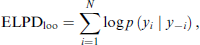
where
In the R package loo,
The LOOIC is defined as LOOIC

We report LOOIC and WAIC together with its standard error and differences relative to the best-performing model and their associated standard errors. The DIC is difined as DIC
The predictive performance metrics are provided in Appendix C. Note that this comparison is intended to further illustrate the stability of the model, ensuring that the estimation does not deteriorate under different prior specifications. Therefore, we do not focus on identifying which prior yields the best predictive fit. For all models evaluated in this case study, all Pareto- k values are
In this application, all models have similar performance with respect to the chosen predictive metrics. The
This practical example demonstrates that the PC priors have stable and comparable performance in circular scenarios, while ensuring that the simpler model is favored a priori.
A framework for selecting priors for parameters of circular distributions is essential for constructing robust Bayesian circular models and for avoiding unnecessarily complex specifications when the parameter space is difficult to interpret. The framework proposed in this article focuses on assessing whether a prior adequately controls model complexity, thereby supporting a more reliable construction of Bayesian circular models. Additionally, it provides a simple and practical way to choose prior hyperparameters so that the resulting priors can be either strongly or weakly informative, depending on the level of prior knowledge available.
The derived PC priors are inherently designed to regularize model complexity and remain stable choices, particularly when prior knowledge is limited or uncertain. In the empirical studies considered in this article, posterior sampling under the PC prior showed no evidence of mixing or numerical instability, including in boundary scenarios. It is worth noting that the advantage of the PC prior lies in its control of model complexity, which helps guard against poorly supported model specifications rather than aiming to achieve the best possible fit. However, when reliable and well-calibrated prior information is available, carefully specified informative priors tailored to a particular setting may provide improved performance. In these situations, the proposed framework can be employed to evaluate prior behaviour with respect to model complexity and assess the suitability of alternative priors. The present analysis does not include a direct numerical diagnostic for excessive model complexity. Instead, model complexity is assessed theoretically by examining whether a prior places sufficient mass near the chosen base model, which can be clearly seen when representing the prior on the distance scale. While a dedicated quantitative metric could further support this assessment, introducing such tools is beyond the scope of this work and may be explored in future research.
Building upon the prior selection strategies and the PC prior for circular distributions addressed in this article, we develop a general Bayesian regression framework capable of handling circular responses, circular covariates, linear covariates or any combination of these (Ye et al., 2026). Future efforts will also focus on extending the prior selection framework to accommodate joint priors and providing conditional PC priors, which are important for handling multi-parameter and multi-modal distributions and models.
Footnotes
Declaration of conflicting interests
The authors declared no potential conflicts of interest with respect to the research, authorship and/or publication of this article.
Funding
The authors received no financial support for the research, authorship and/or publication of this article.
Supplementary materials
References
Supplementary Material
Please find the following supplemental material available below.
For Open Access articles published under a Creative Commons License, all supplemental material carries the same license as the article it is associated with.
For non-Open Access articles published, all supplemental material carries a non-exclusive license, and permission requests for re-use of supplemental material or any part of supplemental material shall be sent directly to the copyright owner as specified in the copyright notice associated with the article.