Application of ARIMA model in classification and prediction of athlete training data

Abstract

Traditional athlete training data classification and prediction models have low accuracy, poor processing of high-dimensional data, and weak dynamic adaptability. Before applying the ARIMA model for classification and prediction, the first step is to use an automated data acquisition system to connect sports devices, collect and clean athlete training data in real time, and securely store and backup it on a central server. The second step is to preprocess the collected data and divide it into training and test sets to ensure the accuracy and generalization ability of the model. The third step is to conduct time-series analysis to identify the time-dependent and seasonal components of athlete training data. The fourth step involves fitting the ARIMA model through differential analysis, stationarity testing, model parameter optimization, residual analysis, rolling forecasting, and ensemble learning, and predicting and classifying athlete training data, so as to improve the accuracy and robustness of the model. The experimental results show that the accuracy of data classification using ARIMA model is the highest, all exceeding 92%, and the average classification accuracy is 2%–16.7% higher than that of other models. Moreover, the prediction errors of the ARIMA model are all below 1.0%. In summary, the application of ARIMA models to classification and prediction of the athlete training data is highly reliable.

Keywords

athlete training data ARIMA model time-series analysis model fitting classification and prediction

Introduction

As sports science and big data technologies develop, the analysis and prediction of athlete training data are becoming increasingly critical. Traditional classification and prediction models are significantly deficient in processing high-dimensional data and in dynamic adaptability, which makes it hard to accurately capture complex patterns and trends in athlete training data. The ARIMA model is an advanced time series analysis method that can effectively handle data with time-dependent and seasonal components, providing more accurate prediction and classification results. Therefore, by applying the ARIMA model to classify and predict athlete training data, not only the accuracy of the model can be improved but also its robustness in practical applications can be enhanced.

The main contributions and innovations of this article are as follows: (1) proposing a method for classification and prediction of athlete training data based on the ARIMA model, which ensures the high quality of data and the reliability of the model through a systematic data acquisition and preprocessing process; (2) combining time-series analysis methods to deeply explore the time-dependent and seasonal components in data; (3) fine-tuning model parameters to ensure the best fitting effect of the model. Finally, through experimental verification, it is demonstrated that the ARIMA model has significant advantages in classification accuracy, prediction error, and high-dimensional data processing, which provides a reliable basis for the analysis and decision-making of athlete training data.

Related work

Classifying and predicting athlete training data is beneficial for comprehensively understanding their performance, progress, and potential problems, revealing potential patterns and trends, so scientific basis can be provided for training and management.^1,2 Classifying and predicting training data is also beneficial for identifying the performance of athletes in high-pressure environments, providing corresponding psychological counseling and intervention measures, and improving their psychological resilience and emotional stability.^3,4 Giles⁵ used athlete tracking data combined with machine learning models for feature extraction and classification. This method effectively detected directional changes during tennis sports, but it had shortcomings such as high data processing complexity and poor model interpretability. Jauhiainen⁶ introduced a novel machine learning method for detecting injury risk factors in young team athletes. By integrating multiple machine learning algorithms, it could accurately identify potential injury risk factors. However, his research had shortcomings in sample size and data diversity. Bunker⁷ proposed a machine learning framework for sports result prediction, which combined multiple machine learning algorithms to improve the accuracy of competition result prediction. However, his research had limitations in terms of applicability to specific sports and the generalization ability of the model. Meng⁸ proposed a dual feature fusion neural network model for sports injury estimation. By integrating multiple features, the prediction accuracy of the model was improved. Although this method performed well in experiments, it faced high requirements for data processing and computational resources in practical applications. In Musa⁹ research, artificial neural networks and k-nearest neighbor classification models were applied to complete the selection task of high-performance archers. By combining the physical fitness and skill parameters of athletes, the accuracy of selection was improved. However, there was still room for improvement in feature selection and model stability in his research. From the above references, it can be seen that different machine learning methods have performed well in improving sports data analysis and prediction, but each still has shortcomings in terms of data processing complexity, model interpretability, universality, and computational resource requirements.

The ARIMA model is different from some complex machine learning models, as it does not require complex assumptions or preprocessing of data.^10,11 Many scholars have utilized the advantages of ARIMA models to predict different data.^12,13 Abonazel¹⁴ study used the ARIMA model to predict Egypt’s Gross Domestic Product (GDP). The data stationarity was ensured through ADF (Augmented Dickey–Fuller) test, and the model order was determined using ACF (autocorrelation function) and PACF (partial autocorrelation function) graphs. The optimal ARIMA model was ultimately selected for prediction. The results indicated that this model had a good prediction effect on Egypt’s GDP and provided high prediction accuracy. Wang¹⁵ proposed a distributed ARIMA model for processing ultra-long time series data. His research adopted a distributed computing framework, dividing ultra-long time series into multiple subsequences. ARIMA models were constructed for local prediction and then the results were merged to obtain global prediction. The results showed that the distributed ARIMA model had high efficiency and scalability in processing large-scale data. Sahai¹⁶ used the ARIMA model to model and predict the COVID-19 epidemic situation in the five most affected countries. In his research, model parameters were estimated using the ordinary least squares method. The results indicated that the ARIMA model could effectively capture the trend of epidemic development and provide short-term predictions. Poongodi¹⁷ applied the ARIMA model to predict Bitcoin prices and conducted time-series analysis on historical Bitcoin price data. The results showed that the ARIMA model had high accuracy in predicting Bitcoin prices. Nath¹⁸ used the ARIMA model to predict wheat yield in India. Firstly, differential processing was performed on the wheat yield data to ensure stationarity, and then the model parameters were determined through ACF and PACF graphs. After estimating and testing the model parameters, the best ARIMA model was ultimately selected for prediction. The results indicated that the ARIMA model performed well in predicting wheat yield and had high prediction accuracy. The ARIMA model is often used to predict heart rate data, detect heart rate abnormalities, and provide early warning of heart attacks or other cardiovascular diseases. The research of the above scholars has shown excellent prediction performance of the ARIMA model. Therefore, this article aims to apply the ARIMA model to classify and predict athlete data.

Application of the ARIMA model

Collection of athlete sports data

The data in this article is sourced from the official database provided by the General Administration of Sport of China. It contains detailed training records of multiple athletes during different training cycles, including key indicators such as training intensity, duration, heart rate, and energy consumption. The specific collection process is shown in Figure 1.

Figure 1.

Collection process of athlete sports data.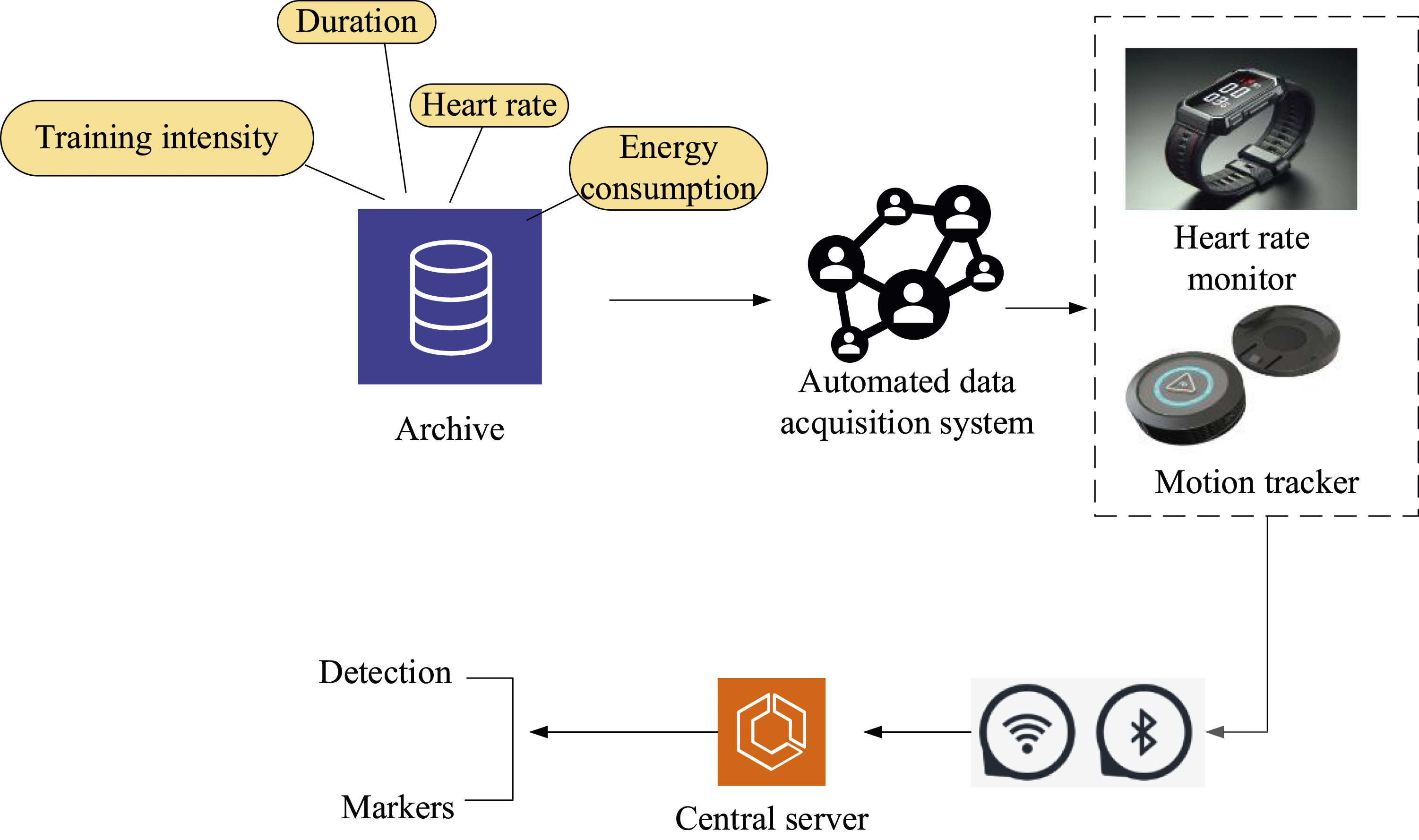

In Figure 1, an automated data acquisition system is used to connect training devices such as heart rate monitors (the model is Polar H10, an electrode heart rate sensor, collecting once per second) and motion trackers to collect real-time training data. These devices are connected to the central server via Bluetooth and Wi-Fi, ensuring real-time data upload and storage. Strict data quality control measures are implemented during the data acquisition process. This includes real-time monitoring of data flow, automatic detection, and labeling of abnormal data points. Heart rate values or unreasonable exercise intensity records that exceed the normal range are manually reviewed, and whether to retain or remove them is decided based on the review results. By implementing measures such as data encryption, access control, data anonymization and de-identification, regulatory compliance, and security training and awareness, the privacy and security of collected data are effectively safeguarded.

Data from different devices and time periods is integrated, and data cleaning techniques are used to remove duplicate records, correct formatting errors, and unify data units to ensure data consistency and availability. All collected data is stored in a secure server, using distributed storage technology to improve data access speed and reliability. At the same time, regular data backup strategies are implemented to ensure the security and integrity of data.

Data preprocessing

Missing values are a common issue in athlete training data, and improper handling can seriously affect the performance of the model.^19,20 Therefore, a preliminary analysis of the data is conducted to identify the location and quantity of missing values using descriptive statistical methods. For continuous data, use mean imputation method to handle missing values:

X_{f i l l} = \frac{1}{N} \sum_{i = 1}^{N} X_{i}

(1)

The variable definition of the formula for processing missing values is shown in Table 1.

Table 1.

Variable interpretation of the formula for processing missing values.

Sequence	Variable	Meaning
1	$X_{f i l l}$	The value after imputation
2	$N$	The number of non-missing data points
3	$X_{i}$	The non-missing observations

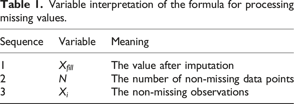
For categorical data, the mode imputation method is used, which replaces missing values with the most frequently occurring category. This method can maintain the distribution characteristics of categorical variables and avoid bias caused by missing values.

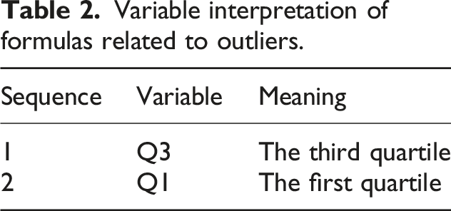
Outlier types include data input errors, device faults, and abnormal motion events. The presence of outliers can have a negative impact (increased sensitivity and reduced generalization) on the training and prediction results of the model, so box-plots and interquartile range (IQR) methods are used to identify outliers. The first quartile and third quartile are calculated, and then the IQR^21,22 is calculated to determine the upper and lower bounds of outliers: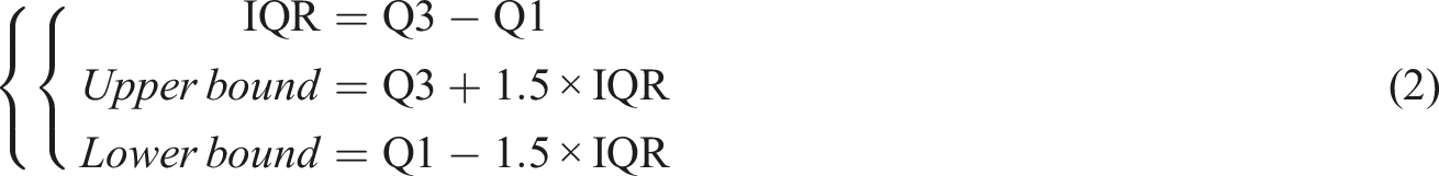

{{\begin{cases} IQR = Q 3 - Q 1 \\ U p p e r b o u n d = Q 3 + 1.5 \times IQR \\ L o w e r b o u n d = Q 1 - 1.5 \times IQR \end{cases}

(2)

The variable definition of formula (2) is shown in Table 2.

Table 2.

Variable interpretation of formulas related to outliers.

Sequence	Variable	Meaning
1	$Q 3$	The third quartile
2	$Q 1$	The first quartile

Values that exceed the upper and lower bounds are considered as outliers and are replaced with the corresponding bound values. In order to handle scale differences in data, Z-score normalization is applied to all numerical features, so that different features have the same measurement scale.

For features that exhibit nonlinear relationships with output variables, logarithmic transformation is performed to improve their distribution characteristics. The formula is as follows:

Y^{‘} = \log (Y + 1)

(3)

Among them, $Y^{‘}$ is the transformed value and $Y$ is the raw data value. Adding 1 here is to avoid taking the logarithm of 0. The skewed distribution of the data is reduced, making it closer to a normal distribution, and thus improving the fitting effect of the model.

The moving average method is used to adjust for seasonal fluctuations in athlete training data^23,24:

S_{t} = \frac{1}{m} \sum_{j = - k}^{k} X_{t + j}

(4)

Among them, $S_{t}$ is the adjusted value at time point $t$ ; $X_{t + j}$ is the value of time point $t + j$ in the original sequence; $\frac{1}{m} Σ_{j = - k}^{k}$ is the moving average window size.

The moving average is subtracted from the raw data to obtain adjusted seasonal data, thereby removing seasonal components. The adjusted seasonal data better reflects the trend and changes in training effectiveness.

Finally, the dataset is divided into training and test sets in chronological order. The impact of different data segmentation strategies on model performance is significant. Random segmentation is suitable for non-time series data, but it may lead to time series data leakage. Time series segmentation is suitable for time series data, which can preserve temporal dependencies and avoid data leakage. The training set is used for model training, and K-fold cross-validation is used during the training process. The test set is used to validate the prediction performance of the model. To ensure the generalization ability of the model, it is necessary to ensure the continuity of the training and test sets in time, and to avoid data leakage.

Time-series analysis

The goal of time-series analysis is to identify the time-dependent and seasonal components of data, laying the foundation for the application of ARIMA models. Compared with traditional moving average method, exponential smoothing method, and modern STL (Seasonal and Trend decomposition using Loess), it can be found that STL has significant advantages in processing athlete training data. It can accurately capture long-term trends and seasonal variations in data, as well as effectively handle outliers and noisy data. Athlete training data is visualized using time series data graphs, observing the trends, seasonality, and periodicity of the data. The data from January 1, 2022 to January 1, 2023 is taken as an example, as shown in Figure 2. In Figure 2, the moving average is calculated and plotted to smooth time series data and further identify long-term trends and periodic fluctuations. The window size of the moving average is 7 days.

Figure 2.

Time series data graph.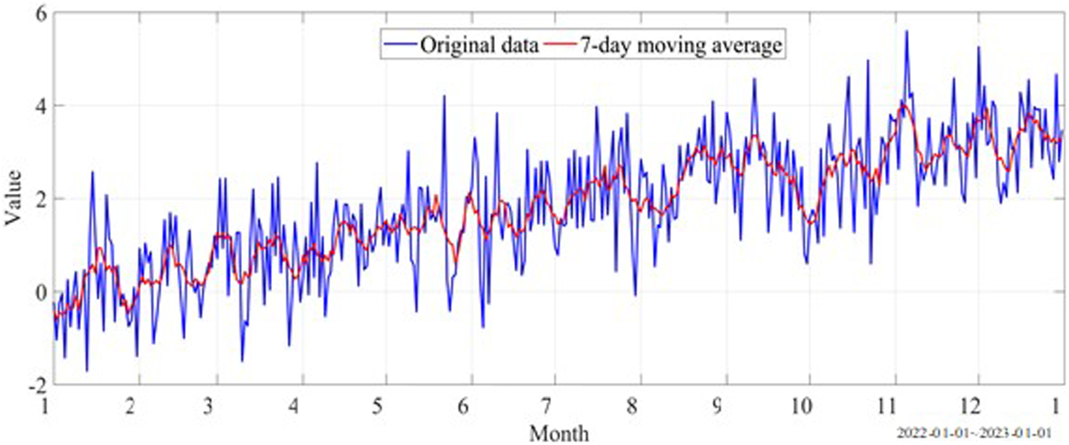

The ADF statistic and corresponding p-value are calculated using the ADF test to determine whether the sequence is stationary.^25,26 The formula is as follows:

{Δ Y}_{t} = α + β t + γ Y_{t - 1} + \sum_{i = 1}^{k} δ_{i} Δ Y_{t - i} + ϵ_{t}

(5)

α

represents a constant term;

β t

represents the time trend term;

γ Y_{t - 1}

represents the autoregressive term;

\sum_{i = 1}^{k} δ_{i} Δ Y_{t - i}

represents the lag term;

k

is the lag order;

ϵ_{t}

represents the error term.

If the p-value is less than the significance level (0.05) and the null hypothesis is rejected, the sequence is stationary. KPSS (Kwiatkowski–Phillips–Schmidt–Shin) test is used: calculating KPSS statistics and corresponding critical values to determine whether the sequence is stationary. If the KPSS statistic is greater than the critical value and the null hypothesis is rejected, then the sequence is non-stationary.

If the sequence is unstable, differential transformation is used for stationarization. By calculating first-order and second-order differences to eliminate trend and seasonal components in the data, the sequence satisfies the assumption of stationarity.

After analyzing the stationarity of the sequence, ACF and PACF are used to analyze the autocorrelation characteristics of the sequence. ACF is used to display the correlation between the sequence and its lag value, and to identify the MA (moving average) component in the sequence^27,28: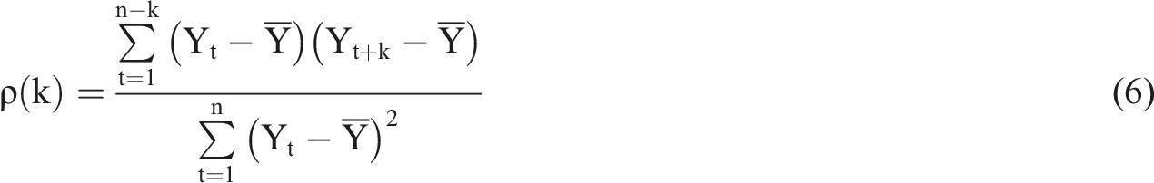

ρ (k) = \frac{\sum_{t = 1}^{n - k} (Y_{t} - \bar{Y}) (Y_{t + k} - \bar{Y})}{\sum_{t = 1}^{n} {(Y_{t} - \bar{Y})}^{2}}

(6)

\bar{Y}

refers to the sample mean.

PACF is used to display the partial correlation between a sequence and its lag value, and to identify the AR (autoregressive) components in the sequence. Based on the significant peaks in the ACF and PACF graphs, the order of the ARIMA model, that is, the values of AR (p) and MA (q), is preliminarily determined. When the ACF graph gradually decays after a certain lag order, and the PACF graph is truncated at that lag order, the AR model is selected; on the contrary, the MA model is selected.

For seasonal time series, seasonal difference method is applied to eliminate seasonal components. Time series with structural mutations should be detected using CUSUM (cumulative sum) and Pettitt tests. First, the cumulative sum statistic is calculated and a CUSUM graph is drawn to determine whether there are significant mutation points in the sequence. Then, the Pettitt statistic and its corresponding significance level are calculated to detect mutation points in the sequence. If the p-value is less than the significance level (0.05), there is a mutation point in the sequence. For complex time series, STL (Seasonal and Trend decomposition using Loess) is applied to decompose the sequence into trend, seasonality, and residual components by specifying the window size. The decomposed components are observed, and trend changes and periodic fluctuations in the data are identified. In contrast, ARIMA models have stronger predictive ability and higher flexibility, and they can be adapted to various time series data through parameter adjustment, especially performing well in predicting future data.

Model fitting and prediction classification

When applying the ARIMA model to classify and predict athlete training data, selecting appropriate model parameters (p, d, and q) is crucial. p controls the use of the number of past observations to predict the current value. High p-values increase model complexity and may lead to overfitting. d controls the number of data differentials to make the sequence stationary. Appropriate d-values can eliminate trends, but excessively high d-values may lead to excessive noise. q controls the use of past prediction errors to predict the current value. High q-values increase model complexity and may lead to overfitting.

The first-order differencing is performed on the raw data, and the ADF test is used to perform stationarity test on the difference data. If the data is still non-stationary, second-order differencing is continued to be used. Non-stationary data can undergo logarithmic transformation to reduce its volatility and make it closer to a stationary state. When the differentiated data meets the stationarity requirements, the number of differences (d) is recorded. The values of (p) and (q) are determined by observing significant lag orders through ACF and PACF graphs.

ACF and PACF graphs are used to determine the initial order of the model. AIC (Akaike Information Criterion) and BIC (Bayesian Information Criterion) are used to further optimize the order selection, ensuring a balance between the complexity and accuracy of the model.

The maximum likelihood estimation (MLE) method is used to set initial parameter values and calculate the initial logarithmic likelihood function value. The numerical optimization algorithms are used to gradually adjust parameter values to maximize the logarithmic likelihood function.^29,30 Optimizing and converging to the optimal estimate of parameters are continued iteratively, completing parameter estimation. The formula is as follows:

L (θ | Y) = - \frac{n}{2} \ln (2 π σ^{2}) - \frac{1}{2 σ^{2}} \sum_{t = 1}^{n} {(Y_{t} - μ_{t})}^{2}

(7)

σ^{2}

refers to the data variance and

μ_{t}

refers to the

t

-th data point in the predicted value sequence of the model.

The estimated parameters are substituted into the ARIMA model, and the least squares method is used for model fitting. PCA (Principal Component Analysis) is used to reduce the dimensionality of high-dimensional training data, extract main features, and reduce computational complexity, while maintaining the main information of the data.

The fitting effect of the model is tested through residual analysis. The histogram is used to determine whether the residual satisfies the normal distribution. For residuals that do not meet the normal distribution, data transformation, model adjustment, outlier processing, and non-parametric methods are used to improve the normality of residuals and improve the prediction effect of the model. A residual sequence diagram is drawn and if the residual is white noise (mean is zero, and variance is constant, without autocorrelation) is checked. Ljung–Box test is used to perform autocorrelation test on residuals, ensuring that there is no significant autocorrelation in the residual sequence. Based on residual analysis and model validation results, the model parameters are adjusted for iterative optimization until the model reaches the best fitting effect.

After completing the fitting of the ARIMA model, athlete training data is predicted and classified. Fitted ARIMA models are used for short-term and long-term prediction of training data. At each prediction step, the model is updated with the previous predicted values, which is rolling forecasting. During the prediction process, the predicted and actual values of each step are recorded for subsequent analysis of prediction errors. Inverse differential transformation is applied to restore the predicted results to the original scale, ensuring that the predicted results are consistent with the actual data. The selection of prediction error indicators includes mean-square error, root mean squared error, and mean absolute error.

Statistical features of time series (mean, variance, and autocorrelation coefficient) are extracted, and training data is converted into feature vectors suitable for classification. Grid search and cross-validation techniques are used to find the optimal combination of model parameters. Comparing the performance of the model with default parameters and optimized parameters, the accuracy of the model with default parameters is 70%. The model performance with optimized parameters has an accuracy rate of 85%. It is evident that the performance of the model improves after using grid search and cross-validation techniques. The extracted feature vectors are input into the model for classification tasks. Combining prediction and classification results, the features of categories with high classification errors are analyzed, and feature engineering and model parameter adjustment are performed. Finally, ensemble learning techniques (stacking and voting) are used to integrate the prediction results of multiple classification models, improving the accuracy and robustness of classification. The training data characteristics of different sports events may vary. The ARIMA model has good applicability in handling training data with regular periodicity and gradual improvement, but its limitations are more obvious for sports projects affected by multiple external factors and high-dimensional data.

Improving overall model performance also requires ensemble learning. In this article, Bagging (Bootstrap Aggregating) is selected to extract multiple subsets from the raw dataset with replacement. Then a base learner is trained for each subset (set to 100). Finally, the prediction results of these base learners are combined through voting or averaging.

Evaluation of performance tests

Classification accuracy

To verify the effectiveness of using ARIMA model (M1) for classifying and predicting athlete training data, random forest model (M2), support vector machine model (M3), convolutional neural network model (M4), and long short-term memory model (M5) are selected for comparison. Random forests can handle high-dimensional data and have good robustness to outliers and noise. Support vector machines have demonstrated strong classification capabilities in handling small sample, nonlinear, and high-dimensional pattern recognition and can flexibly handle nonlinear problems through different kernel functions. Convolutional neural networks effectively extract local features from time series data through one-dimensional convolution. As a deep learning model, they can automatically learn complex data representations and are suitable for high-dimensional time series data. Long short-term memory models are adept at processing sequential data, capturing long-term dependencies in time series, and effectively avoiding gradient vanishing problems through their unique memory unit structure, making them suitable for long-term sequence prediction. By comparing these models, the performance of different types of models in athlete training data classification and prediction tasks can be comprehensively evaluated.

As the sample size increases, the performance of the model gradually improves. Training data is randomly selected from 250 athletes, with 10 features including heart rate, step count, speed, training time, calorie consumption, blood oxygen level, sleep time, body fat rate, heart rate variability, and sports type. The time span is 1 year, and the data is recorded once a day. The dataset is divided into training sets (70%) and test sets (30%) to ensure the temporal continuity of the training and testing data.

According to the training performance of athletes, the data is manually labeled into three categories: efficient training (L1), moderate training (L2), and inefficient training (L3). The imputation of missing values, processing of outliers, standardization, and adjustment of seasonal data are performed on training data (section 3.2, data preprocessing, shows details). To ensure fairness in comparison, all models use the same preprocessed data, and each model is trained using the training set. Each model undergoes 10 rounds of cross-validation to avoid overfitting and evaluation bias.

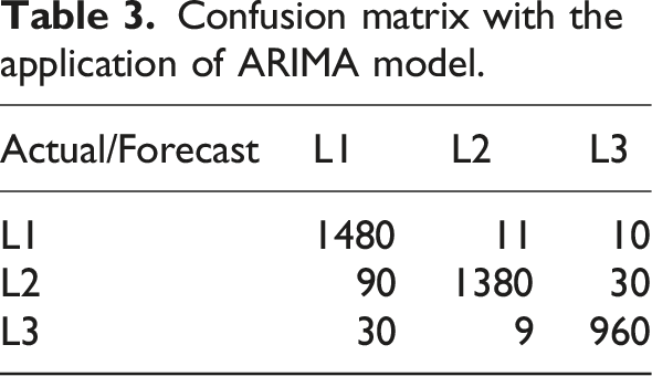
The confusion matrix is used to calculate the classification accuracy of each model on the test set. The test set contains 4000 data points, including 1600 for efficient training, 1400 for moderate training, and 1000 for inefficient training. The comprehensive application of data preprocessing and partitioning, parallelization and distributed computing, model simplification and optimization, incremental training, and online learning to optimize the training time of ARIMA models on large data sets can effectively improve the computational efficiency. The confusion matrices of each model are shown in Tables 3–7.

Table 3.

Confusion matrix with the application of ARIMA model.

Actual/Forecast	L1	L2	L3
L1	1480	11	10
L2	90	1380	30
L3	30	9	960

Table 4.

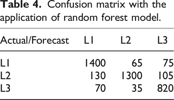
Confusion matrix with the application of random forest model.

Actual/Forecast	L1	L2	L3
L1	1400	65	75
L2	130	1300	105
L3	70	35	820

Table 5.

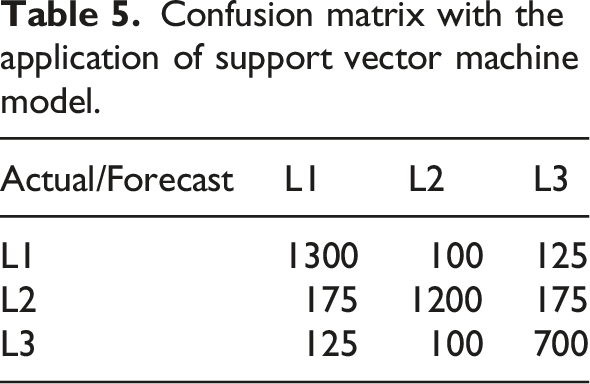
Confusion matrix with the application of support vector machine model.

Actual/Forecast	L1	L2	L3
L1	1300	100	125
L2	175	1200	175
L3	125	100	700

Table 6.

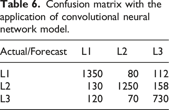
Confusion matrix with the application of convolutional neural network model.

Actual/Forecast	L1	L2	L3
L1	1350	80	112
L2	130	1250	158
L3	120	70	730

Table 7.

Confusion matrix with the application of long short-term memory model.

Actual/Forecast	L1	L2	L3
L1	1450	23	20
L2	100	1350	40
L3	50	27	940

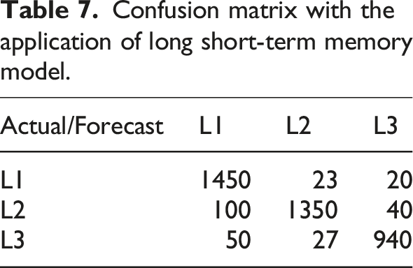
Table 3 shows that among the 4000 data points included in the test set, out of 1600 data points of L1, 1480 are correctly classified; 90 are misclassified as L2; 30 are misclassified as L3. Out of 1400 data points in L2, 1380 are correctly classified; 11 are misclassified as L1; 9 are misclassified as L3. Out of the 1000 data points in L3, 960 are correctly classified; 10 are misclassified as L1; 30 are misclassified as L2.

Table 4 shows that out of 1600 data points in L1, 1400 are correctly classified; out of 1400 data points in L2, 1300 are correctly classified; out of the 1000 data points in L3, 820 are correctly classified.

Table 5 shows that out of 1600 data points in L1, 1300 are correctly classified; out of 1400 data points in L2, 1200 are correctly classified; out of 1000 data points in L3, 700 are correctly classified. Specifically, the accuracy of the support vector machine model in classifying and predicting athlete training performance is lower than that of the random forest model and ARIMA model, and it has significant errors in distinguishing between efficient training, moderate training, and inefficient training.

Table 6 shows that out of 1600 data points in L1, 1350 are correctly classified; out of 1400 data points in L2, 1250 are correctly classified; out of 1000 data points in L3, 730 are correctly classified. The misclassified data points in L1 and L3 are both above 100.

In Table 7, out of 1600 data points in L1, 1450 are correctly classified; out of 1400 data points in L2, 1350 are correctly classified; out of the 1000 data points in L3, 940 are correctly classified. These data indicate that the long short-term memory model has high accuracy in classifying and predicting athlete training data, significantly outperforming random forest, support vector machine, and convolutional neural network models.

The classification accuracy of different models is calculated based on the data from Tables 3–7, as shown in Figure 3.

Figure 3.

Classification accuracy of different models.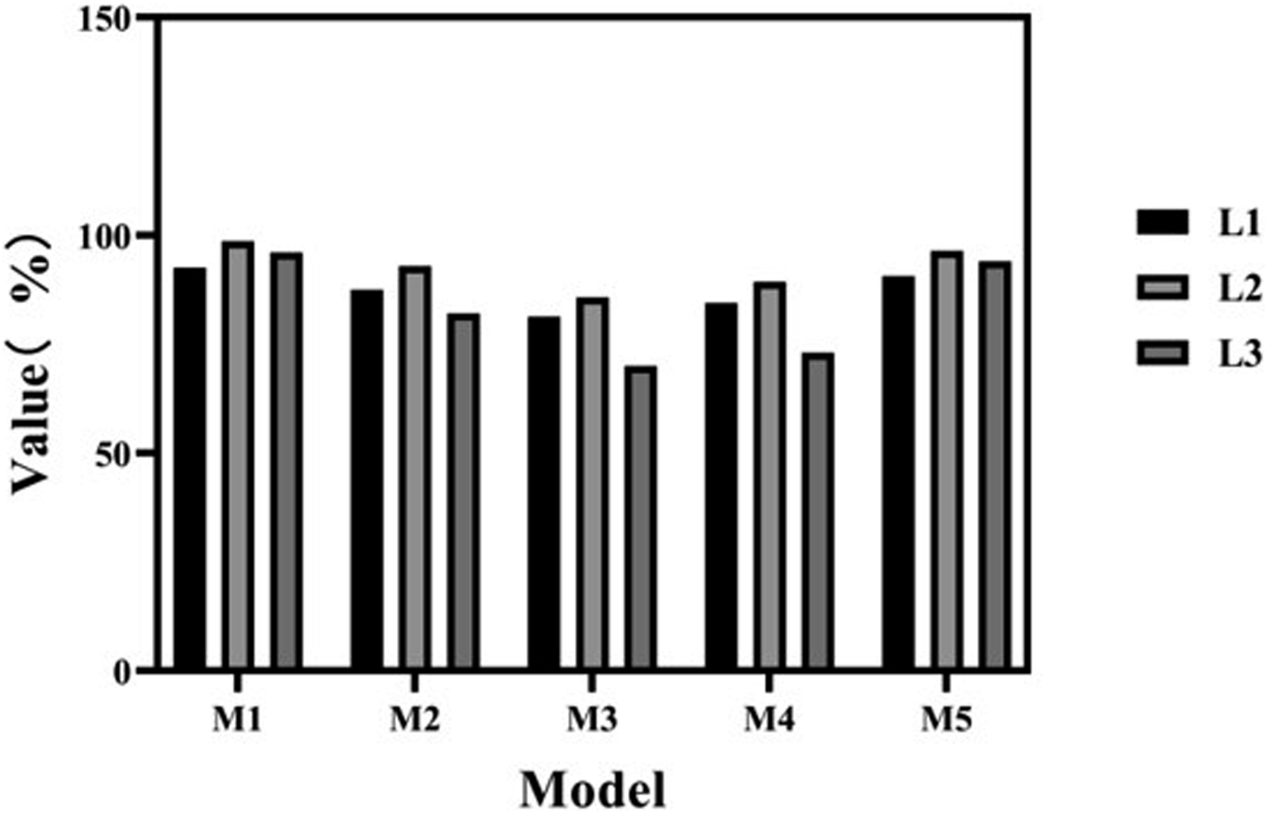

In Figure 3, M1 has the highest accuracy in data classification, all exceeding 92%, followed by M5 with an accuracy of over 90%. The accuracy of data classification in M3 is the lowest.

The average classification accuracy is calculated based on the data in Figure 3, as shown in Figure 4.

Figure 4.

Average classification accuracy of different models.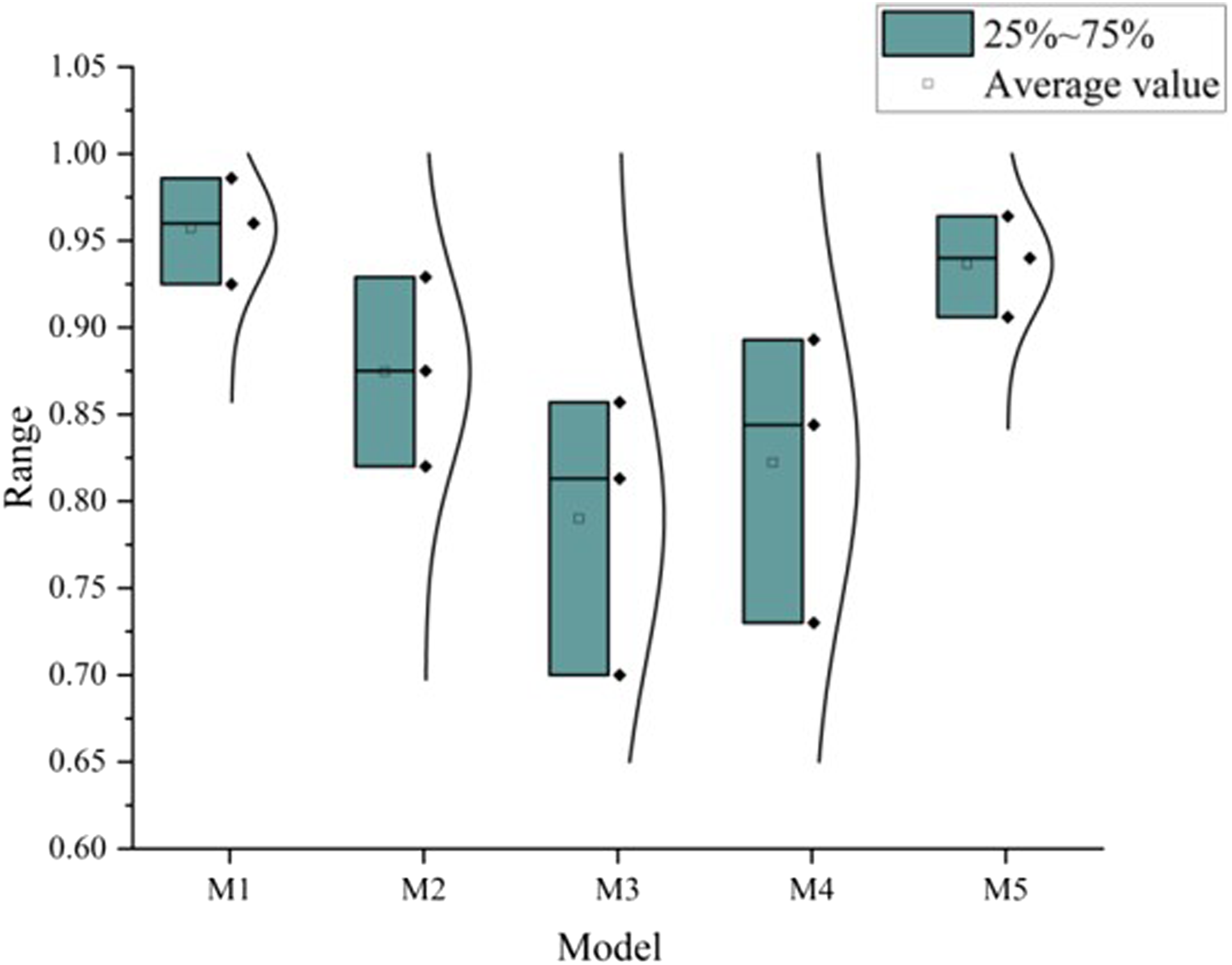

In Figure 4, the average classification accuracy of M1 is the highest at 95.7%, followed by M5, with an average classification accuracy of 93.7%. The average classification accuracy of M3 is the lowest, with 79%. The data shows that the application of ARIMA model ensures the classification of athlete training data. Compared to other models, its classification accuracy is 2%–16.7% higher.

Athlete training data is real-time. To ensure the effectiveness of the experiment, the dataset is expanded by selecting athlete data from different sports events (football, basketball, athletics, swimming, and gymnastics), with 500 athletes selected for each sports event to ensure the representativeness of the data sample. As with the above operation, it can be calculated that the average classification accuracy of M1 is still the highest, at 93.68%. Then they are sorted by high and low, M5, M2, M4, and M3 in sequence, with 91.93%, 90.53%, 88.97%, and 85.23%, respectively.

Prediction accuracy

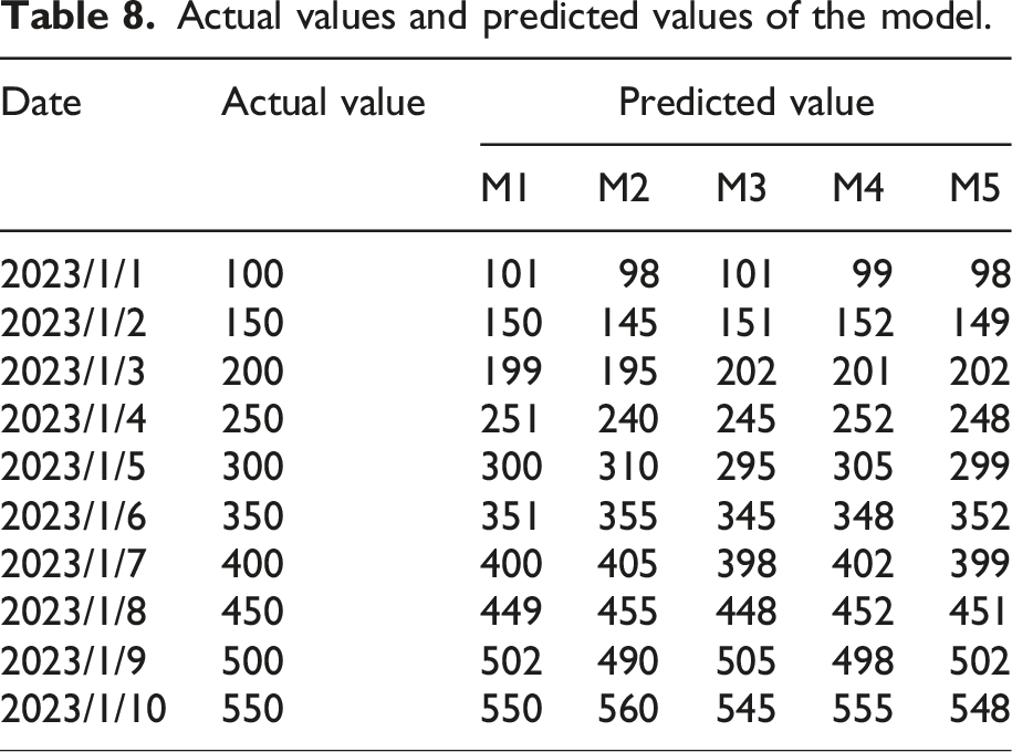
Using the training data of actual athletes for case analysis can better demonstrate the specific application effect of the ARIMA model in classification and prediction. The actual training data and corresponding model prediction data of 10 days of athlete sports are selected, and the results are shown in Table 8. Table 8 provides a detailed list of the actual data values from January 1 to January 10, 2023, as well as the corresponding predicted values for each model. If the difference between the predicted value and the actual value does not exceed 1.5%, the prediction is considered accurate.

Table 8.

Actual values and predicted values of the model.

Date	Actual value	Predicted value
Date	Actual value	M1	M2	M3	M4	M5
2023/1/1	100	101	98	101	99	98
2023/1/2	150	150	145	151	152	149
2023/1/3	200	199	195	202	201	202
2023/1/4	250	251	240	245	252	248
2023/1/5	300	300	310	295	305	299
2023/1/6	350	351	355	345	348	352
2023/1/7	400	400	405	398	402	399
2023/1/8	450	449	455	448	452	451
2023/1/9	500	502	490	505	498	502
2023/1/10	550	550	560	545	555	548

The prediction error is calculated based on the data in Table 8, and the results are shown in Table 9.

Table 9.

Prediction errors of each model.

Date	M1	M2	M3	M4	M5
2023/1/1	1.0%	2.0%	1.0%	1.0%	2.0%
2023/1/2	0	3.3%	0.7%	1.3%	0.7%
2023/1/3	0.5%	2.5%	1.0%	0.5%	1.0%
2023/1/4	0.4%	4.0%	2.0%	0.8%	0.8%
2023/1/5	0	3.3%	1.7%	1.7%	0.3%
2023/1/6	0.3%	1.4%	1.4%	0.6%	0.6%
2023/1/7	0	1.3%	0.5%	0.5%	0.3%
2023/1/8	0.2%	1.1%	0.4%	0.4%	0.2%
2023/1/9	0.4%	2.0%	1.0%	0.4%	0.4%
2023/1/10	0	1.8%	0.9%	0.9%	0.4%

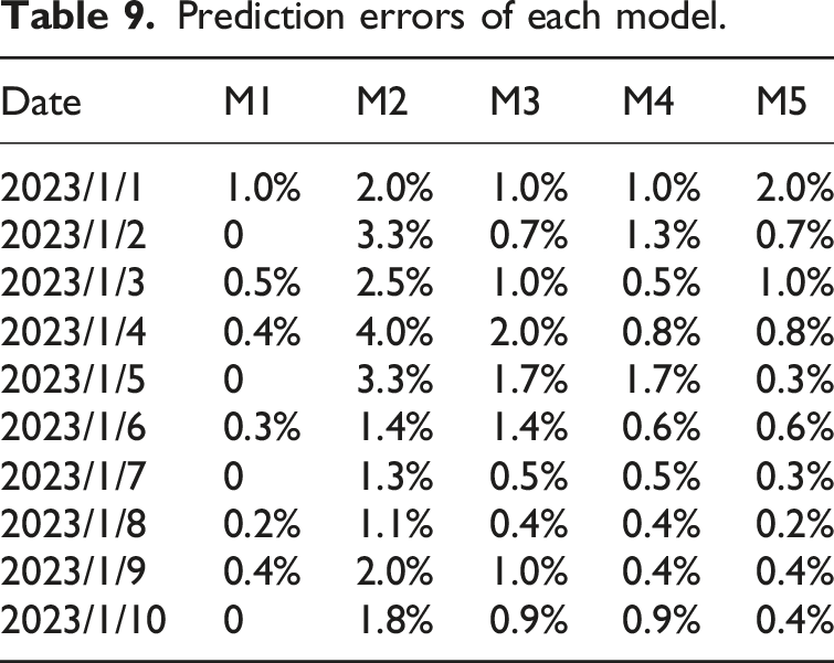
Table 9 provides a detailed calculation of the prediction errors for each model within 10 days. The prediction error of M1 on all dates is below 1.0%. In contrast, M2 has a larger prediction error, exceeding 1.5% on many dates. The prediction error of M3 is relatively stable, with only 2 days of error exceeding 1.5%. The prediction error of M4 and M5 is mostly within 1.5%. Through comparative analysis, it can be seen that M1 has the smallest prediction error and more accurate prediction results, and it can better reflect the actual training data.

The average prediction error of each model is calculated based on the data in Table 9, as shown in Figure 5.

Figure 5.

Average prediction error of each model.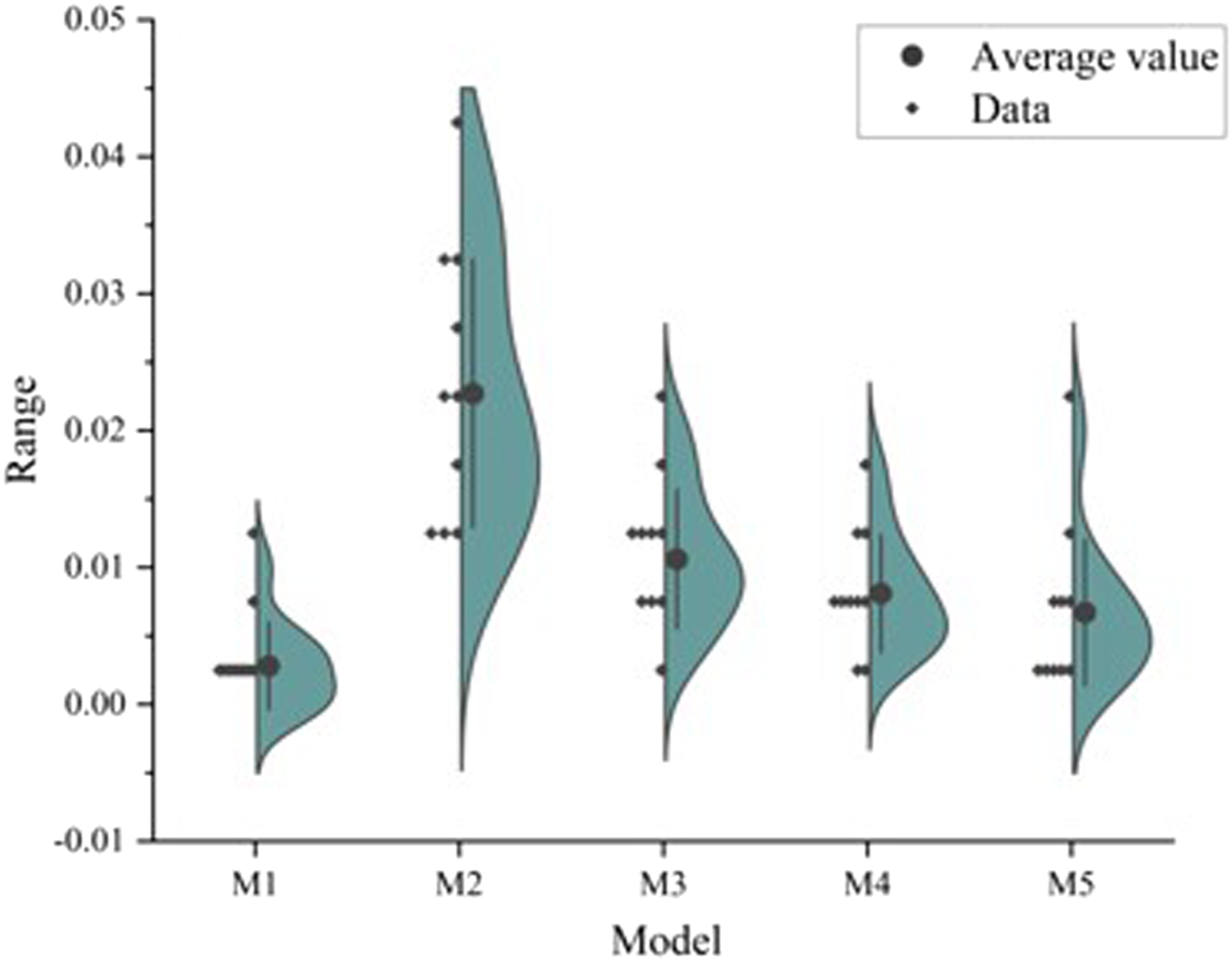

In Figure 5, the mean prediction error of M2 is the highest, indicating a high degree of instability in the model’s predictions. The average prediction error of M1 is significantly lower than other models. The number of accurately predicted days from the data in Table 9 is divided by the total number of days to obtain the prediction accuracy. The details are shown in Table 10.

Table 10.

Prediction accuracy of each model.

	M1	M2	M3	M4	M5
Total days	10	10	10	10	10
Accurately predicted days	10	3	8	9	9
Prediction accuracy	100%	30%	80%	90%	90%

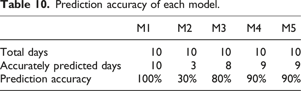
Table 10 clearly shows that M1 has the highest prediction accuracy, reaching 100%, followed by M4 and M5, both at 90%, while M3 has an accuracy of 80%, showing relatively good performance. M2 has the lowest prediction accuracy, only 30%. These results indicate that M1 is the most reliable prediction model, followed by M4 and M5, while M2 has lower prediction accuracy and needs further improvement.

In addition to evaluating the accuracy and prediction error of the ARIMA model, the stability of the model on different time windows and datasets is good and does not require improvement.

High-dimensional data processing

PCA is used to reduce the dimensionality of high-dimensional data, retaining 95% of the data variance. Five models, M1, M2, M3, M4, and M5, are trained using the dimensionality reduced data. Then the trained models are used to fit and predict high-dimensional data. The training and prediction time of each model when processing high-dimensional data is recorded. Simultaneously the memory usage of each model when processing high-dimensional data is monitored, as shown in Table 11.

Table 11.

High-dimensional data processing situations.

Model	Training time (s)	Prediction time (s)	Memory usage (MB)
M1	90	1.5	45
M2	150	4	130
M3	180	8	180
M4	250	15	250
M5	320	20	300

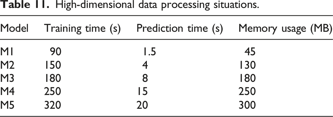
In Table 11, M1 has the shortest training time of only 90 seconds, which is significantly better than other models, indicating its high efficiency in high-dimensional data processing. The training time of M2 and M3 is relatively short, with 150 seconds and 180 seconds, respectively. The training time of M4 and M5 is relatively long, with 250 seconds and 320 seconds, respectively.

M1 has the shortest prediction time, only 1.5 seconds, demonstrating its fast prediction ability. The prediction time of M2 and M3 is 4 seconds and 8 seconds, respectively, showing good performance. The prediction time of M4 and M5 is relatively long, with 15 seconds and 20 seconds, respectively.

M1 has the least memory usage, only 45 MB, which is a significant advantage in resource-limited environments. The memory usage of M2 and M3 is 130 MB and 180 MB, respectively. M4 and M5 use more memory, with 250 MB and 300 MB, respectively.

From the above results, it can be seen that M1 has significant advantages in processing high-dimensional data. It not only has shorter training and prediction time but also has the least memory usage, making it suitable for classifying and predicting training data in environments with limited computational resources. Although other models perform well in certain aspects, overall, M1 is more efficient and resource friendly.

Conclusion

This article uses the ARIMA model-based athlete training data classification and prediction method to collect and preprocess athlete training data, and uses time-series analysis to identify the time-dependent and seasonal components of the data. Finally, the best parameter fitting model is selected for classification and prediction. Experiments have shown that the ARIMA model significantly outperforms other models in classification accuracy, with small prediction errors and strong high-dimensional data processing capabilities. However, the ability of this article to handle extreme outliers and nonlinear trends is limited. The ARIMA model performs well in classifying and predicting athlete training data, helping coaches and athletes understand training effectiveness and optimize training plans, thereby preventing overtraining and injuries, improving performance and recovery efficiency. Future research directions include deep learning feature extraction to enhance model predictive ability, multi-source data fusion to provide comprehensive support, and the application of more nonlinear and hybrid models to better capture complex data patterns and trends. Optimizing model parameters and improving data collection systems can further enhance the accuracy and practicality of the model.

Statements and declarations

Footnotes

Conflicting interests

The author(s) declared no potential conflicts of interest with respect to the research, authorship, and/or publication of this article.

Funding

The author(s) disclosed receipt of the following financial support for the research, authorship, and/or publication of this article: This work was supported by the Hunan Provincial Department of Education (Key projects): Reform and practice of mixed teaching of badminton course in colleges and universities under the teaching mode of “split class” in the new era (No: HNJG-2022-0279).

References

Huggins

Coleman

Attanasio

, et al. Athletic trainer services in the secondary school setting: the athletic training locations and services project. J Athl Train 2019; 54(11): 1129–1139.

Sofyan

Budiman

. Basketball jump shot technique design for high school athletes: Training method development. J Sport Area 2022; 7(1): 47–58.

Feijen

Tate

Kuppens

, et al. Swim-training volume and shoulder pain across the life span of the competitive swimmer: A systematic review. J Athl Train 2020; 55(1): 32–41.

Romdhani

Rae

Nédélec

, et al. COVID-19 lockdowns: a worldwide survey of circadian rhythms and sleep quality in 3911 athletes from 49 countries, with data-driven recommendations. Sports Med 2022; 52(6): 1433–1448.

Giles

Kovalchik

Reid

. A machine learning approach for automatic detection and classification of changes of direction from player tracking data in professional tennis. J Sports Sci 2020; 38(1): 106–113.

Jauhiainen

Kauppi

Leppänen

, et al. New machine learning approach for detection of injury risk factors in young team sport athletes. Int J Sports Med 2021; 42(2): 175–182.

Bunker

Thabtah

. A machine learning framework for sport result prediction. Appl Comput Inform 2019; 15(1): 27–33.

Meng

Qiao

. Analysis and design of dual-feature fusion neural network for sports injury estimation model. Neural Comput Appl 2023; 35(20): 14627–14639.

Musa

Majeed

APPA

Taha

, et al. The application of Artificial Neural Network and k-Nearest Neighbour classification models in the scouting of high-performance archers from a selected fitness and motor skill performance parameters. Sci Sports 2019; 34(4): e241–e249.

10.

Fashae

Olusola

Ndubuisi

, et al. Comparing ANN and ARIMA model in predicting the discharge of River Opeki from 2010 to 2020. River Res Appl 2019; 35(2): 169–177.

11.

Weng

Wang

Hua

, et al. Forecasting horticultural products price using ARIMA model and neural network based on a large-scale data set collected by web crawler. IEEE Trans Comput Soc Syst 2019; 6(3): 547–553.

12.

Dong

Dang

Zang

, et al. The prediction trend of enterprise financial risk based on machine learning arima model. Journal of Theory and Practice of Engineering Science 2024; 4(1): 65–71.

13.

Dong

Guo

Reichgelt

, et al. Predictive power of ARIMA models in forecasting equity returns: a sliding window method. J Asset Manag 2020; 21(6): 549–566.

14.

Abonazel

Abd-Elftah

. Forecasting Egyptian GDP using ARIMA models. Reports on Economics and Finance 2019; 5(1): 35–47.

15.

Wang

Kang

Hyndman

, et al. Distributed ARIMA models for ultra-long time series. Int J Forecast 2023; 39(3): 1163–1184.

16.

Sahai

Rath

Sood

, et al. ARIMA modelling & forecasting of COVID-19 in top five affected countries. Diabetes Metab Syndr 2020; 14(5): 1419–1427.

17.

Poongodi

Vijayakumar

Chilamkurti

. Bitcoin price prediction using ARIMA model. Int J Internet Technol Secur Trans 2020; 10(4): 396–406.

18.

Nath

Dhakre

Bhattacharya

. Forecasting wheat production in India: An ARIMA modelling approach. J Pharmacogn Phytochem 2019; 8(1): 2158–2165.

19.

Raja

Thangavel

. Missing value imputation using unsupervised machine learning techniques. Soft Comput 2020; 24(6): 4361–4392.

20.

Karmitsa

Taheri

Bagirov

, et al. Missing value imputation via clusterwise linear regression. IEEE Trans Knowl Data Eng 2020; 34(4): 1889–1901.

21.

Wang

Nadebaum

, et al. Skin-liver distance and interquartile range-median ratio as determinants of interoperator concordance in acoustic radiation force impulse imaging. J Med Ultrasound 2019; 27(4): 177–180.

22.

Chen

Meng

Wang

, et al. A study of ionospheric anomaly detection before the August 14, 2021 Mw7. 2 earthquake in Haiti based on sliding interquartile range method. Acta Geod Geophys 2023; 58(4): 539–551.

23.

Khairina

Khairunnisa

Hatta

, et al. Comparison of the trend moment and double moving average methods for forecasting the number of dengue hemorrhagic fever patients. Bulletin EEI 2021; 10(2): 978–987.

24.

Rumetna

Lina

. Forecasting number of covid-19 positive patients in Sorong city using the moving average and exponential smoothing methods. ijics 2021; 5(1): 37–43.

25.

Ajewole

Adejuwon

Jemilohun

. Test for stationarity on inflation rates in Nigeria using augmented dickey fuller test and Phillips-persons test. J Math 2020; 16: 11–14.

26.

Roza

Violita

Aktivani

. Study of inflation using stationary test with augmented Dickey Fuller & Phillips-Peron unit root test (case in Bukittinggi city inflation for 2014–2019). EKSAKTA: Berkala Ilmiah Bidang MIPA 2022; 23(02): 106–116.

27.

Santos

ARG

Mathur

García

, et al. On the relation between active-region lifetimes and the autocorrelation function of light curves. Mon Not Roy Astron Soc 2021; 508(1): 267–278.

28.

Oogi

Shirakata

Nagashima

, et al. Semi-analytic modelling of AGNs: autocorrelation function and halo occupation. Mon Not Roy Astron Soc 2020; 497(1): 1–18.

29.

Sur

Candès

. A modern maximum-likelihood theory for high-dimensional logistic regression. Proc Natl Acad Sci U S A 2019; 116(29): 14516–14525.

30.

Liu

. Estimating unknown parameters in uncertain differential equation by maximum likelihood estimation. Soft Comput 2022; 26(6): 2773–2780.