Visualizations of coastal terrain time series

Abstract

In coastal regions, water, wind, gravitation, vegetation, and human activity continuously alter landscape surfaces. Visualizations are important for understanding coastal landscape evolution and its driving processes. Visualizing change in highly dynamic coastal terrain poses a formidable challenge; the combination of natural and anthropogenic forces leads to cycles of retreat and recovery and complex morphology of landforms. In recent years, repeated high-resolution laser terrain scans have generated a time series of point cloud data that represent landscapes at snapshots in time, including the impacts of major storms. In this article, we build on existing approaches for visualizing spatial–temporal data to create a collection of perceptual visualizations to support coastal terrain evolution analysis. We extract terrain features and track their migration; we derive temporal summary maps and heat graphs that quantify the pattern of elevation change and sediment redistribution and use the space–time cube concept to create visualizations of terrain evolution. The space–time cube approach allows us to represent shoreline evolution as an isosurface extracted from a voxel model created by stacking time series of digital elevation models. We illustrate our approach on a series of Light Detection and Ranging surveys of sandy North Carolina barrier islands. Our results reveal terrain changes of shoreline and dune ridge migration, dune breaches and overwash, the formation of new dune ridges, and the construction and destruction of homes, changes which are due to erosion and accretion, hurricanes, and human activities. These events are all visualized within their geographic and temporal contexts.

Keywords

Visualization of time series temporal visualization geovisualization visual perception visual exploration visualize changes geospatial data three-dimensional visualization spatial data space–time cube geographic information systems LiDAR time series terrain elevation land surfaces GIS GRASS

Introduction

Anthropogenic activity and natural processes modify land surfaces at various rates and scales, ranging from landscape evolution over a geological time scale to changes caused by natural events or human activities that can alter the shape of a land surface within a few days. Multitemporal datasets, those which include (terrain) information at multiple time steps, provide the opportunity to explore the impacts of processes. Many multitemporal elevation data analyses focus on spatially aggregated volume change over time, elevation change between two time snapshots, tracking-extracted feature change such as shoreline or channel migration, and other spatially or temporally aggregated measures.^1–4 These measures may not fully capture the spatial complexity of elevation surface dynamics, especially the combination of elevation change with horizontal migration, such as horizontal dune migration accompanied with loss of elevation.

Light Detection And Ranging (LiDAR) surveys of coastal regions repeated during recent years generated a time series of point clouds at unprecedented spatial and temporal resolutions. For the first time, these types of three-dimensional (3D) data are available as a regional, multiyear time series, providing an opportunity to transition from traditional, static representations of topography to the abstract representation of terrain as a 3D dynamic layer. Recent work has proposed innovative approaches for rapidly processing and rendering individual snapshots of the vast 3D point clouds generated by LiDAR surveys.⁵ However, new techniques designed for analysis across time steps in these complex datasets are needed to reveal the information captured by these multitemporal surveys.

The field of geoanalytics has emerged as a response to the challenges of analyzing and understanding complicated spatiotemporal phenomena in natural and built systems.⁶ Geoanalytics techniques are crucial to a variety of domains with inherent geospatial components.⁷

One important application of geospatial–temporal approaches is in analysis and exploration of terrain dynamics. Terrain evolution is fundamentally different from other large temporal datasets and other volume datasets in terms of data, processes, and use of time as a third variable. While standard geospatial methods based on geographic information systems (GIS) can handle spatial phenomena and distributions, they have limited capability to support exploration of 3D temporal phenomena. Here, techniques that tightly integrate spatial and temporal geoanalytics can be extremely useful for addressing analytical challenges posed by the recent availability of high-resolution LiDAR time series data. Among the existing techniques for geospatial analysis, 3D visualization approaches are particularly attractive for our application domain. One approach is to directly visualize GIS spatiotemporal data in three dimensions using volumetric and isosurface visualizations. Examples of this approach include the environmental volume data explored by Ho and Jern,⁸ Pang’s⁹ extensive work on visualizing uncertainty in geospatial data, and Mitasova et al.’s¹⁰ work on modeling spatiotemporal processes in coastal terrains.

Another approach is based on the space–time cube (STC), which addresses some of the analytical challenges in geospatial–temporal visualization.^11,12 This technique plots spatiotemporal data within a reference cube, where the ground plane (xy-plane) represents geographic position and the vertical axis (z-direction) represents time. The STC is very effective for visualizing trajectories of objects and movement data.^13–15 STC has been adapted to visualize other types of time-oriented data such as event data,^16–18 multivariate time-varying data,¹⁹ and discrete data derived from digital elevation models (DEMs).²⁰

In this article, we present a rich environment for coastal terrain evolution analysis consisting of three types of data views: space–time rectangle (STR) heat maps, STC glyphs, and STC isosurfaces. The different types of visualizations presented here are meant to be complementary to one another and to supplement existing standard GIS techniques. We present a set of motivating criteria for the use of these techniques, and we evaluate the results based on these requirements. We demonstrate the application of visualizations to an important temporal–spatial domain, and we adapt existing techniques for this domain. Although we focus on coastal terrain, the techniques could be applied to other changing landscapes.

We use the visualizations to represent important coastal features, such as changes in shoreline and dune ridges, as well as the changes in terrain from the impact of storm events. The STR presents complex temporal data in two-dimensional (2D) images, the STC approach explicitly provides the geographic context of the multitemporal data being represented, and the isosurfaces allow users to explore spatial patterns of the temporal evolution before and after natural disasters that lead to catastrophic events. We illustrate the insights provided by our approach using a case study of the barrier islands of the North Carolina Outer Banks.

This article is organized as follows. Section “Study region” describes the geography and conditions of the barrier islands and four focus regions within the Outer Banks. Section “Data sources and processing” specifies the elevation and socioeconomic data sources used in this work and discusses elevation data preparation, terrain feature derivation, and voxel model construction. We describe the application requirements in section “Visualization design” and discuss how visualizations can be used to support sensemaking for these complex tasks. Section “Visualization methods and results” presents our visualization approaches for coastal feature and surface evolution and socioeconomic conditions. We demonstrate these techniques in section “Visualization methods and results” using Outer Banks terrain data. In section “Discussion,” we reflect on the high-level results of the case study. Finally, section “Conclusion” concludes this work.

Study region

The Outer Banks are a set of barrier islands off the coast of North Carolina in the Southeastern Unites States (Figure 2). This important feature protects the mainland, mitigating ocean swells and storm events. The Outer Banks are composed of a long narrow strip of islands with a dynamic landscape dominated by sandy dunes, which are constantly exposed to waves and wind. These elements cause lateral dune migration and changes in elevation. Hurricanes and associated storm surges can rapidly and drastically alter the shape of this sandy landscape. Although it is natural for barrier islands to change over time, development in the Outer Banks has significantly increased in the past decade, and weather events can directly impact the homes and businesses in the resort towns that dot the ocean-facing beaches, damaging or destroying buildings. A highway, North Carolina Highway 12, traverses the Outer Banks and connects the island towns. Severe weather can compromise this highway, disrupting travel. Analyzing the changes that have occurred in the sandy terrain over time, and in particular with respect to storm impacts, is an important part of understanding the patterns of change that can lead to vulnerability.

This article explores three particular local regions of the Outer Banks: Regions R (Rodanthe), C (Cape Hatteras), and J (Jockey’s Ridge). Figure 1 shows Region R near the town of Rodanthe, which includes the Mirlo Beach area, R1, and an overlapping area, R2, which has a slightly larger extent than R1. This region is of interest because it is a built area that was impacted by a hurricane in 2011. On August 27 of that year, Hurricane Irene, a category 1 storm, made landfall near Cape Lookout and tracked north through the Pamlico Sound, causing high sound-side storm surges. During this storm, two breaches formed on Highway 12, one near the southern end of Pea Island National Wildlife Refuge and one at Mirlo Beach, just north of Rodanthe (see Figure 1“Mirlo Beach breach”). We are interested in the conditions that have impacted Region R in the past decade, which may have weakened the dune system, allowing favorable conditions for a breach to form.

Figure 1.

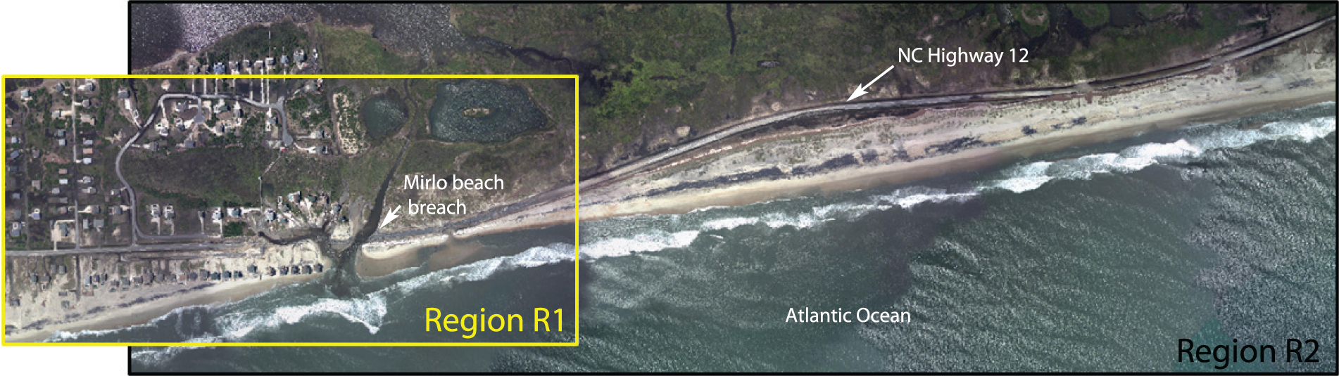
Aerial photography of the North Carolina Outer Banks shows study region R near the town of Rodanthe taken in August 2011, after Hurricane Irene. The two-pronged forked shape on Mirlo Beach in Region R1 is hurricane damage that breached the highway blocking access to the mainland.

Region C, near Cape Hatteras, is the southernmost tip of a bend in Hatteras Island (see Figure 2). The cape is a piece of land that protrudes at this elbow where warm Gulf Stream currents meet cold currents from the north and cause offshore turbulence. Cape Hatteras is frequently struck by hurricanes, including Hurricane Isabel that breached Highway 12 near Region C in 2003. The cape belongs to the Cape Hatteras National Seashore National Park, which draws over 2 million visitors annually.

Figure 2.

North Carolina Outer Banks and location of study regions.

Region J, within the Jockey’s Ridge State Park, features large dune fields, including one of the largest active sand dunes on the Atlantic coast of the United States. Since 1950, the main peak of the dune field has lost half of its height (from 40 to 20 m elevation) as the dune field migrated south at the rate of 3–6 m per year. Understanding of dune migration and transformation is important for its management and preservation as a unique landform feature and major tourist attraction with over 1.5 million visitors in 2011.

Data sources and processing

We explore the coastal terrain evolution using time series of elevation data for time periods of 1997–2011 in Regions R1 and C, 1996–2009 in Region R2, and 1974–2008 in the sand dune field Region J.

Elevation data

We demonstrate our visualization techniques using DEMs of the Outer Banks derived from geographically registered elevation data acquired by LiDAR (Table 1). (The day of the month of the February 2001 survey is unknown. February 1 was used in lieu of actual date.) An exception is Region J, where we used digitized contours to generate DEMs for the years 1974, 1995, and 1998. We acquired the LiDAR data from Digital Coast, a distribution site managed by the National Oceanic and Atmospheric Administration (NOAA) Coastal Services Center.²¹ Due to development in LiDAR technology during the study period and the fact that many of the LiDAR surveys were performed by different agencies, the multitemporal LiDAR dataset was diverse, creating resolution and accuracy issues that needed to be addressed.

Table 1.

LiDAR data sources include the USGS, the NASA, the NOAA (ALACE), the NCFMP, the USACE, and NGS.

Date	Name	Organization	Note
16 October 1996	Fall East Coast LiDAR	USGS/NASA/NOAA (ALACE)
2 October 1997	Fall East Coast LiDAR	USGS/NASA/NOAA (ALACE)
7 September 1998	Fall East Coast LiDAR	USGS/NASA/NOAA (ALACE)
9 September 1999	Fall East Coast LiDAR	USGS/NASA/NOAA (ALACE)	Post Hurricane Dennis
18 September 1999	Fall East Coast LiDAR	USGS/NASA/NOAA (ALACE)	Post Hurricane Floyd
February 2001	NC Floodplain Mapping Program	NCFMP
16 and 21 September 2003	Fall East Coast LiDAR	NASA/USGS	Pre- and Post Hurricane Isabel
25 July 2004	Topo/Bathy LiDAR	USACE
26 November 2005	Topo/Bathy LiDAR	USACE
27 March 2008	NGS North Carolina LiDAR	NOAA (IOCM)
1 December 2009	USGS Coastal LiDAR, North Carolina	USGS (EAARL)/NASA/NPS	Post Storm Ida
29 August 2011	NGS North Carolina LiDAR	NOAA	Post Hurricane Irene

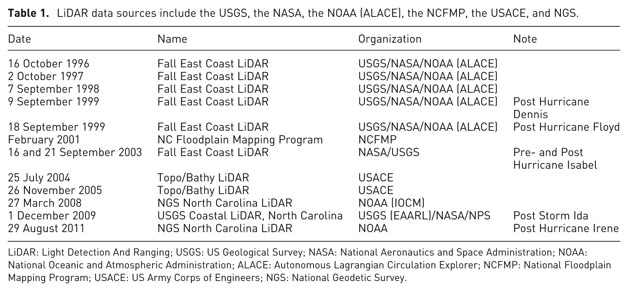
LiDAR: Light Detection And Ranging; USGS: US Geological Survey; NASA: National Aeronautics and Space Administration; NOAA: National Oceanic and Atmospheric Administration; ALACE: Autonomous Lagrangian Circulation Explorer; NCFMP: National Floodplain Mapping Program; USACE: US Army Corps of Engineers; NGS: National Geodetic Survey.

We first analyzed each LiDAR (x, y, z) point cloud to determine its spatial extent and point density and then interpolated at a 0.5-m resolution to create a DEM masked to a common region. The resolution is chosen by calculating the per-cell variability in the elevation of LiDAR points at a hierarchical set of resolutions and choosing the largest resolution such that the mean per-cell elevation variability is less than the published vertical accuracy of the LiDAR. This choice of resolution resolves important features, such as buildings, that were captured in the LiDAR. Next, we computed DEMs while simultaneously smoothing noise using regularized splines with tension.² For the purpose of correcting systematic error, the elevation differences between each DEM and geodetic benchmarks along North Carolina Highway 12 were estimated, and a constant elevation shift was applied to each DEM such that the median error became zero.²² We processed the DEMs for the sand dune field in Region J using the same general workflow at a 1-m resolution. We then used the resulting time series of DEMs to derive point and line features and raster map layers for visual geoanalytics. We also used a set of shore-perpendicular transects generated at 50-m intervals to sample ridge lines and compute longshore measures such as volume.

Features and summaries derived from elevation data

To characterize land surface dynamics, we use the multidimensional framework outlined by Mitasova et al.¹⁰ The framework integrates three approaches: feature evolution, surface evolution, and STC voxel models.

Feature evolution extracts topographic point and line features from DEMs for each time step and derives dynamic metrics such as rate of feature migration or elevation change. We use dune ridge, dune toe, and shoreline (Figure 3) represented as lines and discrete points for analytics of Regions R. We extract ridge line and toe line from the DEMs using the least-cost path approach developed by Hardin et al.²³ We generate the ridge line points at the intersections of the dune ridge line and a set of shore-perpendicular transects generated at 50-m intervals (Figure 3). Transects of 50 m were used here to be consistent with the US Geological Survey (USGS) National Assessment of Shoreline Change.²⁴ Ridge line elevation and migration is an important factor in determining vulnerability to storm surge and flooding. When very low elevations are registered, this can indicate a break in the ridge, which can result in flood damage to homes and roads. We generate shorelines as elevation isolines at elevation values close to the mean high water (MHW) level. Shoreline migration reflects short-term and long-term erosion and accretion trends due to sand redistribution and transport. To assess redistribution of sand over the study period, we used the 50-m transects to define polygons for volume change analysis.

Figure 3.

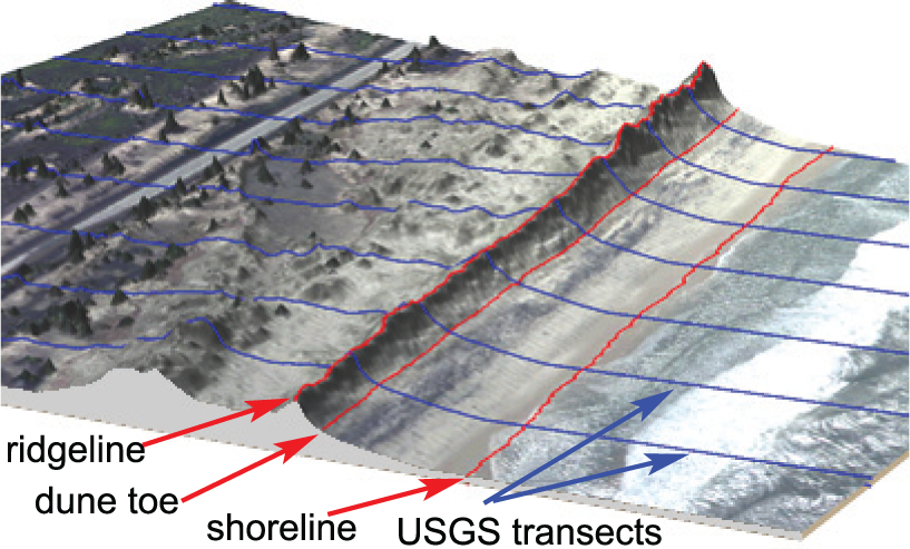
Dune features, ridge and toe, shoreline, and USGS transects perpendicular to shoreline.

We derive surface evolution metrics by applying per-cell statistical analysis to a time series of raster DEMs, resulting in new raster map layers that summarize the terrain evolution. We calculate the minimum elevation measured at each cell during the given time period to build a core surface and maximum elevation at each cell to create an envelope surface, so that the terrain is bounded within these two conceptual surfaces during the given time. We also derive maps representing the time of elevation minimum and maximum, as well as a number of additional statistical measures such as range and standard deviation in elevation and regression slope and offset.²⁵ We delineate a shoreface area called a shoreline migration band, the area between the MHW contours of the core and envelope surfaces. This area bounds shoreline evolution over the study period, and the width of this shoreline band is a measure of the magnitude of shoreline variability throughout the study period. Here, we use the core and envelope surfaces to derive relative volumes, which provide insight into sand redistribution over time within the shoreline band area and inland of the core shoreline.

Volume is measured within each 50-m segment and for each LiDAR survey so that both spatial and temporal trends can be observed. We measured volume evolution within the shoreline migration band and in the area that extends 110 m inland from the core shoreline. We then use relative volumes in the evolution analysis. We calculate relative volume in the area inland from the core shoreline for each segment $j$ as follows

{\hat{V}}_{i j} = \frac{V_{i j} - V_{c j}}{V_{e j} - V_{c j}}

(1)

where ${\hat{V}}_{ij}$ is the relative volume for the $i th$ LiDAR survey, $V_{ij}$ is the volume under the $i th$ elevation surface in the time series, $V_{ej}$ is the volume under the envelope surface, and $V_{cj}$ is the volume under the core surface. The volumes are calculated relative to MHW. Equation (1) essentially provides a normalization of the volume relative to the core and envelope surfaces for each land segment at each time step. Volume is also measured within the shoreline band (area between the core and envelope shorelines). The relative volume within the shoreline band is computed for each segment $j$ as

{\hat{W}}_{ij} = \frac{W_{ij}}{W_{ej}}

(2)

where ${\hat{W}}_{ij}$ is the relative volume for the $i th$ LiDAR survey in the time series, $W_{ij}$ is the volume under the $i th$ elevation surface in the time series, and $W_{ej}$ is the volume under the envelope surface within the shoreline band. By definition, the core surface does not exist within the shoreline band above MHW, and therefore, the core volume $W_{cj}$ is equal to zero. Although most of the previous research on volume change uses absolute values of volume,^1,3 analyzing and visualizing the volume data as relative volumes offers some advantages: Removal of the core values from the analysis highlights changes, such as sediment transport in areas where the volume of transported sediment is much less than the volume of the stable sediment under the core surface. Because the core represents a minimum bound on volume and shoreline evolution, values from the core represent worst-case scenarios observed in the time series. Because terrain evolves exclusively within the dynamic layer, visualizing volume as a percent of the dynamic layer volume and shoreline band area allows for the at-a-glance determination of the present state relative to the minimum and maximum observed over the study period.

Elevation voxel models for STC

To capture elevation dynamics in a continuous space–time domain, we compute and analyze it as a trivariate function represented by a space–time voxel model. Time series of LiDAR data include massive point clouds with varied point density and sampling patterns. Heterogeneity in LiDAR point cloud data acquired over the past decade is due to the rapid evolution of LiDAR mapping technologies, the different objectives of individual surveys, and the spatial coverage that may not be complete for all surveys, creating additional gaps in the time series. Computation of a space–time model of terrain evolution from massive, noisy point data, heterogeneously distributed over space and time, is therefore nontrivial. We use two approaches to create the voxel model of terrain evolution. The first approach performs the data integration (georeferencing, detection, and removal of systematic errors; masking to a common spatial extent; and interpolation to a common resolution and level of detail) in 2D resulting in a consistent series of DEMs. These DEMs are then stacked to create a voxel model, where each vertical level of the voxel model is associated with time of the DEM survey. For surveys performed at equal time intervals, the vertical resolution of the voxel model represents a rescaled time interval. If the surveys were taken at irregular time intervals and the time interval is highly variable (e.g. days between some surveys vs years between others), each vertical level has the time interval stored as an attribute, which can be used to assign colors that reflect the variable time. The second approach described by Mitasova et al.¹⁰ creates the voxel model directly by trivariate interpolation of time series of point clouds. The STC creates a voxel representation of elevation evolution with time as the third dimension and elevation as the modeled variable. Once a voxel model is created, the evolution of contour-based features, such as shorelines, can then be represented by isosurfaces.

Socioeconomic data

Tourism draws millions of vacationers to the Outer Banks each year providing a major source of income in this region. Since the islands of the Outer Banks are isolated with limited access by road, breaches in the highway may affect development.

In coastal regions with extensive development and frequent severe storms, home construction and destruction exhibit significant activity even at the decadal scale of the study period. New or lost buildings can be efficiently identified from a time series of high-resolution DEMs using grid cell comparisons. Cells in which differences between the core and envelope exceed a given threshold are identified, and the time of minimum and maximum elevations is compared for these cells (see Mitasova et al.²⁵ for more details). Additional information about the timing and spatial pattern of new home construction and loss or relocation of homes can be provided using the voxel elevation models as STC. We extracted elevation isosurfaces associated with the building height from the voxel models and colored them by the year. The location and topology of these isosurfaces then provide information about the time and location of new construction, loss of a building, or its renewal.

Visualization design

Designing visualizations to support sensemaking in geomorphology requires a knowledge of the target audience and the application requirements. Here, we are considering the changing landscape of the sandy barrier islands of the North Carolina Outer Banks. As discussed earlier, this area is frequently impacted by large storms, such as hurricanes, tropical storms, and large storms called nor’easters. The most recent LiDAR survey along the Outer Banks was taken in August 2011, following Hurricane Irene, after several breaches formed along North Carolina Highway 12. Several other of the LiDAR surveys were collected post storm as well: post Dennis and post Floyd (1999), post Isabel (2003), and post nor’easter Ida (2009). While we expect to see dramatic changes after these events, other natural processes such as wind and wave transport can cause more gradual landscape changes. Anthropogenic activity also causes the natural and built landscape to change. In some locations, the severely eroded beaches are rebuilt by beach nourishment or sand disposal. Diverse groups such as the general public, decision makers, and civil engineers have a need to understand some aspects of these processes. However, our focus in this work is to enable domain experts—coastal scientists—to explore these phenomena. For this kind of analysis, we can characterize a core task set as follows.

Explore the dynamic nature of the landscape over time.

Keep the geographic context while studying the data.

Keep the temporal context of irregular time intervals in available data.

Identify significant changes in coastal topography, such as dune ridge height decrease, volume change from sediment displacement, and shoreline migration.

Find signs of a region’s vulnerability to storm impacts, such as overall decreasing dune heights, landward migration of shoreline, and coastline breaching.

Identify landform trends, not just changes between pairs of time steps but also longer term change patterns.

Inspect the construction and loss of built features in the context of time.

These goals present a formidable visualization challenge, given the complexity of the processes involved in landscape changes. Standard GIS approaches to visual analysis of coastal geomorphology consist of small multiples for side-by-side comparison of 2D snapshots in time and contour lines to represent linear features to show changes in attributes such as beach area and shoreline.²⁶ As the number of time steps increases, comparing surveys becomes more difficult using these approaches. Animations are also commonly used to show spatial changes over time.²⁷ The differences between frames in an animation draw attention to the changes that occur over the area.²⁸ However, the limitations in visual attention make it difficult to compare trends within the study area. Multitemporal datasets sampled at uneven time intervals introduce additional stumbling blocks to these techniques.

Studying the evolution of landforms requires the ability to search for trends over multiple time steps. With this in mind, we look at ways of displaying multiple time steps within a single image. Because of the volumetric nature of our datasets, we look to existing techniques for incorporating time as a spatial axis, and we apply them in a way that supports analysis of complex terrain evolution processes. Several visualization principles including the following were used to achieve this.

Perception-based selection of salient visual features. The visualizations should employ rapidly perceptible visual texture features such as color, shape, and size.

Selective data reduction so that high-priority data components (such as the temporal dimension) are incorporated. The system should highlight data aspects of particular interest, such as the lateral and vertical movements of dune ridges or the migration of the shoreline.

Making use of human interaction as part of an exploratory process. The user should be able to interactively explore the data, not only through standard scene navigation tools but also by modifying key attributes being inspected to vary the data views.

We designed our STR, STC glyphs, and STC isosurface data views employing these principles: These views use salient visual features—color, texture, shape, and size—and employ color schemes that are consistent with the nature of the underlying data being derived from perceptive color models.^29,30 Additionally, the STR follows the USGS convention of referencing positions based on longshore distance, a measure of distance along the coast, taking advantage of the linear nature of the geography to reduce the data complexity. The data represented by STC glyphs represent data reduction in terms of summarization or feature extraction. The isosurfaces reduce the complexity of the data by fixing the elevation within a space–time voxel. Furthermore, the user can interactively explore the data using each of these techniques by varying a component of what is being visualized. We demonstrate the user exploration process and the support of sensemaking by presenting our data views of real-world data in section “Visualization methods and results.”

Visualization methods and results

We present a set of visualizations that provide a unique insight into the spatial and temporal patterns and relationships of dynamic coastal features, surfaces, and volumes using glyph-based STC approaches, heat graphs displayed in STR, and STC isosurface renderings. The visualizations are developed using open-source GRASS GIS surface and volume modeling and visualization modules and custom code modules based on OpenGL libraries.

Terrain feature evolution

We can represent linear features that characterize the coastal landscape, such as dune ridge, dune toe, and shoreline by sampling the lines at regular intervals so that these features can be displayed as discrete glyphs in an STC model. Figure 4 illustrates this approach for a dune’s ridge line in Region R1.

Figure 4.

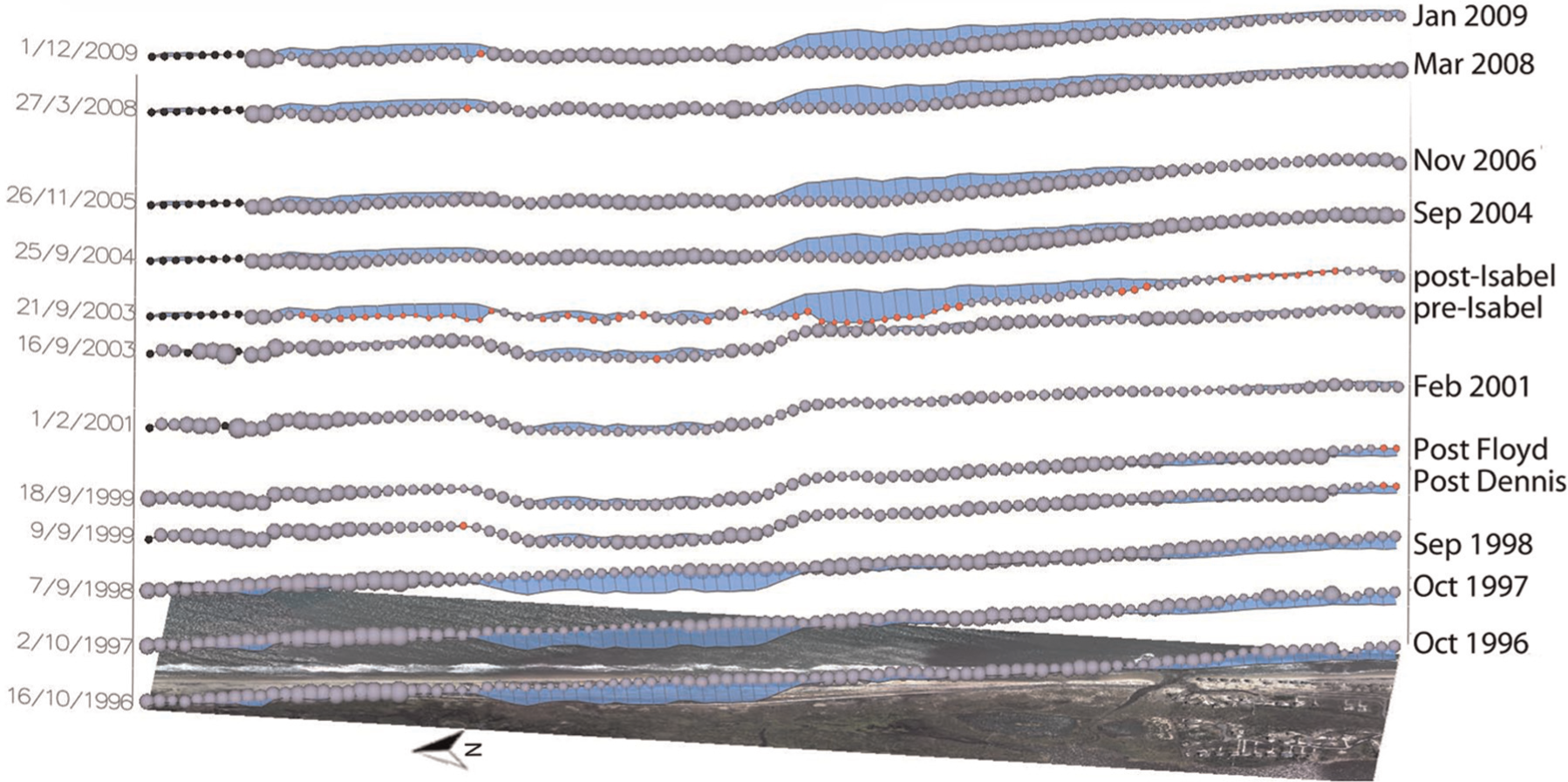
Space–time cube visualization of Rodanthe ridge line elevations for Region R2. Sphere size indicates elevation (purple for 3.01–8.19 m, red < 3 m, black = no data). Blue fins (parallel to the ground plane) show the magnitude and direction of the ridge line from median ridge line position at that location. Hurricane Isabel breached the dunes in 2003 (red spheres).

The glyph-based approach shown in Figure 4 represents elevation of points sampled at 50-m intervals along the foredune ridge lines. In the figure, spheres are displayed at intersection points of transects and ridge line; size of the spheres encodes magnitude of ridge line elevation. Additionally, we use red spheres to mark locations where there was loss of foredune (i.e. elevation less than 3 m). Many sample points on this ridge line dipped below 3 m after Hurricane Isabel. A glyph-based STC allows us to represent other information such as magnitude and direction of migration of a ridge line and changes relative to previous years.²⁰ The median ridge line in the figure was computed based on elevations or ridge line for a given transect for every time step. Deviation of a ridge line for a given time step from the median ridge line is shown using blue “fins” that are parallel to the ground plane. This visualization shows not only patterns of changes in the temporal dimension (elevation magnitude changes) but also local spatial changes (migration of dune ridge relative to the median). For example, in this visualization, we can see that a portion of the ridge line just north of Mirlo Beach retreated inland from the median position in the years following Hurricane Isabel through 2009.

Figure 5 uses elevation as the vertical axis to display a 3D scatterplot of elevations in Region R2. Time is encoded implicitly using a salient graphical property, glyph color. Although simple, this technique provides an informative view to explore patterns of elevation changes along a ridge line. Time steps can be highlighted interactively, enabling comparisons such as pre- and poststorm ridge line elevations. The poststorm band of glyphs seems to portray a pattern that is distinct from the prestorm pattern, particularly in the northern portion. This approach highlights the loss of dune elevation after Hurricane Isabel, but does not show the horizontal migration of the ridge line.

Figure 5.

A three-dimensional scatterplot showing clusters of ridge line elevations for Region R2. The vertical axis represents elevation scale and time is represented using color. Glyphs (spheres) are colored by three distinct colors for three time intervals that correspond to time steps before, during, and after Hurricane Isabel in 2003 (see color scale). Elevation values for the 21 September 2003 survey (just after Hurricane Isabel) are highlighted in the figure.

Additionally, the temporal evolution of the dune ridge can be summarized by a heat graph showing evolution of minimum dune height within each 50-m segment (see Figure 6(a)). Figure 6 employs only longshore distance to locate dune height and volume, not the land extent of the dune. Focusing on the longshore value of attributes provides a data reduction, so that STR can be used along a reference DEM (Figure 6(a)-top). The height of the rectangles vary based on the time intervals, meaning that surveys that were only days apart, such as the pre- and post-Isabel surveys appear as lines. This creates the sharp transitions that emphasize rapid change events.

Figure 6.

Derived coastal properties for a 5-km strip including Region R2. (a) DEM of Region R2 (top) and dune height heat map showing the evolution of minimum dune and berm height (bottom). (b) Core/envelope volume plot (top) showing segment-based volume evolution for the subarea inland from the core shoreline. Solid line -> volume under the core surface; Dashed line -> volume under the envelope surface. Evolution of the inland relative volumes represented by color (bottom). Values close to zero indicate volume close to core (minimum). Values close to one indicate volumes close to the envelope (maximum). (c) Shoreline band volume: Segment-based volume evolution analysis for the subarea within the shoreline band. Evolution of the relative volume shows close to core values for the post-Hurricane Dennis and Isabel surveys.

Sand mass redistribution

The user can interactively explore the data by modifying the attribute being visualized in the STR. Changes in dune ridge height indicates sand volume redistribution and transport. The first relative volume STR Figure 6(b) provides information on the status of volume $V_{ij}$ at time $i$ in the segment $j$ in relation to volume maxima (envelope volume) and minima (core volume) in the segments inland of core shoreline. Figure 6(b) shows that the northern 500 m (segments 375–385) of the area has experienced loss in the sand volume, which is likely due to Hurricane Isabel, where the relative volume transitioned from the high, near-envelope value (dark blue) in 2001 to the low, near-core value (dark red) in 2008. The southern section (segments 390–465) gained volume during the study period, with most of this area having a relative volume of about 20% of the dynamic layer volume from 1996 to 1999 and volumes near 60% of the dynamic layer after 2001. Throughout the area, 2001 had the greatest volume.

Figure 6(c) shows the variation in the volume bound by the MHW and the envelope surface, there is no core surface above MHW within the shoreline band. The influence of extreme events can be easily identified in the graph that shows spatial and temporal variability in the relative volumes (Figure 6(c)). Substantial loss of volume occurred during the years 1999 and 2003 due to Hurricanes Dennis and Isabel, when volumes changed from near-envelope (close to 1) to near-core (close to 0).

Diverging red–blue color schemes²⁹ are used for the STR in Figure 6(b) and (c) with the break point relative volume of 0.5, halfway between core and envelope, colored white. This enables the viewer to quickly perceive when the relative volume is close to core (dark red) versus envelope (dark blue). The red–blue color scheme was chosen for Figure 6(a) as well for consistency with other STR and with the glyph-based STC so that the lower half of the dune height observations is red with the white transition at the median dune height of about 3.4 m.

The examples in Figures 4 –6 show that the STR and glyph-based STC data views are designed to facilitate studying trends by combining multiple time steps within each individual representation of the attributes under consideration. A single carefully designed view can provide a more effortless environment for trend analysis than conventional multiple coordinated DEMs or looping animations.

Terrain surface evolution

We stacked DEMs in an STC to create a voxel model of terrain evolution in Rodanthe (Region R), Cape Hatteras (Region C), and Jockey’s Ridge (Region J) areas to demonstrate insights that this approach can provide for landscapes that are evolving due to geomorphic processes. We extract an isosurface for a selected elevation value to represent terrain evolution along this elevation contour. We can then associate the topology of the isosurface with the underlying geomorphic processes. To enhance interpretation of such isosurfaces, we drape a color map over the isosurface to associate the stratum of the isosurface with the epoch (time period). For epoch-based coloring, we select time step colors with colors chosen to reflect the difference in time between the surveys using Healey’s³⁰ perceptually balanced color scheme. This technique for choosing effective colors for data visualization provides a mapping for the distance between attribute values to perceived distance between colors. Alternatively, other attributes, such as the rate of change (Figure 7(b)) or distance to a road, can also be represented by draped color map.

Figure 7.

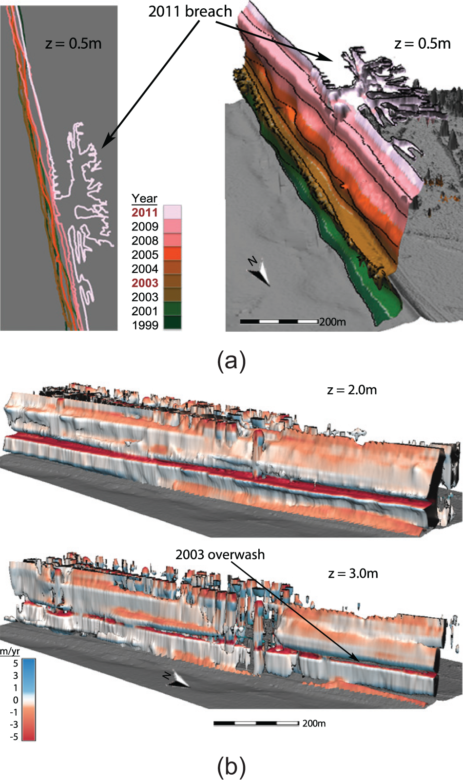
Region R terrain evolution. (a) Shoreline contour lines (left) and isosurface contours (right) extracted at 0.5 m and colored by year. Both images show the massive overwash as a result of Hurricane Irene in 2011. (b) Isosurfaces extracted at 2- and 3-m elevation colored by rate of elevation change in meters per year. High rate of loss (red) is associated with the impact of Hurricane Isabel in 2003.

Evolution of the Mirlo Beach location in Rodanthe is influenced by coastal erosion due to waves and storm surges and anthropogenic activities that include beach and dune restoration and stabilization. Coastal dynamics are measured by analyzing the migration of shoreline commonly represented by a MHW contour. In some coastal applications, linear features such as shorelines are displayed using contour lines.²⁶ However, this approach breaks down quickly when the number of lines increases and begins to cross. Even though they are displayed using a perceptual color scheme based on time step intervals, the Region R shoreline contours, when displayed in 2D result in a tangle of lines that is quite difficult to decipher (Figure 7(a)). As an alternative to these overlapping lines, the shoreline can be extracted from the voxel model to create an isosurface representing shoreline elevation. This creates a kind of extruded surface where changes in the shoreline become much easier to compare. In Figure 7(a), we used an elevation of 0.5 m to generate a Rodanthe (Region R1) shoreline isosurface using the same color scheme applied to the contour lines. The black line drawn passing through the center of each interior color band on the isosurface represents the shorelines for each time step. The bottom and top color bands terminate at the first and last surveys, respectively. The vertical distance between the shoreline bands represents the epoch length. The position of the isosurface is interpolated between these lines. Stretching the shorelines with a vertical time axis highlights the repeated pattern of shoreline advance and retreat (as the isosurface undulates through time) and the dramatic intrusion of shoreline inland due to the breach caused by the 2011 hurricane. Color and draped shorelines help to associate the time with specific shoreline geometry and its evolution. Evolution of upper beach or lower section of the foredune can be represented by 2-m isosurface.

The user can interact with this data view to explore the data, by changing selected elevation and color scheme. Figure 7(b) shows the same site, Region R at different elevations with a different color scheme, providing additional information about Region R. The coloring reflects the rate of elevation change per time step instead of the epoch, which is still mapped to the z-axis. A red–blue diverging color scheme emphasizes the difference between sand gain and loss. Figure 7(b)-top shows the sudden retreat due to Hurricane Isabel in 2003, followed by recovery and gradual retreat in the years 2008–2011, creating conditions for the 2011 breach in Region R1. Both 0.5- and 2-m isosurfaces for Region R1 are continuous, indicating that except for the breach, elevation in this location was never lower than 2 m. The 3-m isosurface (Figure 7(b)-bottom) shows a large opening in 2003. This was apparently overwash due to Hurricane Isabel, which temporarily reduced the elevations in this location to less than 3 m.

Applying the isosurface view to a different location, Region C, we can observe different kinds of patterns. Evolution in the Cape Hatteras area is driven by ocean currents, storm surge, and wave action. These conditions lead to significant sand transport with complex patterns. The shoreline evolution isosurface (Figure 8(c)) that reveals the changes in the shoreline involve the retreat and regrowth of the cape tip along with changes in its direction. The surface is again colored by epoch so that the year associated with each phenomenon, such as maximum retreat, can be identified using the color draped over the isosurface. These types of patterns are much more difficult to decipher in the corresponding shoreline contour line representation shown on the left.

Figure 8.

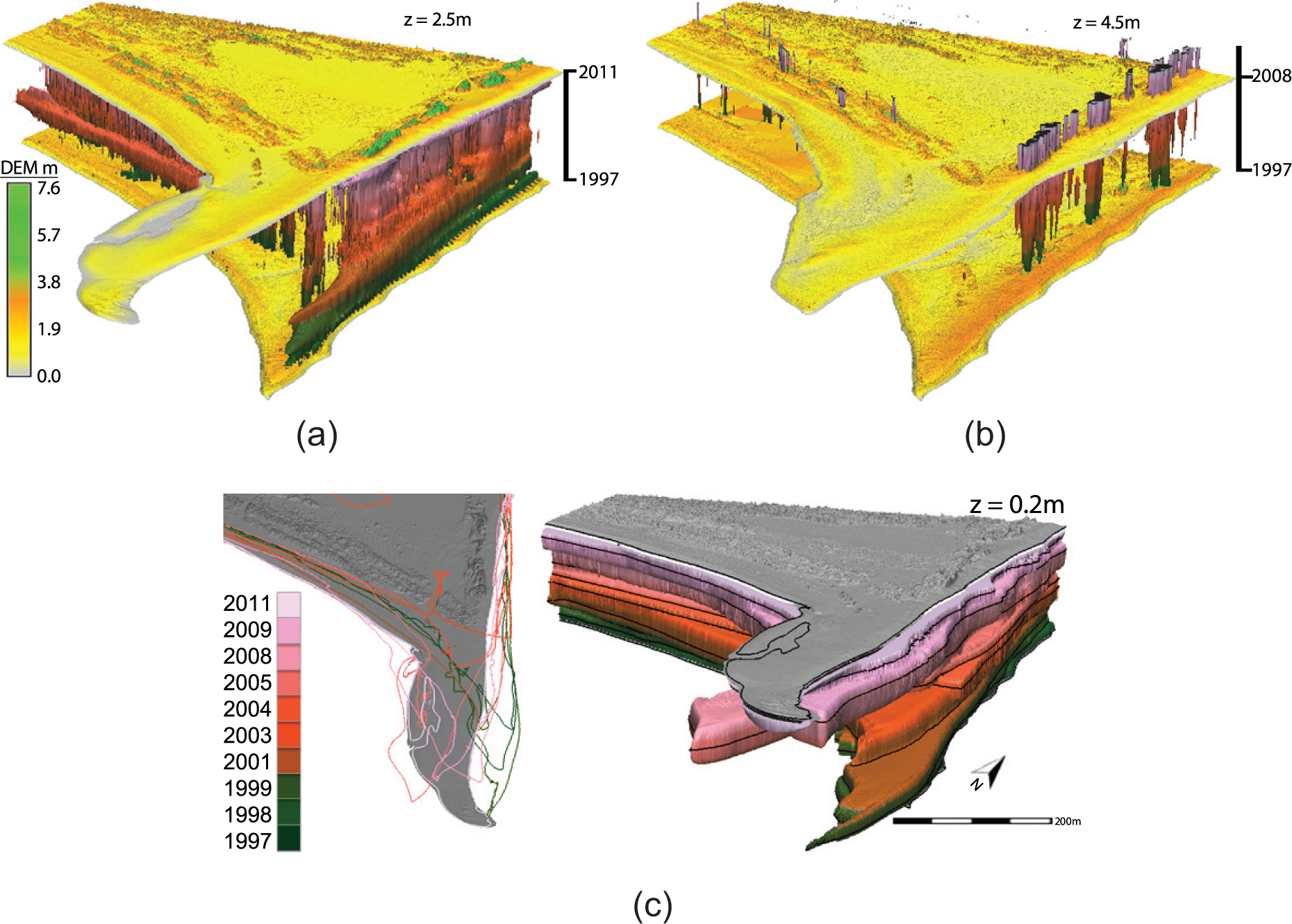
Region C, Cape Hatteras terrain evolution. (a) 2.5-m elevation isosurfaces sandwiched between the 1997 and 2011 DEMs at their temporal locations. (b) 4.5-m isosurface shown with 1997 and 2008 DEMs at their temporal locations. (c) Shoreline contours (left) and shoreline 0.2-m elevation isosurface (right) displayed with the 2011 DEMs in gray.

We also use Region C to demonstrate a different isosurface technique, which sandwiches an isosurface between DEMs. Evolution of the mid-level and top of the dunes is represented by isosurfaces with elevations of 2.5 and 4.5 m (Figure 8(a) and (b)). The related DEMs positioned at their respective time coordinates in the STC associate the contour with its position in the surrounding landscape at the given time. In Figure 8(a), DEMs for the first and last surveys (1997 and 2011) are shown. The user can also select other DEM pairs. For example, the 4.5-m isosurface in Figure 8(b) uses the 2008 DEM along with the 1997 DEM. These sliding DEMs provide additional context for the change patterns. For example, in most places, the dunes on the eastern coast of Region C that had formed as of 2008 retained at least a 4.5-m elevation, as there is very little deterioration in the column-like shapes that formed below that level. Also, no large new dunes grew above 4.5 m after 2008, all extruded columns begin below that DEM.

We visualize longer term evolution of dunes, driven by eolian sand transport, for the Jockey’s Ridge dune field (Region J). The migration and transformation of the dune field between the years 1974 and 2008 has been visualized and analyzed in previous works using several standard techniques, such as animations, cross-sections, core and envelope summaries, and peak and crest feature position overlays.²Figure 9(a) shows 1974, 1999, and 2008 DEMs of Region J. These show that the peaks lost height and the higher dune split into several ridges. This is useful information, but we want to know more about the transformation of the dune form. To provide insight into the transformation of the large dune from a 40-m-high dune with single peak into several 20-m-high parallel ridges, we use a stacked voxel model created from seven DEMs spanning the years 1997–2008. We extract isosurfaces for the elevations that define the dynamic section of the dune at 17, 20, 21, and 15 m and assign them colors that identify the epochs associated with levels of the isosurface—assigning colors that represent the interval jumps with appropriate color distances is especially important here because the time intervals are highly irregular.

Figure 9.

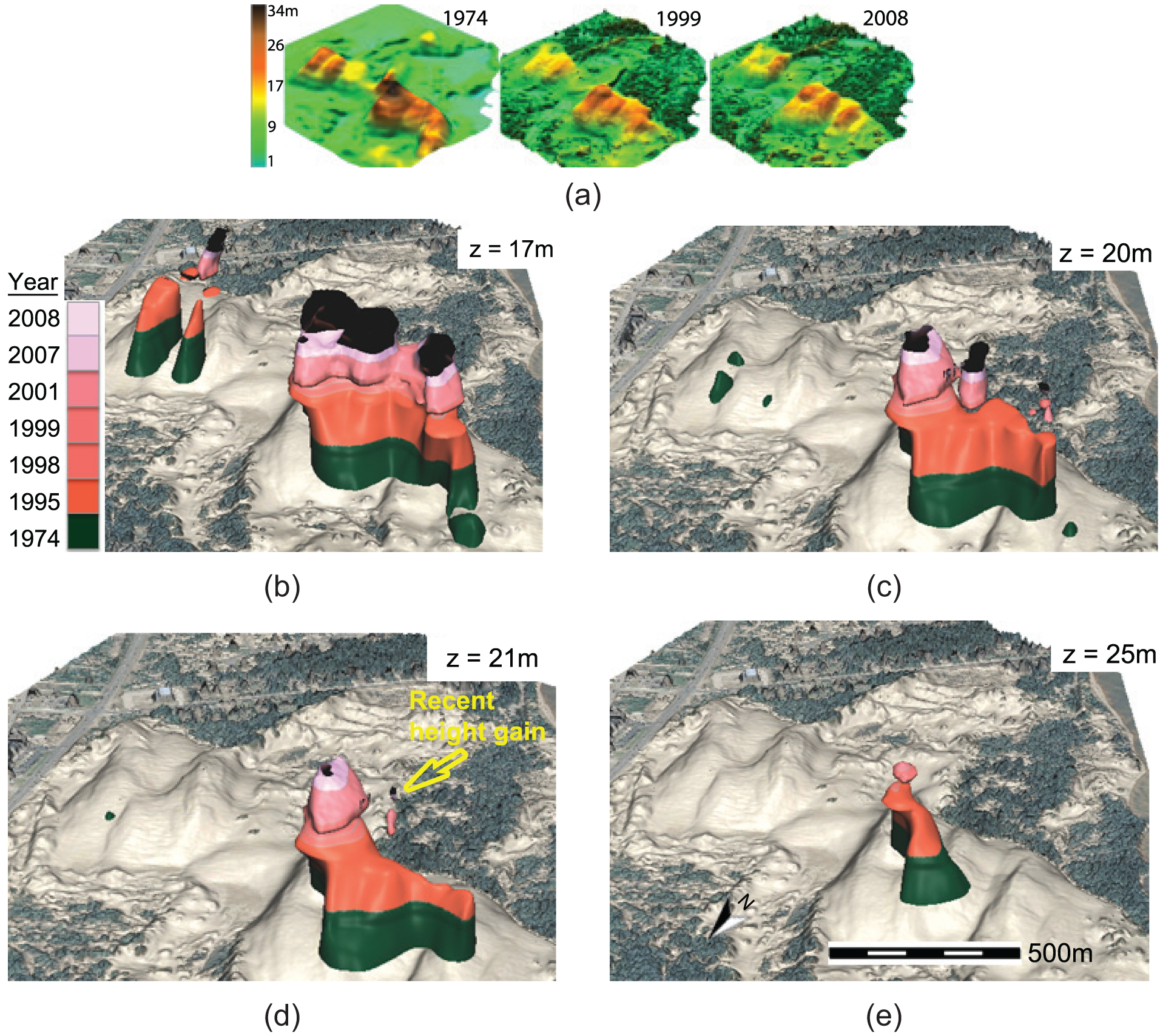
Evolution of a Jockey’s Ridge dune field (Region J) and its transformation to parallel ridges: (a) 3D view of 1974, 1999, and 2008 DEMs and evolution of (b) 17-m, (c) 20-m, (d) 21-m, and (e) 25-m contours showing the formation of separate ridges at different elevation levels, decrease in main dune elevation, and growth in west ridges.

The 17-m isosurface (Figure 9(b)) clearly shows the evolution of three distinct ridges since 1995, as shown by the emergence of three chimney-like forms. The 2008 color still appears in Figure 9(c), meaning the main dune stayed 20 m high at all times, although, over the last 2 years, the 20 m area narrowed substantially. The area west of the main dune lost elevation, going below 20 m in the period after 1974 but gained the height again in 2007 at two distinct, parallel ridges (as shown by the floating chimneys in Figure 9(c)). The 21 m peak of main dune disappeared in 2007, but the dune has regrown to this height recently at a small spot west of the main dune (marked in Figure 9(d)). The 25-m isosurface, Figure 9(e), shows the narrowing of this elevation as it moved south east, disappearing after 2001. Enabling the user to interactively explore isosurface elevation values in this way facilitates a much more detailed understanding of this phenomenon than a DEM comparison.

Anthropogenic activity

We can also visualize spatial–temporal change caused by human activity to investigate spatial and temporal patterns of the socioeconomic impact of storm damage. One interesting aspect of socioeconomic data is the construction and loss of buildings, usually homes built close to the shoreline. For this discussion, we return to the same region we analyzed in Figure 7. Where our previous discussion focused on shoreline variability and sand accretion and loss, the same piece of land also has intensive anthropogenic activity, as this is beachfront property in a popular summer resort town. Figure 10 illustrates this phenomenon in Rodanthe Region R1, using several different approaches. We created Figure 10(a) using map algebra techniques described in the study by Mitasova et al.,²⁵ which use the difference between the core and envelope surfaces combined with the time of minimum and time of maximum maps to identify the homes constructed or lost during the study period. The cells with lost or built status during the years of 1999–2011 are marked in red and blue, respectively, on a 2011 DEM in Figure 10(a). Transect 4 passes through one home that was built, one that remained the same, and one that was lost (Home A). Aerial photographs of 1998 and 2011 in Figure 10(b) and (c), respectively, show the same locations with Home A appearing in Figure 10(b) but not in Figure 10(c). Figure 10(d) shows a profile of the core (red) and envelope (green) surfaces at Transect 4. The terrain variations between the core and envelope are shown in grayish green. The envelope is much taller than the core where a home was built (left) or lost (Home A). The core rises to meet the envelope for the home that remain unchanged (the small bump between the built and lost homes).

Figure 10.

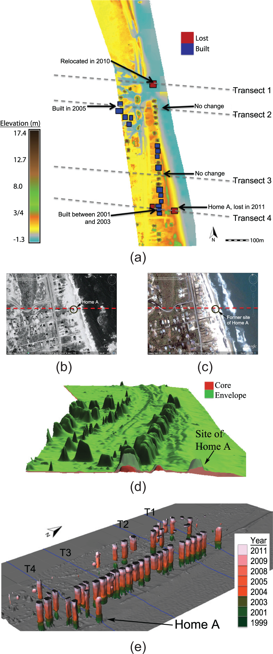
Region R1 home loss and construction analysis during 1997–2011. (a) 2011 Region R1 DEM with loss/construction marked. (b) and (c) Imagery from 1998 and 2011. (d) Core and envelope profile at Transect 4. (e) Homes appear as columns in the isosurface contours at 6 m. Home A column has a rounded red cap due to its 2011 destruction.

Finally, Figure 10(d) shows that in addition to beach and dune topography, higher elevation isosurfaces (in our case 8 m) offer information about home construction and destruction. Figure 10(e) demonstrates this for homes in Rodanthe in Region R1. Homes are stable, so the isosurfaces of homes appear as vertical columns, but the vertical extent of the columns indicates when they were built or lost. Floating columns represent homes that were constructed or reconstructed during the time period. Columns with an open top indicate that the home remained standing at the time of the last LiDAR survey; homes with a rounded cap did not. For example, Home A was destroyed in a hurricane in 2011. This isosurface provides valuable temporal information about the changes that is not available in a DEM display such as Figure 10(a).

Discussion

Figures 4 –10 provide insightful analyses on coastal terrain evolution along the North Carolina Outer Banks. With STRs, we were able to view extracted features in 2D format; with glyph-based STC, we were able to view extracted features within the geographic context; and with isosurfaces, we were able to view extracted features in an abstract spatial format. We demonstrated STRs on minimum dune height, inland relative volume inland, and shoreband relative volume; we demonstrated glyphs on dune ridge elevation and the glyph-based STC on dune ridge elevation and lateral position; and finally, we demonstrated STC isosurfaces on shoreline, low-dune, mid-dune, and high-dune elevations, as well as built features.

We saw abrupt changes within the Outer Banks (STRs post storms in Region R2, isosurfaces post storm in Region R1) as well as gradual long-term changes (isosurface high dune to lower ridges in Region J). We saw pattern shifts in important features (glyph STC dune ridge shift landward in Region R2, isosurface shoreline shift landward in Region R2 prior to the breach).

To evaluate the results of our case study, we return to the applications requirements identified in section “Visualization design.”

Explore the dynamic nature of the landscape over time. We selected data views with the constraint that multiple time steps be displayed in a single visualization. These techniques have a number of strength and weaknesses. The STR provides an at-a-glance attribute summary by juxtaposing time steps. A limitation of both the STR and STC isosurface approaches is that the values interpolated between surveys though the interim change patterns are unknown. A glyph-based approach holds an advantage in this sense, because each glyph represents a survey sample point.

Keep the geographic context while studying the data. Spatial context is important to domain experts studying the data who use this information to locate positions where important events have occurred. The STR is displayed along with a DEM to attach spatial context. The glyphs and the STC isosurface also allow the data to be displayed in situ to provide the geographic context where the events occurred. Also, the STR and isosurfaces can be adapted to visualize information for large spatial extents, for example, the north to south extent of the Outer Banks.

Keep the temporal context of irregular time intervals in available data. Our approach allows users to identify the temporal differences in consecutive time steps. We achieve this by careful design of a color mapping scheme and by explicitly displaying the differences in the time intervals between successive data gathering steps in the STR and STC.

Identify significant changes in coastal topography. The STR and STC revealed loss in dune ridge height as blue changes to red and the isosurfaces showed loss of dune height as pitting or holes in the surfaces. The STR revealed relative volume change from sediment displacement, the STC revealed dune ridge migration as deviations from a median ridge position and the isosurfaces revealed shoreline migration as undulating surfaces.

Find signs of a region’s vulnerability to storm impacts. We can see this in several of our examples. The STR revealed overall shoreband losses in volume after Hurricane Dennis. That portended the recurring loss after Hurricane Isabel. Figure 4 shows the receded dune ridge after Hurricane Isabel near where the 2011 breach would occur. The isosurface in Figure 7(a) shows that the shoreline in this position was also migrating landward, still losing sand even after sand was added.

Identify landscape trends, not just changes between pairs of time steps but also longer term change patterns. In addition to vulnerability patterns, our examples show other trends during the study period. Figure 4 shows patterns of advance and retreat of the ridge line. Figure 7(a) showed the landward movement of the shoreline after Hurricane Isabel in 2003. Figure 8 showed the western pull of sand in Region C. Figure 9 showed the change of a single tall dune into multiple lower ridges.

Inspect the construction and loss of built features in the context of time. The isosurface in Figure 10(e) shows a novel means for exploring this information. The isosurface used in this way is an abstraction of the information that the user at first may need some instruction to interpret. Once familiar though, this is a convenient shorthand for this information.

Comparing these analyses over several locations along the Outer Banks emphasizes coastal terrain evolution over a decadal time series. In Figures 3 –9, it is clear that major terrain changes, from the shoreline to the dune ridges, occurred after storm impacts. These visualizations not only show how storm impacts affected the terrain but also show how the terrain was rebuilt/recovered after these events. Using these techniques to visualize volume change, shoreline, and dune migration, as well as coastal development, enhances understanding of the changes over the time series. Visualization is a powerful tool for understanding how the coastal areas evolve, and using several approaches to quantify and visualize supports analysis of change over a dynamic region. In fact, visualization reveals the high spatial and temporal variability in terrain evolution, which may help to explain why the solutions to coastal management of this type of landscapes are so difficult and why it is so hard to find consensus.

We have shown how these techniques work well for study of coastal terrain. This may be partly due to the linear nature of many of the features of interest (shorelines, ridge lines). But this is a fairly common quality of landscape phenomenon (stream beds, streets, snow crests, etc.). These types of visualizations could also be applied to the study of other dynamic terrains, such as landslides, glaciers, snow cover, changing land cover, stream bed erosion (where erosion would be measured instead of elevation), or even scans of changing cityscapes, an area in which data collection is exploding.⁵

Conclusion

Coastal LiDAR data are being gathered at unprecedented rates and high resolutions. Traditional GIS-based approaches are not sufficient to explore complicated spatial–temporal changes that occur in highly dynamic environments. We have presented approaches based on STC geovisualization and other visualization techniques to explore coastal terrain dynamics in the North Carolina Outer Banks and investigated terrain features (such as dune ridge line position and height), terrain surfaces, and socioeconomic data. Several study regions were used to demonstrate the variety of trends revealed by these visualization techniques.

We can see the benefits of the visualization techniques shown in this work, when compared to the information provided by traditional techniques. The use of the STC, adding time as a third dimension, allows us to visualize changes in patterns, geometry of landform evolution. For example, tracing ridge line contours in two dimensions, a conventional technique for coastal linear features, such as shoreline, portrays the range of horizontal movement (Figure 7(a)-left), but adding a temporal component allows us to view temporal trends, such as the cyclic advance and retreat of a shoreline (Figure 7(a)-right). Although important events such as dune breach or overwash can be seen with conventional techniques, our approach presents them within a temporal context, revealing the terrain form before and after the event. This allows viewers to assess whether there were some features in the terrain that indicated vulnerability for a long time prior to the event or whether there was only a short-term vulnerability leading to the event. Similarly, conventional line graphs of coastal longshore properties such as sand volume, as a function of longshore distance, are less effective when multiple time steps are graphed together. Using a temporal axis to create STR heat graphs of sand mass volume change over time portrays trends in sand redistribution in a perceptually salient manner. Future work aims to find linkages between the spatiotemporal geometry and processes.

We adapted the standard STC to explore evolution of coastal features such as fore dunes. The STC is well suited in our work because it retains the spatial or geographic context while plotting temporal data. The different STC-based approaches that we have described, that is, glyph-based and isosurfaces, enable us to display important spatial information such as topographic or orthophotographic information, which provides important context and makes it easier to explore the terrain dynamics in our study regions. Moreover, our glyph-based visualization in the STC allows us to plot heterogeneous information and combine it with standard LiDAR-based data. In our results, the glyph-based STCs reveal lateral shift of foredune ridges and changes in foredune ridge height due to storms.

Our results reveal terrain changes of shoreline and dune ridge migration, dune breaches and overwash, the formation of new dune ridges, and the construction and destruction of homes, changes which are due to erosion and accretion, hurricanes, and human activities, including the vulnerability of built structures such as buildings and roads in this environment. A variety of visualization techniques were used to derive information from LiDAR to help scientists better understand how the system behaves, including the range of dynamics and which features are stable and which are unstable.

This work demonstrates these approaches on barrier islands in North Carolina, but application could be extended to other coastal terrains or other volatile terrain environments, such as landslides or stream bed erosion. For terrains such as these, a variety of views—visualization and analytic techniques—of time-series terrain data are needed in order to ascertain and interpret the nature of the terrain behavior over time.

Footnotes

Acknowledgements

The authors wish to thank NOAA Digital Coast for providing the LiDAR surveys.

Declaration of conflicting interests

The authors declare that there is no conflict of interest.

Funding

This work was supported in part by a grant W911NF-09-1-0560 from Army Research Office. This work was also supported in part by RENCI.

References

Burroughs

Tebbens

. Dune retreat and shoreline change on the outer banks of North Carolina. J Coastal Res 2008; 24: 104–112.

Mitasova

Overton

Harmon

. Geospatial analysis of a coastal sand dune field evolution: Jockey’s ridge, North Carolina. Geomorphology 2005; 72(14): 204–221.

White

Wang

. Utilizing DEMs derived from LiDAR data to analyze morphologic change in the North Carolina coastline. Remote Sens Environ 2003; 85(1): 39–47.

Zhou

Xie

. Coastal 3-D morphological change analysis using LiDAR series data: a case study of Assateague Island National Seashore. J Coastal Res 2009; 25: 435–447.

Nebiker

Bleisch

Christen

. Rich point clouds in virtual globes–a new paradigm in city modeling? Comput Environ Urban Syst 2010; 34(6): 508–517.

Andrienko

Demsar

. Space, time and visual analytics. Int J Geogr Inf Sci 2010; 24(10): 1577–1600.

Andrienko

Keim

. Challenging problems of geospatial visual analytics. J Visual Lang Comput 2011; 22(4): 251–256.

Jern

. Exploratory 3D geovisual analytics. In: RIVF 2008: IEEE international conference on research, innovation and vision for the future, 2008, Ho Chi Minh city, Vietnam, 13–17 July 2008, pp. 276–283. IEEE.

Pang

. Visualizing uncertainty in geo-spatial data. In: Proceedings of the workshop on the intersections between geospatial information and information technology, Arlington, VA, 1–2 October 2001.

10.

Mitasova

Hardin

Starek

. Landscape dynamics from LiDAR data time series. In: Geomorphometry 2011 (eds Hengl

Evans

Wilson

.), Redlands, CA, 7–11 September 2011, pp. 3–6.

11.

Hägerstrand

. What about people in regional science? Pap Reg Sci 1970; 24: 7–21.

12.

Kraak

. The space-time cube revisited from a geovisualization perspective. In: Proceedings of 21st international cartographic conference, Durban, South Africa, 10–16 August 2003, pp. 1988–1995. The International Cartographic Association.

13.

Kristennson

Dahlback

Anundi

. An evaluation of space time cube representation of spatiotemporal patterns. IEEE T Vis Comput Gr 2009; 15(4): 696–702.

14.

Kwan

Lee

Michael

. Geovisualization of human activity patterns using 3D GIS: a time-geographic approach. In: Goodchild

Janelle

(eds) Spatially integrated social science. Oxford: Oxford University Press, 2004, pp. 48–66.

15.

Shrinivasan

Kraak

M-J

. Visualization of spatio-temporal patterns in public transport data. In: XXII international cartographic conference, A Coruña, Spain, 9–16 July 2005.

16.

Gatalsky

Andrienko

. Interactive analysis of event data using space-time cube. In: IV 2004 proceedings: eighth international conference on information visualisation 2004, London, UK, 14–16 July 2004, pp. 145–152. New York, NY: IEEE.

17.

Huisman

Santiago

Kraak

. Developing a geovisual analytics environment for investigating archaeological events: extending the space time cube. Cartogr Geogr Inf Sci 2009; 36(3): 225–236.

18.

Wolff

Asche

. Geovisualization approaches for spatio-temporal crime scene analysis towards 4D crime mapping. In: Geradts

Franke

Veenman

(eds) Computational forensics (volume 5718 of Lecture Notes in Computer Science). Springer Berlin/Heidelberg, 2009, pp. 78–89.

19.

Kraak

. New views on multivariable spatio-temporal data: the space time cube expanded. In: ISPRS STM 2005: proceedings of the international symposium on spatio-temporal modeling, spatial reasoning, analysis, data mining and fusion, vol. XXXVI, Peking University, Beijing, China, 27–29 August 2005, pp. 199–201. ISPRS.

20.

Thakur

Tateosian

Mitasova

. Summary visualizations for coastal spatial-temporal dynamics. Int J Uncertain Quantif 2013; 3: 241–253.

21.

N.C.S. Center. Digital coast. Website, 2012, http://www.csc.noaa.gov/digitalcoast/

22.

Mitasova

Overton

Recalde

. Raster-based analysis of coastal terrain dynamics from multitemporal LiDAR data. J Coastal Res 2009; 25(2): 507–514.

23.

Hardin

Kurum

Mitasova

. Least cost path extraction of topographic features for storm impact scale mapping. J Coastal Res 2012; 28: 970–978.

24.

Morton

Miller

. National Assessment Of Shoreline Change: Part 2, Historical Shoreline Changes And Associated Coastal Land Loss Along The U.S. Southeast Atlantic Coast USGS Open File Report 2005-1401.

25.

Mitasova

Hardin

Overton

. New spatial measures of terrain dynamics derived from time series of LiDAR data. In: 17th international conference on geoinformatics, 2009, Fairfax, VA, 12–14 August 2009, pp. 363–368. IEEE.

26.

Park

J-Y

Wells

. Spit growth and downdrift erosion: results of longshore transport modeling and morphologic analysis at the Cape Lookout cuspate foreland. J Coastal Res 2007; 23: 553–568.

27.

Turner

Aarninkhof

SGJ

Dronkers

TDT

. CZM applications of argus coastal imaging at the Gold Coast, Australia. J Coastal Res 2004; 20: 739–752.

28.

Andrienko

Gatalsky

. Exploratory spatio-temporal visualization: an analytical review. J Visual Lang Comput 2003; 14(6): 503–541.

29.

Harrower

Brewer

. ColorBrewer.org: an online tool for selecting colour schemes for maps. Cartogr J 2003; 40: 27–37.

30.

Healey

. Choosing effective colours for data visualization. In: VIS’96: proceedings of the 7th conference on visualization 96, Minneapolis, MN, 23–28 October 1996, pp. 263–ff. Los Alamitos, CA: IEEE Computer Society Press.