
Abstract
With the advent of online gaming, access to in-game data has become increasingly important for players as it provides great opportunities for them to reflect and improve upon their gameplay or to compare their performance with others. Some of the currently most popular games focus on strategy and tactics, requiring players to skillfully position and maneuver units in order to achieve victory in battle. However, current visualizations for retrospective analysis of battles and that are targeted toward players are mainly limited to heatmaps and hence are not well suited for conveying the flow of battle. By contrast, military planners and historians alike have long used maps to provide a concise visual overview of troop movements. In this article, we are proposing an algorithm for automatically creating such battle maps from tracked in-game data. Several parameters allow to adjust the level-of-detail in the resulting maps. To demonstrate the practicality of our approach for post hoc analysis, we apply it to actual gameplay data obtained from a massively multiplayer online game and collected preliminary feedback among players of the game through an online survey.
Keywords
Introduction
The growing proliferation of Internet-enabled gaming devices during the last decade has made it possible for game developers to extensively track the in-game behavior of a large number of players. Alongside the rise of big data and data analytics in games user research, visual representations of the collected data have become an inevitable tool in order to make sense of, to interpret, and to communicate the collected data. Apart from their obvious importance for developers and researchers (see, for example, Wallner and Kriglstein 1 ), visualizations have also become an important resource for post-gameplay analysis for the player community itself. This is, on the one hand, reflected in the growing number of games which offer visualizations of gameplay data, for instance, in form of player dossiers (cf. Medler 2 ) or which offer public application program interfaces (APIs) to access game data, such as Destiny 3 or League of Legends. 4 The player community, on the other hand, makes use of these APIs or other forms of replay data to build external tools or websites (e.g. Scelight 5 or vBAddict 6 ). Giving players access to their gameplay data allows them to reflect upon their progress and improve their skills 7 and also offers a way for developers to foster competition among players 8 as well as to promote community involvement 7 and, in turn, increase the longevity of their games. Thus, it is surprising that the area of player-centric visualization remains hitherto large unexplored in academia. Recent surveys7,9 reviewing data visualization in games in general (i.e. not limited to visualizing behavioral data of players) also conclude that visual representations within games are currently not very developed.
In this article, we contribute to this body of research by proposing an algorithm to automatically generate so-called battle maps from recorded behavioral data in order to provide a visual summary of how a battle unfolded. Battle maps provide a concise overview of a battle by showing troop movements and encounters of contending armies. Figure 1, for example, depicts a summary of the Battle of Chancellorsville, a major battle of the American Civil War, fought from 30 April to 6 May 1863. Specifically, it shows the events taking place on 2 May where Confederate General Thomas “Stonewall” Jackson led his corps (red) around the Union Forces (blue) to attack their unprotected right flank.

Battle of Chancellorsville, Jackson’s Flank Attack, 2 May 1863 (Map by Hal Jespersen, www.cwmaps.com).
Currently, the predominant visualization of battle data targeted toward players is likely to be heatmaps of death concentrations or of frequent movements. While these provide a solid overview of aggregated data, they are not suitable for conveying the flow of battle. Given the long history of using maps to illustrate military campaigns (see also section “Related work”), we believe that such maps are also well suited to summarize matches of strategy or team-based (online) games. Battle maps have already been used in games, mostly, as part of briefings in war-themed games, such as Sid Meier’s Gettysburg 10 or Sudden Strike II. 11 Other games have gone a step further and adapted battle maps for their user interface. Hearts of Iron 3, 12 for example, gives players themselves the possibility to draw battle plans onto the game map. These battle plans are, however, rather intended as a planning tool and cannot be used for controlling the units themselves. By contrast, the upcoming Hearts of Iron 4 13 will allow the players to control their armies by using such battle plans, for example, by laying out troop movements or defense lines. A similar interface is used by Ultimate General Gettysburg 14 where forces can also be controlled by dragging movement arrows across the battlefield. However, our setting is different from these examples as the maps are created from actual gameplay data after a battle took place in order to help players understand why a battle turned out the way it did. Several parameters allow to adjust the level-of-detail of the resulting map. As proof-of-concept, we apply our algorithm to replay data from World of Tanks 15 —a team-based massively multiplayer online game where two teams compete against each other. An evaluation 16 conducted among World of Tanks players showed that the battle map visualization was well received by the community and that it is deemed useful for certain gameplay analysis tasks.
The remainder of this article is organized as follows. The next section reviews related work on movement aggregation and visualization, as well as approaches in the area of gameplay visualization which are relevant to the work presented here. Following that, the algorithm is described in detail. Afterwards, we present results based on World of Tanks replay data and summarize the findings from our evaluation. 16 Before the paper is concluded, we discuss limitations and outline possible directions for future research.
Related work
For centuries, military forces and historians alike have relied on maps to visually convey the movements and encounters of contending armies. For example, the Library of Congress 17 offers an extensive collection of historic maps of military conflicts and campaigns, whereas the Official Military Atlas of the Civil War 18 provides a variety of maps of battles of the American Civil War. However, we are not aware of any algorithm which automatically creates battle maps from logged trajectory and combat data. Having said that, trajectory data analysis plays an important role in many different disciplines, such as traffic analysis, urban planning, or wildlife ecology and hence a lot of related work on analyzing and visualizing movement data has been published to date which is, however, too numerous to cover here in detail. An extensive review of movement analysis and visualization methods can be found, for example, in the recent review of Demsar et al. 19 However, there are some works which should be specifically mentioned here. First, we make use of the territory tessellation method described by Andrienko and Andrienko. 20 In particular, they proposed a method to derive a Voronoi tessellation of the territory based on characteristic points of the trajectories. Bi-directional arrows were used to convey the amount of movement between pairs of adjacent cells. Also closely related to our approach is the work of Janetzko et al. 21 who used DBSCAN clustering to automatically detect dense regions from the movement data and used their convex hull to visually represent these areas. This is conceptually similar to our approach, except that we perform the clustering on combat data (e.g. origin and target positions of gun fire) and take the temporal dimension into account in order to detect regions of interest (ROIs). An overview of spatio-temporal clustering methods with focus on geographical data in general and trajectory clustering in particular can be found in Kisilevich et al. 22 and Parent et al., 23 and on the other hand, provide an introduction to semantic trajectories—another concept used in our algorithm—whereas measuring the similarity between semantic trajectories has, for example, been addressed by Ying et al. 24 and Lin and Schneider. 25
In terms of visualization, flow maps—Minard’s map of Napoleon’s march on Russia (see, for example, Tufte 26 ) being a prime example here—bear some resemblance to our approach as they too visualize the movement of objects between locations by merging edges in order to reduce visual clutter. Despite their popularity, however, few algorithms for automatically generating flow maps have been proposed to date, among them, the approach of Phan et al. 27 which makes use of hierarchical clustering. More recently, Verbeek et al. 28 presented another algorithm for generating flow maps, addressing some drawbacks of the former technique such as occasionally occurring edge crossings and the sometimes counter-intuitive routing of flows. However, typical flow maps only show the flow from a single source to several destinations (although multiple such flow trees can be combined in a single map) while we also need to take loops between locations into account. In addition, many flow maps abstract from the actual routes of the flow, whereas the routing in our approach is based on the trajectories of the units.
The benefit of aggregating trajectories to facilitate analysis of movement behavior of a large number of individuals has also been recognized in the context of virtual environments and games. Börner and Penumarthy, 29 for example, have clustered users of a three-dimensional virtual learning environment into social groups with each group being represented by a single path, specifically by the centroid of the group members’ trails. The spatial distribution of the group members is reflected by the width of the centroid. Chittaro et al. 30 made use of flow visualization techniques to visualize navigation patterns. For that purpose, they derived a vector field from the movement data by partitioning the virtual environment into small cells. Turning briefly to flow visualization in general, McLoughlin et al., 31 for instance, took advantage of agglomerative clustering to group similar streamlines together in order to reduce the visual complexity of flow visualizations while at the same time ensuring the representation of distinct features of the flow field.
Hoobler et al.’s 32 work on visualizing behavior patterns in Return to Castle Wolfenstein: Enemy Territory is perhaps the most closely related work in the domain of gameplay visualization as it is also concerned with conveying the evolution of actions over time in team-based combat games. Indeed, their system visualizes similar aspects of gameplay such as movements and lines of fire (among others) but focuses on individual players and as such may not scale readily to games where larger number of players or units are involved. In contrast, our objective is to provide an aggregated summary of the battle. Also worth mentioning is the work of Gagné et al. 33 which focuses on visualizing player data from a real-time strategy game called Pixel Legions, but contrary to our intention, their system focuses on visualizing non-aggregated data from multiple sessions and is geared toward developers. Mitterhofer et al. 34 proposed a method to distinguish between bots and humans based on recorded movement data. Taking advantage of the fact that bots follow a list of predetermined locations, they derive an abstracted route representation by using line simplification and clustering. Miller and Crowcroft 35 used Mitterhofer et al.’s 34 approach and coupled it with the landmark detection method proposed by Thawonmas et al. 36 to characterize avatar movement in World of Warcraft. Contrary to these approaches, we are not relying on traditional line simplification algorithms as these are focused on maintaining the shape and thus do not take specific properties of the movement into account (see, for example, Chen et al. 37 and Andrienko et al. 38 ), such as pauses which can be relevant for our purpose.
Narrowing the focus to visualizations specifically concerned with World of Tanks, there exist three noteworthy examples which are orientated toward players themselves. First, the community website vBAddict 6 provides visualizations that present battles from the perspective of one team, including individual unit trajectories, kill locations, and spotting of enemy units. Again, our goal is different in that we strive for a more global view to depict high-level strategies. WOT Tactics 39 and StratSketch, 40 on the other hand, are tools which allow users to create battle plans by offering drawing tools to, for instance, map out troop movements or suitable areas for lines of defense. However, these tools are rather intended to plan and discuss possible strategies in advance while our proposed approach generates strategic maps from replay data to reflect the actual course of a battle.
Algorithm
The proposed algorithm takes as input a trajectory for each involved unit. In our case, such a trajectory
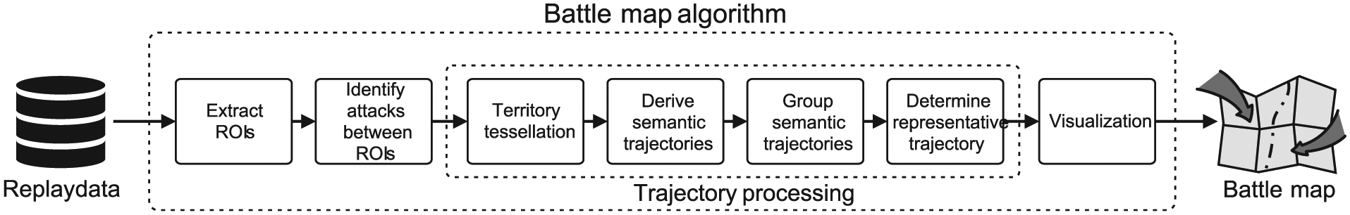
Major steps for creating a battle map from in-game data. First, regions of interest (ROI) are extracted from the input data. Afterwards, fights between ROIs are identified and high-level movements are derived from the individual unit trajectories. Finally, the resulting data are visualized.
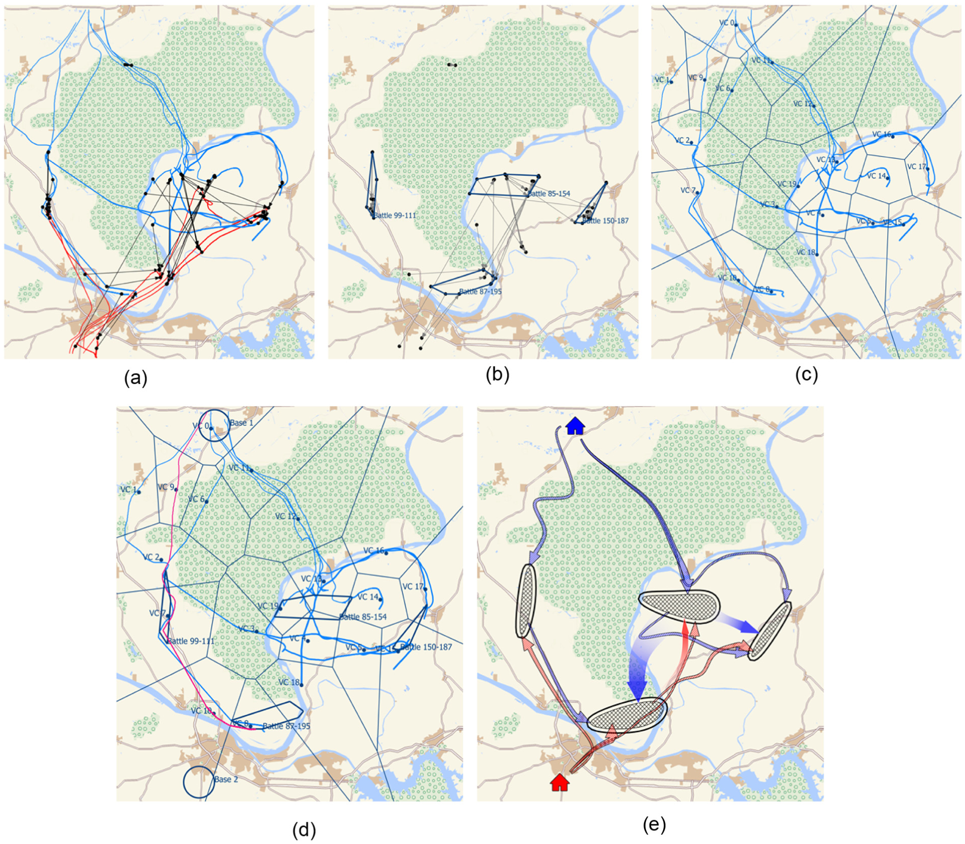
Graphical representation of the result after various steps of the battle map algorithm: (a) input data consisting of unit trajectories, shooting and target positions, and lines of fire, (b) identification of battle regions by spatial and temporal clustering of shooting and target positions, (c) Voronoi tessellation of the area based on trajectory data (calculated separately for each opposing force; in the present case for the blue team), (d) derivation of semantic trajectories based on the ROIs identified in steps (b) and (c) and user-defined ROIs (in this case, base camps), and (e) final map, including battle regions and aggregated movement and attack arrows.
Regions of Interest
The resulting battle map will describe high-level unit movements between certain Regions of Interest (ROIs). Such ROIs can, for example, be base camps, locations of objectives, or places where battles were fought—henceforth referred to as battle regions.
Battle regions can be considered as areas with densely distributed shooting and target positions which occur within short succession of each other. This temporal dimension is an important aspect as battles which take place in the same area but at different points in time should be treated as distinct battles rather than a single entity in order to better reflect the chronology of events. Battle regions are automatically extracted from the input data by employing the DBSCAN clustering algorithm.
41
We have opted for DBSCAN because of its ability to discover clusters of arbitrary shape and varying density (the density of points may differ from battle to battle). In addition, outliers are not assigned to any cluster which is beneficial in our case since occasional encounters distant to dense areas are ignored. Moreover, the number of clusters does not need to be specified in advance. Instead, DBSCAN requires to specify the minimum number of points
The duration of a battle
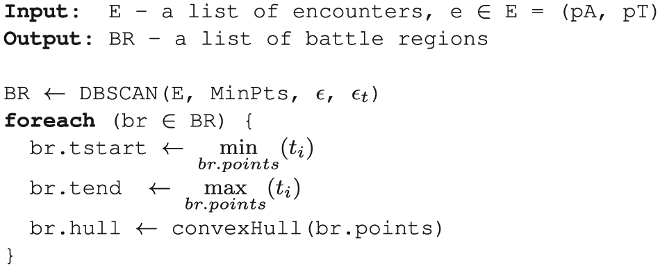
Detection of battle regions (br.points denotes the list of points belonging to the battle region br). Implementation details of the DBSCAN algorithm can be found in Ester et al. 41
Attacks
Once battle regions have been determined, attacks between these regions are identified. Attacks are directed, that is, one region is considered the origin and the other the target of the attack. Thus, at most two attacks between two battle regions

Identification of attacks between battle regions (br indicates the battle region a point belongs to).
Trajectory processing
In this step, individual trajectories are simplified and grouped in order to convey high-level movements between ROIs. For this purpose, the trajectories are first pre-processed by extracting their characteristic points, such as start and end points, pauses, and significant turning points, in order to reduce the computational requirements for the subsequent territory tessellation. Based on the territory tessellation and the ROIs, a semantic trajectory
Territory tessellation
For extracting the characteristic points and territory tessellation (cf. Listing 3), we follow the algorithm described by Andrienko and Andrienko.
20
In short, the algorithm takes as input a set of trajectories, extracts their characteristic points, and clusters these points based on their spatial proximity. The centroids of the clusters are then used as generating points for a Voronoi tessellation. The resulting tessellation thus reflects the spatial distribution of the characteristic points of the original trajectories. The algorithm requires several input parameters which influence the extraction of the characteristic points (namely,
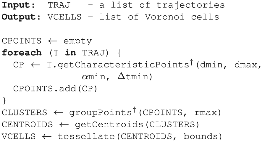
Territory tessellation (bounds denotes the extents of the map,
Semantic trajectories
Next, semantic trajectories
As the final map should show movements between ROIs, the semantic trajectories are then divided into sections, with each section starting and ending at a ROI. For instance, taking our former example,
Derivation of a semantic trajectory from a given trajectory and subsequent decomposition into sections (the function splitIntoSections separates a semantic trajectory into individual sections which all start and end at a ROI by iterating through the list of landmarks).
Grouping of sections
First, sections are partitioned into sets
where

Grouping of sections.
Representative trajectory
As final step, a representative trajectory that describes the overall movement of the individual sections within each group is derived. To this end, we explored two possibilities: one makes use of the medoid and the other is based on computing the central trajectory.
In the former case, the section with the highest average similarity to all other sections within a group is chosen as representative, whereas similarity is again defined by equation (1) (see also Listing 6). With regard to the latter case, first, the parts of the input trajectories covered by the sections of a group—defined by the time a trajectory enters the starting ROI and the time it leaves the target ROI of a section—are determined. Next, the minimum entry time

Derivation of a representative trajectory (medoid approach) for a group of sections.
Visualization
Figure 3(e) shows the final battle map for our ongoing example. To arrive at this representation, a closed Bezier spline is first derived from the convex hull of each battle region. The area enclosed by this curve is cross hatched if close encounters within the area have occurred, that is, when at least one unit within the battle region attacks another unit within the same region. Otherwise (e.g. a group of units of an army is attacked from somewhere else by artillery) the area is left blank. Each battle region is further surrounded by a second slightly inflated and thicker spline curve.
Troop movements are visualized by spline curves derived from the representative trajectories, that is, the centers of the landmarks (either a Voronoi cell or a ROI, see section “Semantic trajectories”) of a representative trajectory are used as control points for a spline curve. Arrow heads are used to indicate the direction of movement. Each spline curve is trimmed at the ends such that it starts at the boundary of the starting ROI and ends at the boundary of the target ROI. Finally, curves are shortened by the length of the arrow heads which, in turn, are bent toward the closest point on the target ROI’s boundary. The direction is further accentuated by the thickness which increases along the curve with the thickness at the base of the arrow head being proportional to the number of involved units. Movement arrows are colored based on the army responsible for the troop transfer.
Attacks are represented by an arrow which is either straight if the attack is unidirectional or slightly bent in case the attack is bidirectional. This way attack arrows between the same two battle regions do not occlude each other. Similar to above, the thickness of the arrow reflects the strength of the attack and the color indicates the army that carried out the attack. In the event that more than one army contributes to an attack then the coloring reflects the share of each army’s contribution. Furthermore, attack arrows are rendered semitransparent such that the map and the movement arrows underneath are still apparent. To reduce occlusions further, arrows are also faded out at their base.
Parameters
The resulting battle map can be influenced by adjusting the control parameters of the various steps outlined above. In the following, these parameters are shortly summarized and explained.
Clustering (
,
,
)
These parameters influence the size and the number of battle regions. Generally speaking, lower numbers for
Characteristic points (
,
,
,
)
These parameters influence how well the simplified trajectories correspond to the original input data. As such these parameters ultimately influence—along with other parameters—the final routing of the movement arrows. For example, simplifying the trajectories too much will remove the subtleties and nuances contained in the original trajectory. A detailed explanation of the effect of the various parameters can be found in Andrienko and Andrienko. 20
Territory tessellation (
)
The parameter
Trajectory aggregation (
)
This parameter controls the number of movement arrows in the final map. The higher the
We should also stress here that providing default parameter values is difficult as the values need to be chosen with respect to the dimension of the game map and should ideally also take the geographical aspects of the map into account (e.g. a narrow urban map may require different parameters compared to a mostly open map). In the reminder of this article, we will assume that all coordinates range from −1 to +1. Figures 4 and 5 illustrate, by way of example, the influence of the trajectory-related parameters and clustering on the generated battle map. Note that

Examples of movement arrows generated by varying the values of the input parameters. Individual unit trajectories are depicted with light blue lines. In each case, the medoid of the groups has been chosen as their representative trajectory: (a) influence of the parameters σ and rmax on the derived movement arrows. A stringent threshold for σ keeps the individual unit trajectories separate (left) while reducing the threshold by half groups the three trajectories together (middle). rmax controls the level of abstraction with smaller values preserving the variations in movement of the representative trajectory and larger radii smoothing out these variations (right). (b) settings for extracting characteristic points (represented by small dots) influence how well the simplified trajectories resemble the original data. Left: fine approximation of the original trajectory. Right: very strong simplification of the input trajectories.

Impact of the clustering parameter
Use case: World of Tanks
In this section, we apply the algorithm to replay data from World of Tanks 15 —a free-to-play massively multiplayer online action game that pits two teams against each other on different maps. Each player controls a single armored vehicle, and once the vehicle gets destroyed, the player is out of the game and cannot re-enter the battle. To win a battle, a team must either destroy all units of the opposing team or capture the enemy base, depending on the game mode.
Methodology
World of Tanks allows the player the record battles and store them in a replay file. Replay files contain information necessary to re-simulate a battle such as unit locations and tanks getting shot or destroyed. However, replay files are recorded from the viewpoint of a specific player. In other words, a replay file only contains the complete movement data from units of the player’s own team. Movement of enemy units is only available while they are within the field of view of the recording player’s team members. This means that in order to reconstruct the full battle, two replay files are necessary, one from a player of each team. To obtain such pairs of replays, we searched the results section of the Wargaming League Europe Bronze Series on the ESL website 45 for matches where replays from both sides were available. All matches which replays are used in the following took place between December 2014 and January 2015. During this period, matches were played in assault mode with two capture circles and each team consisting of seven players. The maximum duration of a match was 7 min. In this mode, one team acts as attacker (henceforth the red army) which has to capture one of the two bases (i.e. capture points) of the defenders or destroy all enemy vehicles in order to win. The defenders (blue army), in turn, have to destroy all attacking units or survive the battle with at least one unit while at the same time protecting their bases from being conquered.
The obtained replays were then decoded and converted to text-based JSON (JavaScript Object Notation) files for further processing using the World of Tanks Replay Parser.
46
Movement data of the individual units can be readily extracted from the JSON files. However, shoot and target locations need to be reconstructed as these locations are not directly stored; rather, the replay contains information which player is doing damage to another player at what time. To determine the shoot and target positions of encounters, we thus use the time-stamp
Results
Figures 6 and 7 show battle maps—along with the original input data—derived from replay data of two battles taking place on the maps: Cliff and Steppes, respectively. In both cases, the centralized path was chosen as the representative trajectory for movement arrows. Capture points (bases) are depicted with a flag while the spawn points of the teams are shown using a cabin icon in the respective color. In case of Cliff, the spawn point of the blue team coincides with the capture point in the north-west corner of the map. Steppes is an open expanse of fields and gentle hills with some rock formations on the boundary of the map offering opportunities for cover and ambush while Cliff features a more mountainous landscape with valleys and rocky hills. Generally, the same settings have been used to generate both maps, but in case of Cliff, the parameter for territory tessellation and the

Red forces win by capturing the enemy base located in the top left corner. Left: input data; right: corresponding battle map (
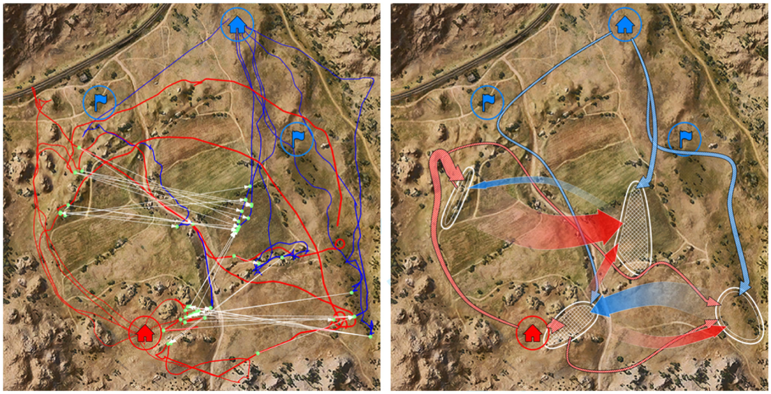
Red forces win by destroying all enemy units. Left: input data; right: corresponding battle map (
In case of Figure 6, the red army followed a more successful strategy, ultimately winning the battle by capturing one of the two bases of the blue team. As evident from the map, the red team has decided to split its forces at its base with the majority of the units moving to the north-east. About half of these units proceeded up the hill located at the eastern side of the map—taking advantage of the elevated position to overlook and attack the blue forces to the north—while the other half took position at the foot of this hill to prevent the enemy team from breaking through. The blue team, however, concentrated all their forces to the east, attacking the tanks of the red army located on the hill and the field below. Meanwhile, a few units of the red team advanced along the valley on the western side of the map to outflank the enemy and capture their base.
Continuing with the second example (Figure 7), the red army has won again but this time by destroying all enemy units. First, the red army moved units to the western flank of the battlefield using the rock formations as cover and firing at the enemy units moving toward the open field in the center of the map. Counterattack by the blue forces proved less efficient—either because the tanks of the red team were more difficult to hit due to the shelter provided by the rocks or because players were less skilled—as conveyed by the much thinner blue attack arrow. Second, the red team has positioned some tanks immediately to the east of its base to defend it against the blue forces. These tanks were heavily under fire from the blue army’s tanks located at the eastern flank while at the same time attacking units located in the battle regions to the east and north. Close combat concentrated on the two battle regions (cross hatched) in the middle of the map.
Figures 8 and 9 show two further examples to illustrate how changes in the parameters influence the resulting battle maps. Figure 8 shows a battle that took place on the game map Himmelsdorf—an urban map largely made up of narrow streets. To account for this confined environment, the left map depicted in Figure 8 uses a small value of 0.1 for
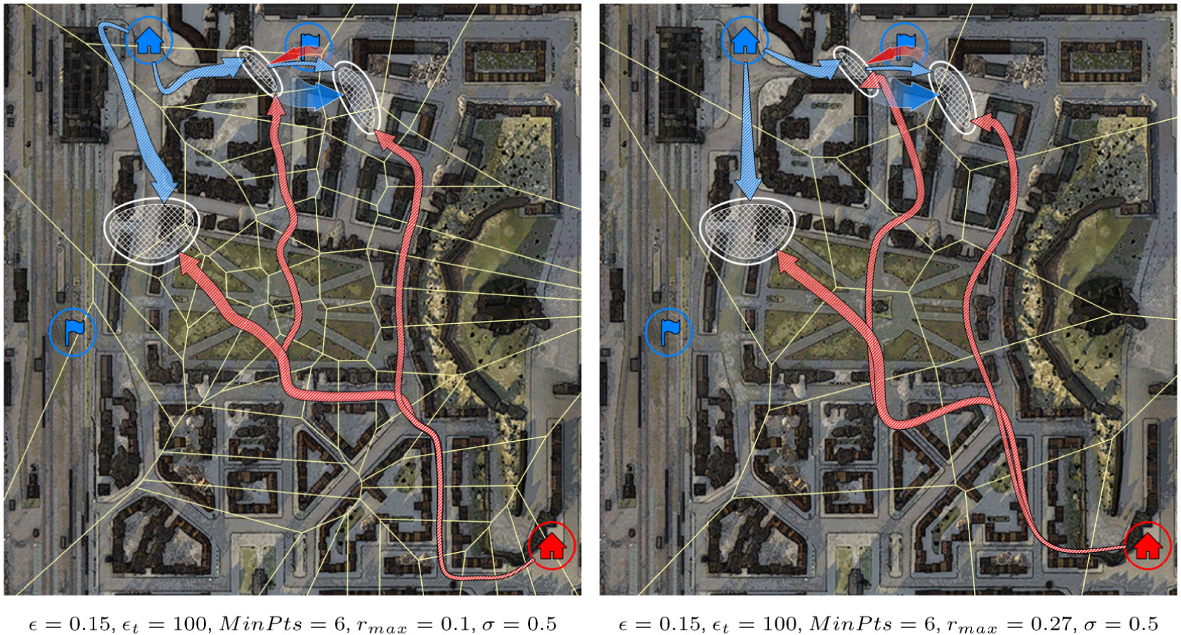
Varying
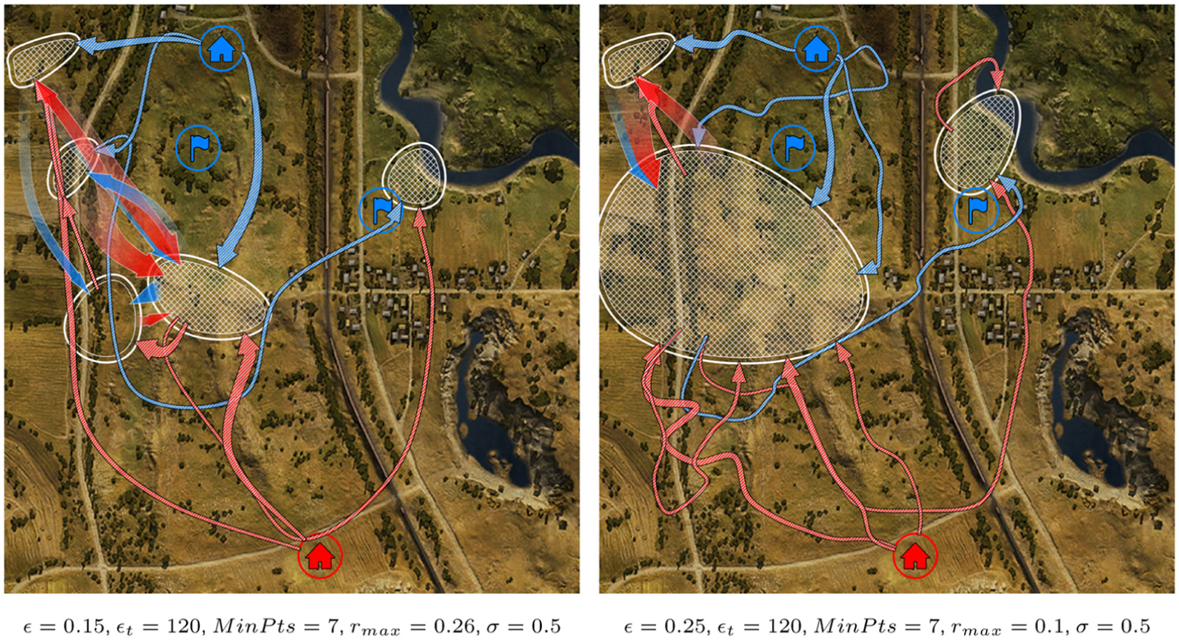
The clustering parameters
The battle depicted in Figure 9 was fought on the map Prohorovka, a map offering large expanses of open but hilly terrain with clusters of trees and little opportunities for cover. As with the Steppes map above, these open spaces allow for more variety and freedom in movement. To smooth out these subtleties, a larger threshold of
Evaluation
To assess the appropriateness of our approach for post hoc battle analysis, we conducted an evaluation with World of Tanks players by means of an online survey. The survey compared three battle visualizations, including the battle map discussed here, the so-called versus view offered by the popular statistics website vBAddict 6 which juxtaposes two maps with each one showing the battle from the perspective of one team, and one-third visualization which merges the two views of the versus visualization and augments it with the lines of fire (akin to the visualization used to visualize the input data in this article, for example, Figure 7, left).
All three visualizations were evaluated, among others, with respect to different cartographic and data visualization design principles such as clarity and esthetics, how well the maps can be interpreted, and for which tasks the visualizations are deemed suitable. For each visualization, three versions (based on different replay files, including the maps shown in Figures 6 and 7) were created yielding a total of nine visualizations of which each participant was shown three (one of each type) in randomized order to control for ordering effects. The results of this evaluation are described in detail elsewhere. 16 Nevertheless, in order to make this article self-contained, we will summarize the most important findings concerning the battle map in the following.
In total, we received 41 complete responses from players aged 15–51 years (
Figure 10 summarizes the ratings (across all three maps) of the battle map with respect to seven different quality measures which were rated by the participants on a 5-point scale anchored by poor (1) and excellent (5). In general, the visualization was rated quite positively with mainly accuracy and ease of extraction being rated lower. The lower ratings in case of the former are, however, not surprising giving that the battle map approach trades accuracy for a concise and high-level view of a battle. In terms of the latter, participants were divided in their ratings with some of them finding it easier to extract information from a battle map than others. However, these mixed ratings are only partly reflected by the data collected to assess how well the visualization is interpreted by the players. For that purpose, each participant had to answer 10 true/false statements which covered different facets of the depicted battle, including questions about troop movements and attacks (to avoid ambiguities in the statements and ease referencing of areas, labels were added to the visualizations). As a consequence, these statements differed from battle map to battle map, yielding a total of 30 questions. For example, concerning troop movements, the survey included statements such as Team 1 moved part of their units to area B and then continued to area C with the same number of units or Team 1 split its forces at their base with the larger fraction going to area A. Examples of attack-related statements are as follows: Attack rate from area A to C was larger than from C to A; A battle between units of different teams took place within area A; and Team 2 attacked units in area A from areas B and C.

Boxplot—median, interquartile range, minimum, and maximum (whiskers)—summarizing the ratings (1 = poor, 5 = excellent) with respect to seven different criteria.
On average, statements were answered correctly by 84.3% of the respondents. Participants mostly struggled with statements concerned about troop movements when movement arrows of the same color were overlapping each other like it is, for example, the case for the red arrows in Figure 6 (right). In such cases, the mean correctness ranged between 40.0% and 64.3%.
As part of the online questionnaire, participants were also asked for which types of questions they believe the battle map is most suitable. A qualitative content analysis (cf. Schreier 47 ) identified five major categories of questions for which the battle map was considered useful, namely, questions concerning:
Areas of interest such as zones of conflict, areas where troops gather, or choke points (18 statements)
Map strategies and tactics (12 statements)
Team movements (11 statements)
A quick overview of the flow of battle (8 statements) and, to a lesser degree, also for questions about
Combat (5 statements)
However, participants found the visualization to be particularly ill suited for questions dealing with the movement and positioning of individual units as well as for understanding aspects of reconnaissance such as where enemy units were spotted. In summary, we can state that the battle map proved to be suitable for gaining a general understanding of a battle, that is, high-level information about areas of interest and troop movements. The good readability and the general overview of a battle were also the major reasons for some participants to prefer the battle map over the other two investigated visualizations. For others, however, the lack of detail was the main reason for ranking the battle map lower in terms of personal preference.
In addition, to the results summarized above and reported previously,
16
we asked players (
However, when asked about if the battle maps contain any unnecessary information, almost all participants (92.7%) agreed that none of the elements displayed is superfluous.
Discussion
When interpreting the results of the player questionnaire presented above, it should be kept in mind that all the respondents were rather experienced World of Tanks players and as such are likely to have certain expectations on what information should be represented in a battle summary. This may also explain the comparatively low rating of accuracy as experienced players may be more interested in more detailed information (e.g. spotting of enemy units, exact locations of kills) than, for example, casual players. However, we should point out that our evaluation 16 did not show any correlation between the accuracy rating and the number of collected experience points nor with the number of battles fought, though this might result from the our skewed sample toward highly experienced player. In future work, it may thus be worthwhile to explore differences between novices and experts in greater detail.
Further work will also focus on ways to include the additional information asked for by the participants (e.g. information about troop strengths, kill locations, details about units, and battle outcomes) into the battle map visualization. For example, the strength of forces could be conveyed by adding numerical labels to movement arrows and the outcomes of battle sites could be indicated by coloring the hull enclosing a battle region with the winning team’s color. However, a fundamental challenge in map making is to avoid information overload while at the same time ensuring clarity and readability. At this point, we should also emphasize that the goal of this work was to produce maps which provide all the important information regarding a battle at a single glance. A natural progression of this work would thus be to explore ways of including more detailed information by offering possibilities for interaction. For instance, details regarding the types of unit troops are composed of or about the particulars of a battle (e.g. types and number of units lost) could be displayed on demand with tooltips while information about the exact locations of kills and lines of fire could be displayed by allowing users to zoom into battle regions.
Apart from this, one of our next steps will also be to explore ways to reduce the visual complexity further. As our evaluation has shown, players had difficulties to correctly trace the movement of troops in case the arrows (partly) occluded each other. One possible solution could be to—instead of using individual arrows—merge arrows together as long as they follow the same route. For example, the two red movement arrows running along the eastern border of the map in Figure 6 (right) could be merged into a single arrow which splits into two distinct branches after the valley. This would reduce overlappings of arrows and perhaps also convey troop strengths more clearly.
In this article, we used data from World of Tanks to demonstrate our approach because (a) its theme and gameplay make it well suited for the technique presented here and (b) it is one of the few games which currently exposes all the necessary data. However, it should be emphasized that the algorithm is general enough to be applied to other games with similar gameplay mechanics or where more than two teams compete against each other as well—as long as the game provides time-stamped data on the trajectories of the units as well as about the shooting and target locations.
One drawback of the datasets we had available is the relatively small number of players on which they are based. However, most online multiplayer games similar to World of Tanks limit the number of concurrent players per battle to a few tens for performance or gameplay reasons. Battle maps for strategy games may be computationally more expensive to compute because such games may involve hundreds of units per player. However, given the computational complexity of the various steps, we expect the algorithm to also scale well to larger datasets. Extracting the battle regions with DBSCAN has an average runtime complexity of
With regard to the representative trajectory, we found that both the medoid- and centroid-based approaches produce visually similar results in case a high similarity threshold is used to group the trajectory sections and if the territory is finely tessellated. However, if the sections in a group become more dissimilar, the average central trajectory may deviate too much from the routes actually taken (due to averaging the locations) and may thus lead to false impressions. In such cases, we found the medoid to be more suitable because it corresponds to an actual route taken by a unit. However, this issue should be explored in more detail in the future.
Conclusion
In this article, we described an algorithm for generating battle maps based on in-game data. Several parameters can be adjusted to control the level-of-detail desired in the final map. As proof-of-concept we used the algorithm to produce battle maps based on replay data from World of Tanks. However, the algorithm is not restricted to this specific game but can be applied to other games as well, provided that the game records unit trajectories as well as shooting and target locations. Feedback was generally positive with players highlighting especially the good readability of the battle maps and the concise general overview they offer. However, future work may concentrate on finding ways to include more detailed information to further improve the utility of the approach. Moreover, while player feedback showed the appropriateness of the approach for retrospective analysis of battles, more detailed long-term studies will be required to better understand how effective the visualization is for skill-building, that is, does analyzing battle maps result in better in-game performance.
Footnotes
Acknowledgements
The author thanks all the participants who took part in the evaluation for their valuable contributions.
Funding
The author(s) received no financial support for the research, authorship, and/or publication of this article.