



Abstract
This paper describes in detail the process for predicting, from first principles, the rotor–stator interaction tone levels for two realistic model-scale fans that are representative of high bypass ratio and ultrahigh bypass ratio turbofans. The prediction scheme relies on a suite of three-dimensional computational tools that include Reynolds Averaged Navier–Stokes aerodynamic models and linearized inviscid aeroacoustic models. The goal of the study was to assess the accuracy of tone-level predictions for realistic fans operating under realistic conditions. The predictions were carried out over a wide range of operating conditions that include, but were not limited to the approach, cutback, and sideline conditions for each of the two fans. The in-duct and external tonal sound fields were computed at a representative blade passing frequency harmonic tone. The predicted tone sound pressure level and sound power level have been compared with the measurements acquired at a NASA anechoic wind tunnel. The data–theory comparisons are primarily focused on the exhaust tone levels due to lack of validated models for predicting the three-dimensional tone acoustic transmission through a rotor. The data–theory comparisons show that it is possible to make accurate predictions of the exhaust rotor–stator interaction tone power levels starting with the geometry of the fan stage. Specifically, the results demonstrate that the exhaust rotor–stator interaction tone power levels can be predicted to within
Introduction
Fan tones are a ubiquitous feature of turbofan engine noise spectra. Their presence is an inevitable consequence of the aerodynamic interaction between the fan and outlet guide vanes. Specifically, fan tones are generated (at the harmonics of the blade passing frequency (BPF)) as a result of the impingement of the periodic component of the fan rotor wakes on the bypass duct outlet guide vanes (OGV). For that reason, this source is often referred to as the rotor–stator (R/S) interaction tone noise. The interaction tones are a source of annoyance requiring careful consideration when choosing the blade/vane count ratio of the fan stage in order to minimize their strength or tailor their modal content to increase the efficacy of the nacelle liners. Consequently, it is not surprising that, over the years, significant research has been devoted to the development of tools for the prediction of R/S interaction tone levels for realistic fan stages. These efforts have led to a number of theoretical models that range from purely analytical to purely numerical in nature.
The initial efforts were focused on analytical models in which the three-dimensional fan stage geometry and the aerodynamic interaction between the blade rows are greatly simplified in order to make the mathematics tractable.1–7 Experience indicates that while such models provide closed-form expressions that loosely connect the interaction tone spectrum to some important geometric features and aerodynamic parameters of the fan stage, they do so at the expense of fidelity and accuracy. As a result, a few basic trends can typically be investigated using analytical models, but absolute spectral levels and nuances of the tone spectrum cannot.
The application of acoustic analogy, in which the aerodynamic and acoustic aspects of the problem are conveniently separated, provides some improvement in fidelity and accuracy. That is because CFD-based description of the rotor wakes or the fluctuating loading on the OGV can be used as input to the acoustic model. Of course, the acoustic model typically remains idealized in its description of the flow and/or geometry of the outlet guide vanes.8,9 These models may provide more reasonable estimates of the fan tone characteristics, but still fail to yield reliably accurate absolute level predictions on a consistent basis.
With the advent and rapid development of the three-dimensional computational aeroacoustic approaches, there has been a marked improvement in the state-of-the-art for the prediction of R/S interaction tone levels. In these approaches, the complexity of the fan stage geometry and its flowfield is retained, and the resulting governing equations are solved numerically. Depending on the level of fidelity of the flowfield that is retained in the governing equations, these methods run the gamut from the linearized (viscous/inviscid) methods to the fully nonlinear methods in both the frequency and time domains.10–15 The linearized methods rely on the CFD-based description of the fan wakes, while the nonlinear viscous approaches solve for the complete unsteady flowfield from which acoustic content can be extracted. Published literature suggests that the prediction of fan tone levels using modern computational tools requires relatively modest computational resources that are well within the reach of aircraft engine manufacturers. In fact, it may well be that over the next few years, the computational tools will supplant the traditional analytical/semi-analytical models for predicting and optimizing fan tone spectra.
This paper summarizes a study that was undertaken to explore in detail the accuracy of representative three-dimensional computational aerodynamic and aeroacoustic models for the prediction of the R/S interaction tone levels for realistic fans. a The focus here is on the fan aft-radiated (i.e., exhaust) tone noise as there are no validated models for calculating the three-dimensional transmission of acoustic waves through a rotor (especially in the presence of swirling flow), which is a necessary ingredient for the accurate prediction of the fan inlet tone levels. The study focuses on the prediction of the second harmonic of the BPF tone for two 22″ (0.56 m) diameter model-scale fans for which extensive aerodynamic and acoustic data have been acquired in NASA’s 9 ft × 15 ft (2.74 m × 4.57 m) low-speed acoustic wind tunnel. The viscous fan wakes and other aerodynamic input needed for the acoustic predictions have been extracted from a series of Reynolds Averaged Navier–Stokes (RANS) aerodynamic simulations of the two fan stages. In-duct sound pressure level (SPL), sound power level (PWL), and sideline directivity of SPL have been predicted using linearized inviscid models. The predictions (both aerodynamic and acoustic) have been compared with the measured data obtained in the wind tunnel. In the next few sections, the benchmark model fans, the experimental setup and data, and the prediction methodologies used in this study are described in detail. These sections are followed by the presentation and discussion of the acoustic results, and the paper is concluded with a summary section describing the main conclusions drawn from this study and recommendations for future improvements.
Benchmark fans and experimental data
Model stage fan design parameters.
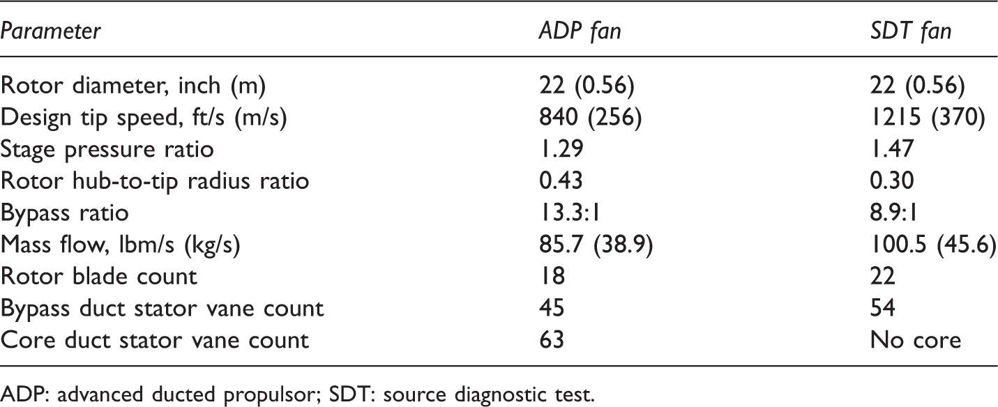
ADP: advanced ducted propulsor; SDT: source diagnostic test.
Fan rotational speeds investigated in this study.
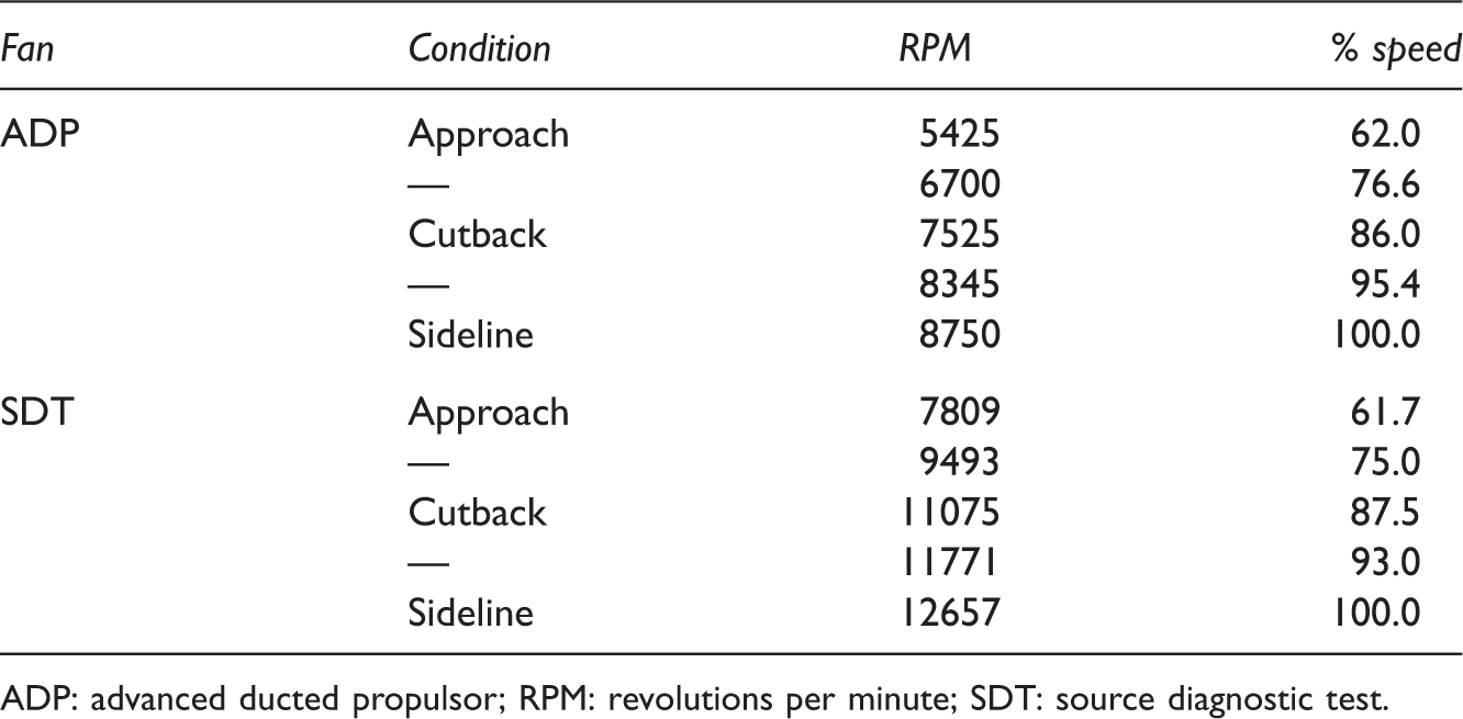
ADP: advanced ducted propulsor; RPM: revolutions per minute; SDT: source diagnostic test.
Mode SPLs and PWLs (underlined) for ADP at 2BPF as predicted by LINFLUX.

ADP: advanced ducted propulsor; BPF: blade passing frequency; PWL: sound power level; RPM: revolutions per minute; SPL: sound pressure level.
Mode SPLs and PWLs (underlined) for SDT at 2BPF as predicted by LINFLUX.
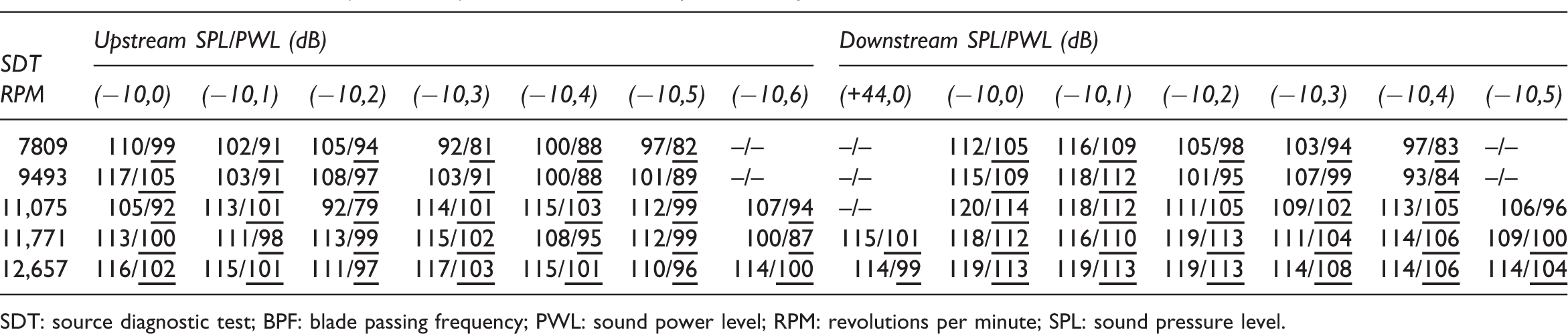
SDT: source diagnostic test; BPF: blade passing frequency; PWL: sound power level; RPM: revolutions per minute; SPL: sound pressure level.
Comparisons of predicted (LINFLUX) and measured 2BPF PWL.

ADP: advanced ducted propulsor; BPF: blade passing frequency; PWL: sound power level; RPM: revolutions per minute; SDT: source diagnostic test.
Mode SPLs for ADP at 2BPF: LINFLUX versus analytical model (underlined).

ADP: advanced ducted propulsor; BPF: blade passing frequency; PWL: sound power level; RPM: revolutions per minute; SPL: sound pressure level.
Mode PWLs for ADP at 2BPF: LINFLUX versus analytical model (underlined).
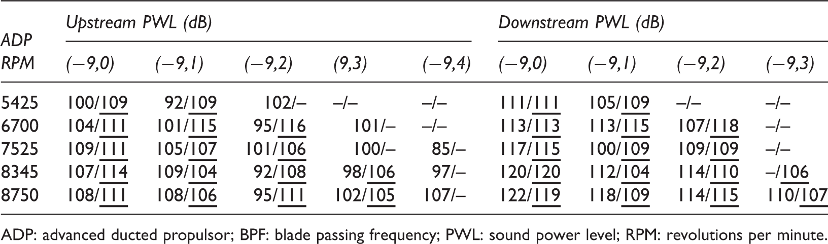
ADP: advanced ducted propulsor; BPF: blade passing frequency; PWL: sound power level; RPM: revolutions per minute.
Mode SPLs for SDT at 2BPF: LINFLUX versus analytical model (underlined).
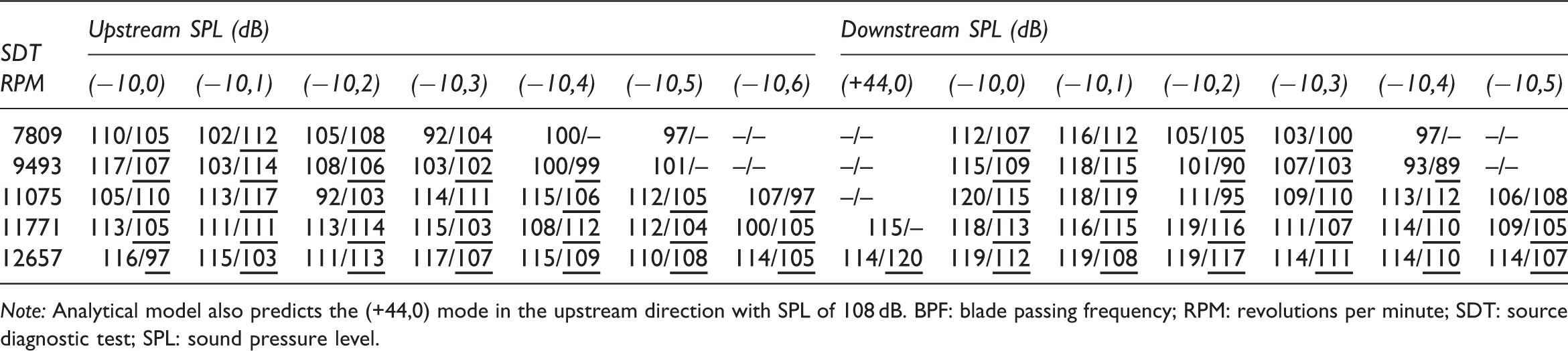
Note: Analytical model also predicts the (+44,0) mode in the upstream direction with SPL of 108 dB. BPF: blade passing frequency; RPM: revolutions per minute; SDT: source diagnostic test; SPL: sound pressure level.
Mode PWLs for SDT at 2BPF: LINFLUX versus analytical model (underlined).
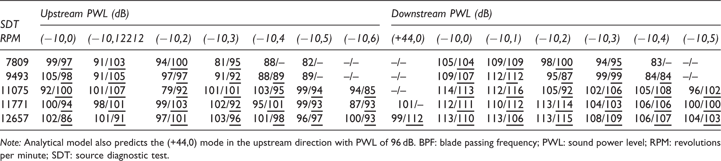
Note: Analytical model also predicts the (+44,0) mode in the upstream direction with PWL of 96 dB. BPF: blade passing frequency; PWL: sound power level; RPM: revolutions per minute; SDT: source diagnostic test.
The 9 ft × 15 ft is a continuous-flow, anechoic wind tunnel capable of simulating flight speeds of up to Mach 0.23. The test section is acoustically treated and is anechoic down to 250 Hz, 17 a limit which is well below all of the tone frequencies considered in this study. Finally, all fan acoustic data used in this study were acquired at the tunnel Mach number of 0.1.
Photographs of the two fan stages are shown in Figure 1 as are the three-dimensional cutaways of their internal geometry. ADP has a passive core with an inlet guide vane, but SDT has no core duct. There are no bifurcations or pylons in the aft-fan ducts, so both fans are ideally suited for studying the R/S interaction tones. Aerodynamic and acoustic data for the two fans had been acquired18–29 at different times as part of the past NASA acoustic test campaigns funded by various NASA aeronautics research projects.
Top row: The 22″ model scale ADP and SDT fan stages installed in the NASA 9 ft × 15-ft Low-Speed Acoustic Wind Tunnel. Bottom row: Cross-sectional sketches of the two fans. The ADP fan has 18 fan blades and 45 bypass OGVs. The SDT fan has 22 blades and 54 bypass OGVs. ADP: advanced ducted propulsor; OGV: outlet guide vane; SDT: source diagnostic test.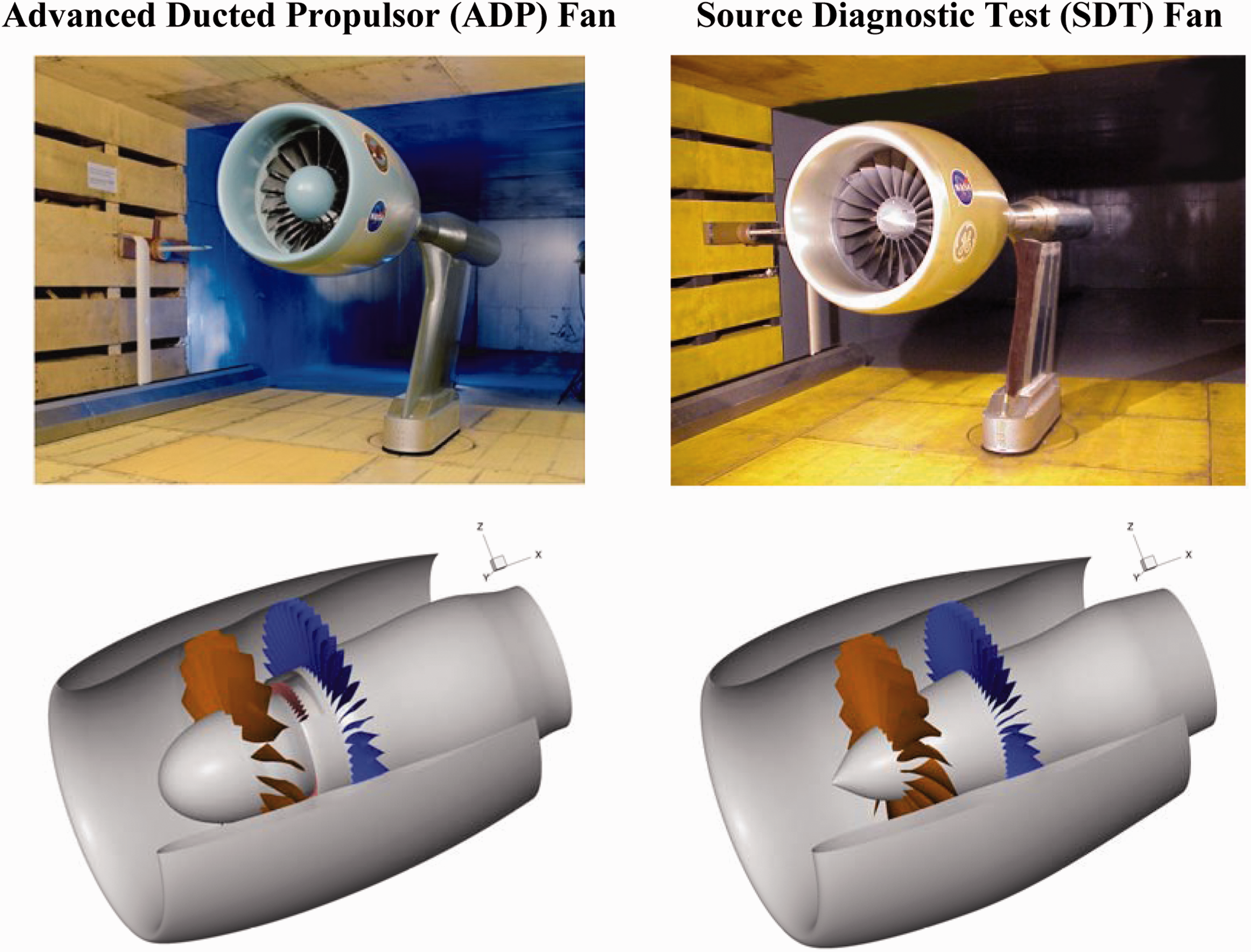
The acoustic test layout is depicted in Figure 2, which shows the plan view of the 9 ft × 15 ft acoustic wind tunnel with the fan stage installed. The acoustic data were acquired using a quarter-inch (0.64 cm) microphone that moves on a sideline track that is parallel to and displaced horizontally 89.3″ (2.27 m) from the vertical symmetry plane of the fan. In other words, the traversing track is slightly more than four rotor tip diameters away from the fan axis. The traversing microphone itself is located at the same height from the tunnel floor as the fan rotational axis. Acoustic pressure data were acquired at 48 positions (i.e., sideline angles) along the traverse track at approximately 2.5° intervals. The sideline angle θ is defined such that the upstream infinity is at 0° and the downstream infinity at 180°. The range of sideline angles subtended by the track is from 27° to 135°. Three fixed microphones are also typically used to extend the aft angular coverage, as shown in Figure 2. They provide data at 140°, 150°, and 160°. The microphone data are corrected for the frequency-dependent atmospheric absorption of the acoustic signals as they propagate from the fan to the microphone. The corrected microphone data are converted to SPL using the reference pressure of 2 × 10⁻⁵ Pa. Sideline SPLs are also projected onto a circular arc and integrated over the angular range of 27° to 160° to calculate the acoustic PWL using the reference power level of 10−12 W. The contribution of SPL outside this angular range is ignored. The projection of SPL data from the sideline track to the circular arc is carried out assuming that the sideline data are in the farfield and by applying the spherical spreading rule.
Plan view of the NASA 9 ft × 15 ft wind tunnel test section showing the model fan rig, traversing microphone, and fixed microphones. Dimensions are in inches (meters).
The acoustic data were acquired both with and without a barrier wall in order to isolate inlet- and exhaust-radiated tone level contributions. The barrier wall, which is offset 6″ (15 cm) from the nacelle, extends vertically from the floor to the ceiling of the tunnel and axially from the nacelle inlet plane to a station well downstream of the fan rig. As indicated in Figure 2, when the barrier wall is in place, the microphones are shielded from the fan exhaust tones and only inlet-radiated tones are measured. Without the wall, the microphones measure contributions from both the inlet and exhaust. The difference between the two provides an estimate of the exhaust-radiated tone levels. With the barrier wall in place, the three fixed microphones are removed, and only the 48 stops on the track are used for measurements.
Acoustic prediction methodology
The aeroacoustic prediction methodology used in this study is based on an unsteady three-dimensional linearized inviscid analysis of the R/S interaction.30–32 The mathematical formalism, which is expressed as a problem in the frequency domain, is fairly general and can be used for predicting the aeroacoustic as well as the aeroelastic response of a blade row to flow perturbations in axial flow turbomachinery.
The theoretical model is embodied in a code called LINFLUX, which requires a three-dimensional steady, nonlinear, inviscid base flow for the OGV. The base flow is most conveniently generated by a companion code called TURBO, 33 which, like LINFLUX, is a finite-volume code and uses the same grid topology and, in fact, the same computational domain and grid as LINFLUX. With the base flow specified, LINFLUX computes the acoustic response of the OGV to incident vortical perturbations (i.e., the wakes of the rotor) riding on the base flow at a given BPF harmonic. LINFLUX calculates the acoustic response to the incident vortical perturbations by matching the three-dimensional perturbation solution in the computational domain to the modal descriptions of unsteady perturbations for idealized base flows that are assumed to exist upstream and downstream of the LINFLUX computational domain. These flows are assumed to depend only on the radial coordinate and include swirl and shear as appropriate to the OGV inflow and outflow boundaries. Within these idealized base flows, the perturbation field is approximated as a combination of acoustically dominated modes and convective vortical modes. The modal descriptions are numerically computed from the eigenvalue problems for these idealized base flows subject to the appropriate duct wall boundary conditions. b The main output of LINFLUX is the first-order perturbations in density, momenta, and total energy. In addition, LINFLUX also computes the outgoing acoustic field at the domain’s inflow and outflow planes in terms of a finite number of circumferential and radial acoustic modes. Some of these modes are propagating for which LINFLUX computes SPL and PWL. The rest are a few of the least damped evanescent acoustic modes. A description of how LINFLUX computes the acoustic power level will be given in the section titled Acoustic predictions.
For a fully predictive approach to the computation of R/S interaction tone levels, the incident rotor wake perturbations that drive the acoustic response are typically extracted from suitable viscous simulations of the fan stage. For the purposes of this study, the rotor wakes were extracted from a set of aerodynamic simulations for the ADP and SDT fan stages that were computed under contract to NASA and used for a series of aeroacoustic studies.36,37 These simulations, which model the flowfields both inside and outside of the nacelle, were carried out at the five fan rpm listed in Table 2 to match the experimental conditions in the wind tunnel for which the aerodynamic and acoustic data had been acquired.
The aerodynamic simulations were generated using an axisymmetric viscous flow solver called AVCS 38 coupled to a three-dimensional viscous turbomachinery flow solver called TSWIFT. 38 These codes are based on similar algorithms, have multi-block capability, and solve the RANS-based flow equations on body-fitted grids using an explicit finite difference scheme. The simulations included the entire fan system, therefore, only the rpm and fan stage exit static pressure ratio were adjusted in order to set the fan operating point and ensure that the predicted mass flow rates matched the measurement values accurately. The codes output the distributions of the density, momenta, and total energy variables as well as such turbulence parameters as the eddy viscosity, turbulence kinetic energy, specific dissipation rate, and so on.
A meridional plane view of the aerodynamic computational domain is shown in the top portion of Figure 3 using the ADP fan stage results as an example. The figure shows the axisymmetric Mach number distribution in the computational domain with a fan blade, an OGV stator, and a core inlet guide vane (IGV) stator superimposed on the domain to show their relative positions. The actual domain extends far beyond the stage in all directions, but in the interest of showing the details of the fan stage clearly, this view is zoomed in. The external Mach number in all simulation cases was set to 0.1, which was the tunnel speed at which all of the aerodynamic and acoustic data had been obtained. It should be noted that the core in the ADP fan stage model is passive. In the case of ADP, the static pressure downstream of the IGV was adjusted to ensure the proper mass flow split between the bypass and core ducts was achieved. Because SDT does not have a simulated core, no such adjustment was necessary.
Top: Domain for the aerodynamic simulations includes both the internal and external flowpaths. Mach Number distribution for the advanced ducted propulsor fan stage at 8750 r/min is shown as an example. Aerodynamic calculations are multi-block and RANS based. Bottom: Domain for the acoustic calculations includes the region straddling the OGV. The acoustic calculations are linearized Euler based. OGV: outlet guide vane; RANS: Reynolds Averaged Navier–Stokes.
The bottom portion of Figure 3 shows a further zoomed-in view of the internal flowpath of the ADP fan stage, where the extent of the computational domain used in LINFLUX is indicated by the two solid black lines. The domain straddles the OGV and extends one axial chord upstream of its leading edge and one axial chord downstream of its trailing edge. This ensures that there is sufficient distance away from the OGV for a proper acoustic mode structure to form while also avoiding excessive duct area changes. Two other locations are also indicated in the figure by the dashed black lines. The one marked as the “Axial Station 1” is approximately 4″ (10 cm) downstream of the stacking axes of two fans and is the location where two-component (i.e., axial and tangential) mean flow velocity data were acquired for both fans at the approach, cutback, and sideline operating conditions using the laser Doppler velocitmetry (LDV) technique in the wind tunnel.
c
The axial and tangential mean velocity components (namely,
A typical comparison is shown in Figure 4 for both fans at the sideline operating condition. In the top row, the results for the ADP fan are shown and in the bottom row those for the SDT fan. The left hand side of the figure shows the LDV-measured axial velocity distributions and the right hand side shows the predicted axial velocity distributions. For each fan, the measured and predicted velocity contours are plotted on the same scale and over the same range. The LDV measurements did not extend to the duct wall regions in order to avoid laser beam reflections from the duct walls, but the simulations extend all the way to the duct walls. All of the gross features of the flowfield are captured quite well in the simulations and the levels are comparable too. For a more quantitative comparison, pitchwise profiles are extracted from the contour plots at 25%, 50%, and 75% spanwise locations, respectively, and are compared in Figure 5. The pitchwise coordinate (expressed in degrees) is shifted so that the wake profiles are centered on the 0° location. Typically for these simulations, the RANS-based wakes are deeper (i.e., less diffused) than the measured ones with a maximum discrepancy of 10%. The maximum discrepancy in the free stream velocity in the passage is less than 5%, though in most cases the difference is significantly smaller. As the acoustic field is linearly related to the incident wake perturbations, these discrepancies ( Contours of axial velocity for the advanced ducted propulsor fan (top row) and source diagnostic test fan (bottom row) at the Axial Station 1 (i.e., 4″ downstream of the rotors stacking axes). Laser Doppler velocitmetry data are shown in the left column and the Reynolds Averaged Navier–Stokes prediction in the right column. Comparisons are shown for the sideline tip speed for both fans. Comparisons of laser Doppler velocitmetry and Reynolds Averaged Navier–Stokes pitchwise axial velocity profiles at three spanwise locations at Axial Station 1 for advanced ducted propulsor on the left and source diagnostic test on the right.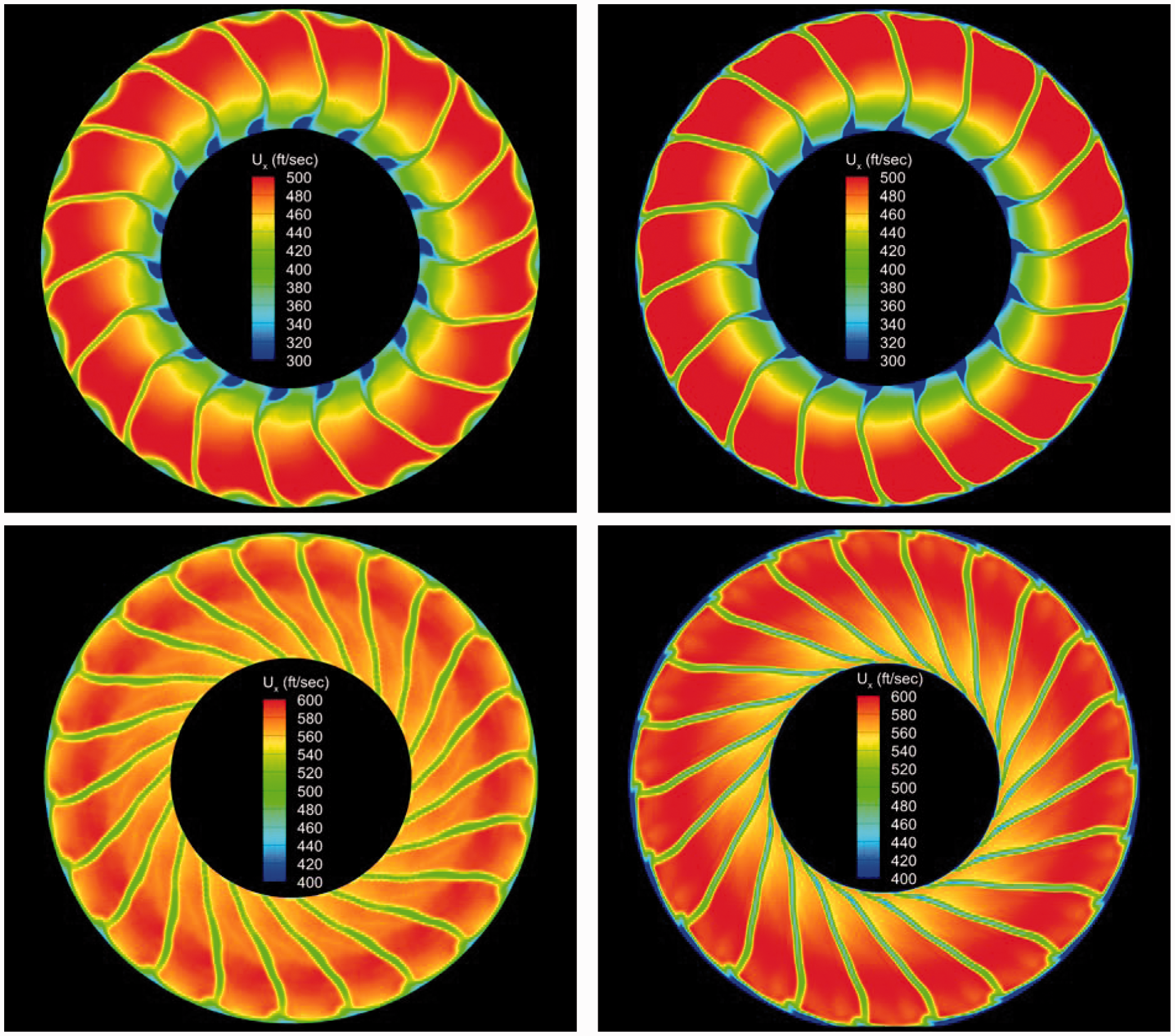
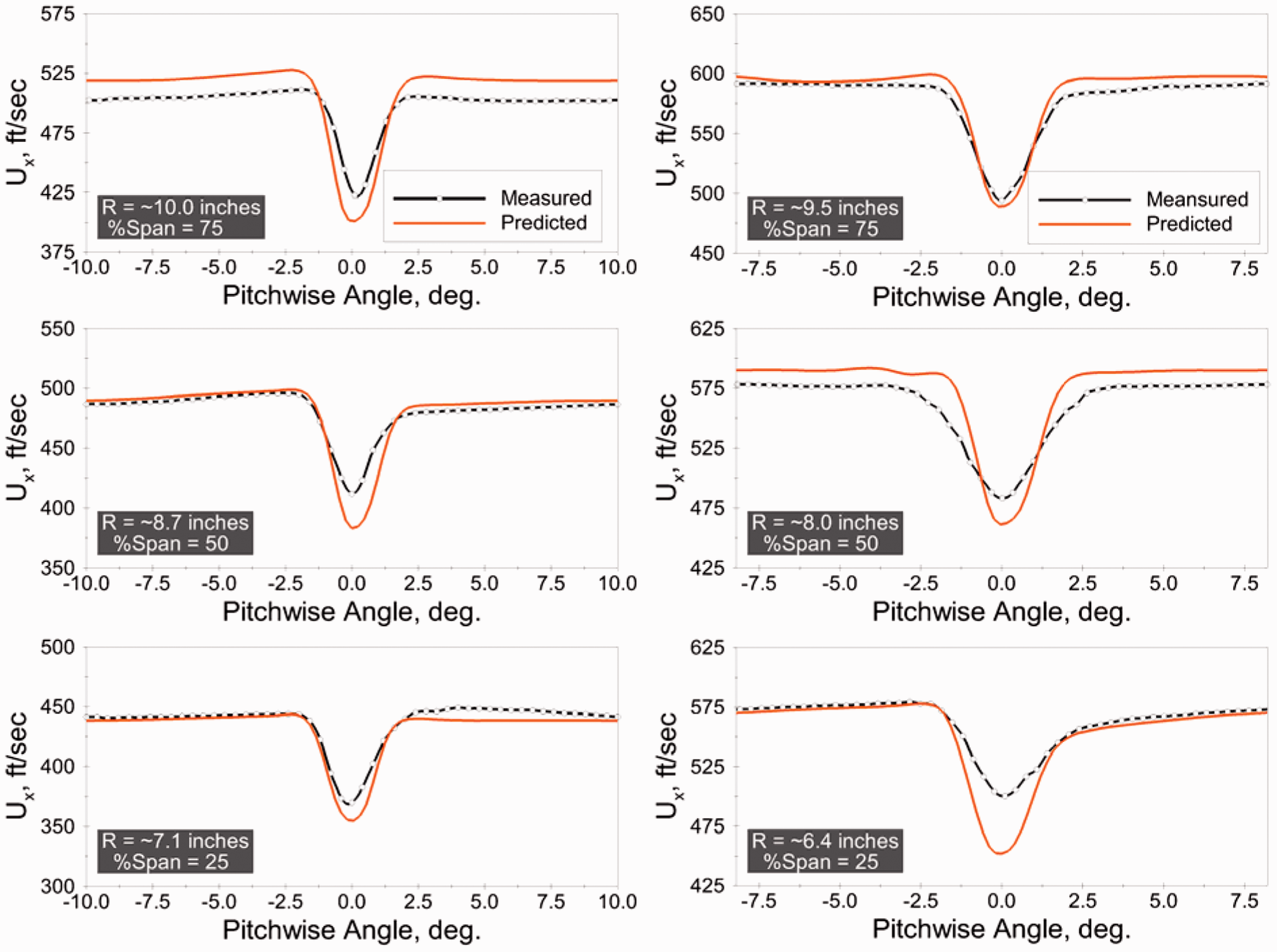
Finally, it should be noted, as the results in Figures 4 and 5 suggest, the level of data–theory agreement for the rotor wakes is comparable regardless of whether the tip relative speed is subsonic (as it is for all the ADP operating conditions) or supersonic (as it is for some of the SDT operating conditions). In other words, the quality of the predicted rotor wakes used in this study is not adversely affected by the presence of the rotor-locked shock field.
It might be natural to think that for the purposes of the acoustic calculations, the fan wake profiles should be extracted from the RANS solutions at the axial location of the inflow plane to the LINFLUX computational domain (see Figure 3). However, since LINFLUX is inviscid it cannot properly model the viscous evolution of the rotor wake (i.e., its viscous diffusion) as the wake convects downstream before reaching the OGV. e To circumvent this difficulty, the wake profiles are extracted at a station close to the OGV leading edge (i.e., Axial Station 2 depicted in Figure 3) and used as input to LINFLUX. As such, the wake profiles will have the correct viscous evolution (i.e., proper decay), at least according to the RANS paradigm. However, they will also have excessive tangential lean. f As such, the wake profiles extracted at the OGV leading edge must be shifted (axially and tangentially) to ensure that the rotor wakes have the lean associated with the LINFLUX inflow plane’s axial location. Failing to do so would effectively make the lean of the wakes more pronounced when they are convected by LINFLUX to the OGV leading edge thus introducing errors in the predicted tone levels. It is known that tone levels depend sensitively on the spanwise lean of the wake relative to the OGV leading edge. 41 The axial and tangential shifts from the OGV leading edge to the inflow plane are accomplished in an approximate manner in that the input wake velocity perturbations are assumed to be functions of the axial and tangential coordinates but depend only parametrically on the radial coordinate. Furthermore, these perturbations are assumed to have no associated pressure or density fluctuations. As such, input wake velocity perturbations satisfy the conservations laws for mass, axial and tangential momenta, and energy, but do not conserve the radial momentum.
The rotor wake input to the LINFLUX code is supplied in terms of the pitchwise Fourier series of the wake profiles at a suitable number of radial stations. The complex-valued amplitudes are the coefficients in the Fourier decomposition of the wake profiles in terms of the rotor BPF harmonics. The input for the companion TURBO code, which must be run first, requires the pitchwise-averaged profiles of the total pressure, total temperature, and swirl angle as a function of radius at the inflow plane. Both aerodynamic input sets have been extracted from the RANS simulations discussed earlier. As an example, Figure 6 shows a collage of these profiles for the ADP fan at 8750 r/min.
g
The wake harmonic contents shown in this figure are for the 2BPF component of the wake.
Typical spanwise profiles of the flow parameters needed as input for the TURBO and LINFLUX calculations. The profiles shown are for the advanced ducted propulsor fan operating at 8750 r/min. The wake harmonic profiles are for 2BPF. BPF: blade passing frequency.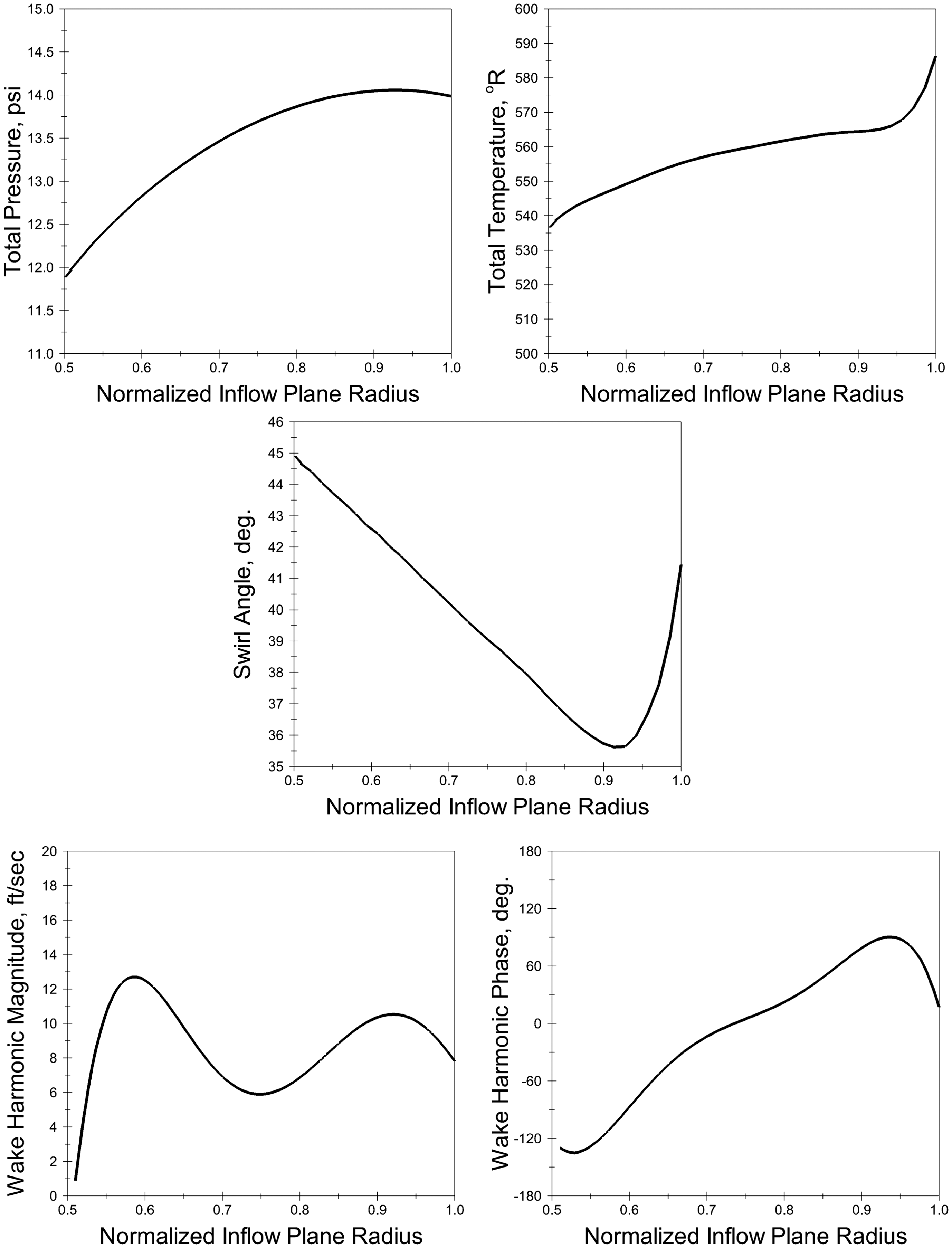
This input information is supplied at the inflow plane of the computational domains for the TURBO and LINFLUX simulations. As mentioned earlier, TURBO and LINFLUX use the same computational domain. The domain, shown in Figure 7, is a single three-dimensional grid block spanning one-vane passage between the suction side of one vane and the pressure side of the adjacent vane (see the left side of the figure). It should be noted that because both TURBO and LINFLUX are inviscid codes, the OGV’s round trailing edge was modified and made sharp in order to avoid flow recirculation downstream of the trailing edge. The modification smoothly extended the airfoil sections by about 6%.
The computational domain used for the TURBO and LINFLUX computations is highlighted on the left. It consists of a single passage between the suction side of one vane and the pressure side of the adjacent vane. Sample grid layers extracted from the domain at the hub, midspan, and tip are shown on the right.
A grid generator program called TIGER
42
was used to create the sheared H-grids topology needed for the TURBO/LINFLUX calculations. The axial × circumferential × radial dimensions of the two grids generated for the ADP and SDT acoustic simulations are 181 × 43 × 49 and 181 × 37 × 51, respectively. The choice of the grid density was guided by experience and the criterion to have an average of 40 grid points per wavelength of the target frequency in the direction of wave propagation (i.e., in the
All TURBO simulations used in this study were carried out up to a maximum of 40,000 iterations in order to ensure that all of the mean flow variables had fully converged. This resulted in the root mean square error being reduced by at least four orders of magnitude. Examination of the results at earlier iteration counts (i.e., 10,000, 20,000, and 30,000) indicates that in most (but not all) cases, the mean flow solution had stabilized after 20,000 iterations and did not require additional iterations. Comparisons of the global variables (e.g., mass flow) and local variables (e.g., pressure and velocity distributions) as computed by TURBO with the corresponding ones from the RANS simulations indicate that in the inviscid regions the agreement is very good and consistent with the expectations. This provided confidence in the inviscid mean flow solutions.
All of the LINFLUX simulations were run 5000 iterations at which point the root mean square error was reduced by six orders of magnitude or more. In fact, in most cases the error had been reduced to that level after about 4000 iterations. It should be noted that, for all rpm, the LINFLUX simulations were carried out using the TURBO mean flow solutions at 20,000, 30,000, and 40,000 iterations in order to examine the sensitivity of the linearized acoustic solution to the nuances of the mean flow. The comparisons indicate that the solution variability (in SPL and PWL) is small and typically in the 0.1 dB range in nearly all cases. In the worst cases, the discrepancy is no more than 1 dB with the difference shrinking as the mean flow iteration count increases.
As mentioned earlier, in addition to the field solution (i.e., the distributions of the first-order flow perturbations in density, momenta, and total energy), LINFLUX also computes the outgoing acoustic waves at the inflow and outflow boundaries of the computational domain and provides calculated SPL and PWL for all propagating acoustic modes. The results to be discussed in the next section are primarily on the basis of the 2BPF tone SPL and PWL, although the computed 2BPF pressure distributions on the OGV are also used for the purpose of evaluating the validity of the classical duct mode assumption typically invoked in analytical or semi-analytical models of R/S interaction noise.
Acoustic predictions
In-duct tone levels
We begin this section by noting that the BPF tone is cut off for both fans for most of the conditions considered in this study and that the focus here is on the 2BPF tone. The BPF tone cut off is the result of the blade/vane count ratios for these fans. In theory, for perfectly identical rotor blades and perfectly identical stator vanes, the circumferential modes generated by the R/S interaction follow the Tyler-Sofrin
43
rule given by the expression
Physically, the R/S interaction modes generated at a given BPF harmonics are the result of interference among the acoustic pressure waves emanating from the different vanes. When the interference is constructive, the mode is propagating and when the interference is destructive, the mode is evanescent. Figure 8 shows the distinction visually using predicted R/S interaction for the BPF and 2BPF tones for the ADP fan at the approach condition. The predictions, obtained using the LINFLUX code, are shown as contour plots of the real part of the harmonic acoustic pressure at 75% span. The left side of the figure shows the field for the BPF tone and the right side that for the 2BPF tone. The acoustic field generated at BPF, while intense in the vane passage, is decaying rapidly in both the upstream and downstream directions. By contrast, the field for 2BPF is propagating in both directions.
Contour plots of real part of the perturbation pressure generated by the rotor–stator interaction for the ADP fan at the approach condition (i.e., 5425 r/min). Levels at 75% span are plotted. Shown on the left are the pressure contours for the BPF tone and on the right those for the 2BPF tone. Due to ADP’s “cut-off” blade/vane count ratio, the BPF tone is cutoff (i.e., it is evanescent) for this fan. By contrast, the 2BPF tone is cut-on (i.e., propagating). ADP: advanced ducted propulsor; BPF: blade passing frequency.
The circumferential mode content for the 2BPF tone is determined by the relationship
We begin the presentation of the LINFLUX results with an illustrative example of the field solutions for the two fans. In Figure 9, contours of the real part of the 2BPF harmonic perturbation pressure are shown. The top row shows the result for ADP and the bottom row for SDT. For each fan, the propagating acoustic waves upstream and downstream of the OGV as well as the perturbation pressure distribution on all solid surfaces within the computational domain are shown. The results are for the approach rpm for both fans. For ADP, the upstream propagating acoustic field is composed of the three radial modes (−9, 0), (−9, 1), and (−9, 2), and the downstream propagating acoustic pressure is composed of only (−9, 0) and (−9, 1) radial modes, because mode (−9, 2) is cut off in the downstream direction. For SDT, the upstream propagating acoustic field is comprised of the radial modes (−10, 0), (−10, 1), (−10, 2), (−10, 3), (−10, 4), and (−10, 5), and the downstream propagating acoustic pressure is comprised of the radial modes (−10, 0), (−10, 1), (−10, 2), (−10, 3), and (−10, 4). Here we have used the notation (m, n) to identify a radial mode n belonging to the circumferential mode m. All other modes are predicted to be evanescent. For each fan, it is possible to discern the circumferential lobe pattern, i.e., the circumferential mode index (which is 9 for ADP and 10 for SDT), by counting the number of interlaced positive/negative peaks (i.e., the red and blue regions) in the contours of the upstream and downstream pressure or the pressure traces on the duct walls. The circumferential mode structure is less obvious for the pressure distributions on the stator vanes, though a careful examination of the regions with the same color does in fact reveal the circumferential order even on the vane surfaces. The minus sign of the circumferential mode index indicates that that the mode is counterrotating with respect to the rotor. The basic picture is the same at higher rpm, although the introduction of additional radial modes modifies the patterns somewhat.
Contour plots of real part of the (harmonic) perturbation pressure generated by the rotor–stator interaction for the advanced ducted propulsor fan (top row) and source diagnostic test fan (bottom row). Approach tip speed results are shown for each fan. Propagating acoustic modes as well as the perturbation surface pressure distributions in the outlet guide vane passages are plotted.
The complete propagating radial mode set and their SPL and PWL for the ADP fan are listed in Table 3 and those for the SDT fan are listed in Table 4. The PWLs are underlined for clarity. For ADP, up to five radial modes propagate in the swirling flow region upstream of the OGV and up to four modes in the shear flow region downstream of the OGV. The corresponding propagating mode content for SDT includes up to seven modes each in the upstream and downstream directions. The downstream propagating acoustic field can be rigorously associated with the exhaust noise as there are no obstacles in the path of propagating waves in that direction and we shall use the terms downstream and exhaust interchangeably henceforth. In contrast, the upstream propagating acoustic field cannot be directly equated with the inlet noise. That is because the effect of the rotor on the acoustic scattering, transmission, and reflection on the upstream propagating modes as well as the contribution of the other potential noise source mechanisms must be taken into account. A survey of literature suggests that there are no validated three-dimensional models of rotor acoustic transmission loss that can be used to estimate the inlet R/S interaction tone levels from the knowledge of acoustic field upstream of the OGV, especially in the presence of flow swirl. k
An inspection of the tabulated results indicates that, generally, there is no discernible pattern to the dependence of the predicted modal SPL and PWL on the fan rpm in the upstream direction. However, with a few exceptions, in the downstream direction the predicted modal SPL and PWL tend to increase with the increasing rpm in a fairly monotonic fashion. Unfortunately, there are no direct measurements of the modal SPL and PWL to which the predictions can be directly compared on a mode-by-mode basis. l However, it is possible to compare the predicted PWLs to the measured ones on the basis of the power level in the 2BPF tone. For this purpose, the LINFLUX modal power level predictions for the 2BPF tone were summed and compared with the 2BPF tone power level computed from the sideline SPL measurements.
It should be noted here that while the computation of the acoustic power from the measured (i.e., sideline) SPL data are straightforward, the same could not be said of the acoustic power calculations inside the fan duct. The reason is as follows. Where the sideline microphone track is located in the wind tunnel, the flow is essentially irrotational and nearly uniform. This allows for the use of the standard acoustic intensity formula 48 for irrotational flows when calculating acoustic power. On the other hand, the flow through a realistic fan stage is nonuniform and rotational, a consequence of which is that the three possible families of unsteady perturbations (acoustic, vertical, and entropic) are coupled and the distinction between acoustic and convective waves is blurred. However, in view of the assumptions invoked in the LINFLUX code for computing the acoustic modes of the idealized base flows at the inflow and outflow planes of the computational domain, further approximations can be made to make the problem tractable. The idea is to take advantage of the weak coupling between the vortical and acoustic perturbations m riding on the idealized base flows in order to arrive at an estimate of the acoustic intensity. Essentially, the contribution of the pressure caused by the vortical disturbances is ignored and only the pressure associated with the acoustic disturbances is retained for the purpose of acoustic intensity calculations. However, as the acoustic mode sets associated with the idealized base flows do not form an orthogonal set (see literature31,35), there is acoustic intensity in the cross products of the various modes. In LINFLUX, these cross-product terms are averaged over one axial wavelength and the resulting contribution is added to the acoustic intensity associated with the individual modes. That combined intensity is then used to calculate the acoustic power in LINFLUX. As an additional approximation, the irrotational flow intensity formula is used to calculate the axial component of the acoustic intensity for use in the power calculations.
The tone power levels from the theory and experiment are listed in Table 5. The data–theory agreement in the upstream direction is surprisingly good at the two lower rpm for both fans. This is likely because the rotor transmission loss is small at these lower rpm. Interestingly, for the ADP fan, the transmission loss is highest at the mid-range rpm (7525) and begins to decrease as the rpm increases indicating another aspect of the three-dimensional acoustic transmission physics at work. This aspect is likely related to the fact that the rotor, unlike the OGV, is not simply a passive barrier to the incident acoustic waves. Instead, due to its motion, it is also an active participant in reradiating the incident acoustic waves. This reradiation (i.e., scattering) could occur at higher radiation efficiencies resulting in elevated levels of the transmitted tones thus making for a smaller effective acoustic transmission loss. In contrast to the ADP case, for SDT, the rotor acoustic transmission mechanism is completely overwhelmed by the rotor-locked acoustic pressure field and multiple pure tones (MPT) noise at the supersonic tip relative speeds. The net effect is the higher levels of tone noise in the inlet than can be attributed to R/S interaction alone.
In the downstream direction, where a direct comparison is meaningful, the data–theory agreement is remarkably good for the ADP fan at all rpm and for the SDT fan for subsonic tip relative speeds with the agreement being to within 1 dB for all but one case where it is 2 dB. Recall that the tip relative speed is subsonic for all ADP speeds considered here. As the experimental uncertainty in the sideline SPL (and hence PWL) measurements in the 9 ft × 15 ft wind tunnel has been established to be ±1dB,
49
the PWL data–theory agreement in the exhaust is in fact excellent. When the tip relative speed is supersonic for the SDT fan, the acoustic field associated with the propagating rotor-locked pressure field scattered by the OGV could also contribute to the exhaust tone levels raising the combined measured levels above the contribution from the R/S interaction source alone. The tabulated levels in Table 5 are plotted in Figure 10 to more clearly convey the trends with the fan rpm. The predicted and measured SDT power levels in the inlet have been plotted less than 5 dB to avoid overlap with the ADP inlet power level curves.
Comparisons of predicted and measured 2BPF tone power levels for advanced ducted propulsor and source diagnostic test fans. The upstream (inlet) levels are shown on the left and the downstream (exhaust) levels on the right. BPF: blade passing frequency.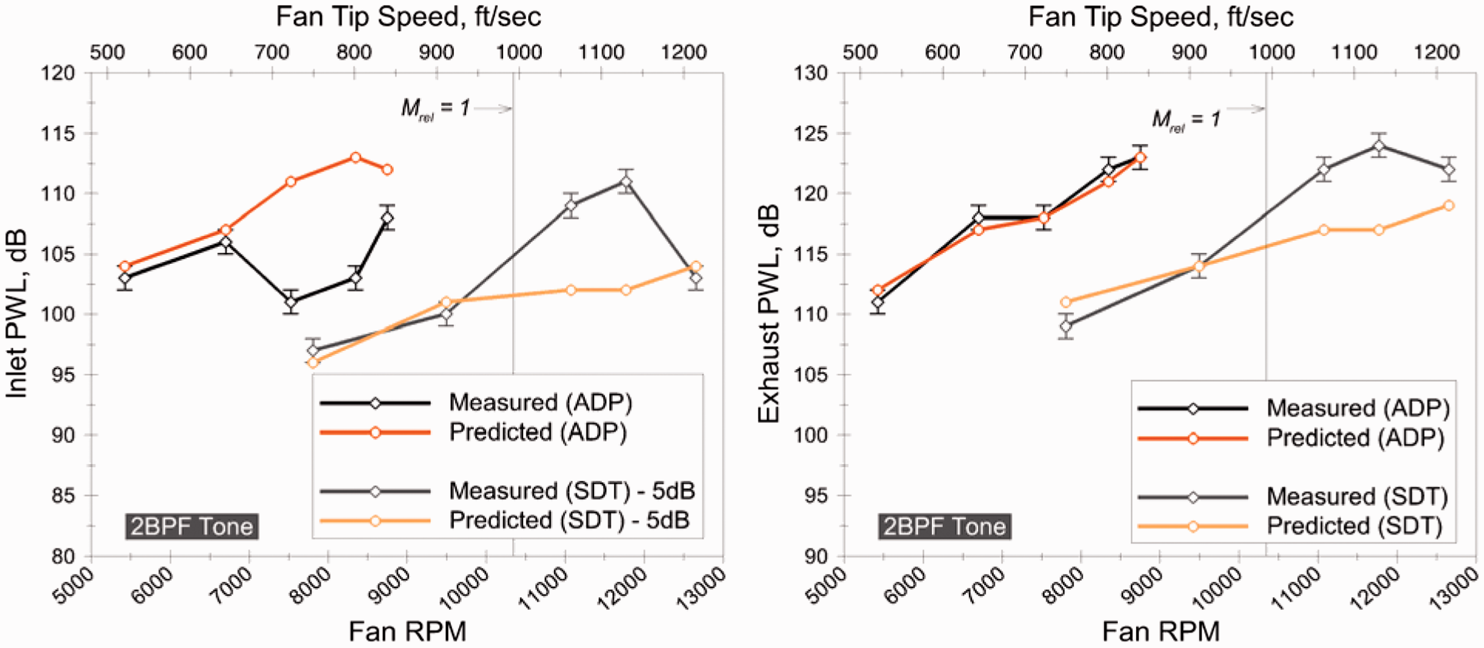
Comparisons with a R/S analytical model
At this point, we digress to examine the validity of employing the classical plug-flow duct mode description that is typically used in analytical or semi-analytical models of the R/S interaction tone noise. Recall that, in contrast, LINFLUX relies on numerically computed swirl or shear flow duct modes to represent the upstream and downstream propagating acoustic waves. To ensure a valid comparison of the results between the two types of duct mode descriptions, we have used the three-dimensional unsteady loading distributions on the OGV computed by LINFLUX as well as the three-dimensional geometry of the vanes as input to the analytical model. Recall that the analytical/semi-analytical models of R/S interaction noise typically rely on highly simplified descriptions of the OGV loading and geometry as well as on the analytical duct mode description. The goal here is to eliminate the limitations imposed by the simplified loading and geometry and focus solely on the effect of the duct mode description on the predicted mode levels.
The mathematical derivation of the frequency-domain analytical formula for calculating the acoustic field generated as a result of rotor wake impingement on the OGV is fairly straightforward and can be readily found in the literature. Here, we shall use the formula derived in literature
34
(equation 4.25):
n




The acoustic pressure 
If the distribution of the aerodynamic pressure f on the vane surface is known, the integration in equation (1a) can be explicitly carried out and the tone sound field inside the duct resulting from R/S interaction can be computed. As was stated earlier, we have used the three-dimensional geometry of the vane and the associated loading distributions that were computed with LINFLUX for that purpose. In fact, for convenience, we have used the vane surface grid from the LINFLUX simulations for calculating the surface integral in equation (1a). The SPLs and PWLs calculated by LINFLUX and those form the analytical model (i.e., equation 1a) for all the propagating modes (as determined by each model) are listed in Tables 6 through 9. The LINFLUX levels are the same as those listed in Tables 3 and 4. The analytical model levels are underlined for clarity.
The mode SPL comparisons indicate that, save for incidental agreement in a few instances, there is no discernable pattern of agreement between the LINFLUX and analytical mode results in either the upstream or downstream directions. The comparison is only marginally better for PWL in the upstream direction. However, in the downstream direction, there is much more consistent agreement between the PWL computed using LINLFUX and the analytical model results for a large number of modes or, at least, for the modes with the highest power levels. These comparisons suggest that for the purpose of computing the SPLs, the plug-flow assumption does not correctly model the modal content (i.e., the amplitudes and phases) of the tonal sound field inside the fan duct (upstream or downstream). This despite that fact that the tone power levels are reasonably well-predicted in the downstream direction using the classical mode theory if the vane surface pressures are accurate. These observations are reconcilable by noting that the PWL is a global (i.e., an integrated) quantity whereas the SPL is, in a sense, a local quantity. On the basis of these results, it is expected that on the basis of the tone power level (i.e., the sum of power levels in all the propagating modes), there would be a good agreement between the LINFLUX predictions and the analytical model predictions in the downstream direction. That is indeed the case as shown in Figure 11. The agreement in the downstream direction is quite good, whereas it is only marginal for the upstream direction.
Comparisons of predicted 2BPF tone power levels using the LINLFUX and analytical rotor–stator interaction models (equation 1a) for advanced ducted propulsor and source diagnostic fans test across their respective tip speed regimes. The inlet comparisons are shown on the left and exhaust comparisons on the right. The LINFLUX levels are the same as those in Figure 10. BPF: blade passing frequency.
These comparisons suggest that, whereas the plug-flow mode description in the upstream direction substantially misrepresents the physics of the swirling flow duct modes, in the downstream direction (where there is mostly shear flow) it does seem to model the acoustic power reasonably well. Of course, the principal reason for the good agreement is that the source amplitudes (i.e., the vane surface pressure distributions) are the same in both cases. The comparisons would not be nearly as good if a simpler source model (such as the flat plate strip analysis) was used to calculate the unsteady loading on the vanes in the analytical model. The salient point here is that the three-dimensional high-fidelity calculation of the vane surface pressure is crucial in developing a robust and accurate model for predicting the R/S interaction tone levels.
Sideline tone directivities
In the previous section, data–theory comparisons could only be carried out on the basis of PWL. In this section, we have used the exhaust SPLs computed by LINFLUX as input to an acoustic radiation model and projected them to the sideline locations in the wind tunnel where tone SPL had been measured in order to carry out a data–theory comparison on the basis of SPL. We have used an aft-duct radiation code developed by Eversman 50 for that purpose. This code is based on a frequency-domain, finite element formulation for the problem of acoustic radiation from an axisymmetric exhaust duct. The Eversman code solves weighted residual formulations for the mean flow and acoustic perturbations. To calculate a solution, in addition to the geometry of the exhaust duct (which must include the aft nacelle profile), the in-duct acoustic pressure distribution is needed at an appropriate axial plane, which serves as the input plane to the computational domain for the Eversman code. In this study, the input plane is taken to be the outflow boundary of the LINFLUX computational domain. The acoustic pressure specification in the Eversman code is accomplished via the analytical duct mode description given by equation (1c) using only the cut-on modes in one circumferential mode m at a time. Note that, only the pressure specification at the boundary is in terms of the classical duct modes. The subsequent evolution of the acoustic modes in the Eversman code is on the basis of a nonuniform mean flow, which depends on both the axial and radial coordinates. It should be noted that the mean flow, which is computed as part of the solution, is modeled as irrotational.
The presence of the nozzle shear layer poses special challenges as the dynamic of a real shear layer is highly complex and beyond the scope of the theory underlying the Eversman code. As a result, some simplifications are necessary to make the problem tractable. The shear layer is assumed infinitely thin and extending a finite distance downstream of the nozzle and terminating well before the end of the computational domain. Where it is assumed to exist, the shear layer marks the boundary between an “inner” and an “outer” flow region. The inner flow region is taken to be an extension of the exhaust duct flow and the outer flow region encompasses the rest of the external computational domain. The velocity potential is discontinuous across the shear layer, but becomes continuous when the shear layer ends. The inner and out flows are permitted to mix on a potential flow basis downstream of the shear layer termination point. The extent of the shear layer is chosen to provide acoustic wave refraction across the layer while minimizing the effect of the artificial flow mixing on the acoustic waves. The presence of the shear layer also necessitates the specification of two continuity conditions along the layer. These are the continuity of the acoustic pressure and the continuity of the shear layer displacement. Under these conditions, the layer effectively behaves as an impermeable boundary to the mean flow, but transmits the acoustic perturbations across by virtue of its local motion (see literature 50 ).
Because the theory models the aft-radiated noise, the computational domain does not include the inlet region either internal or external to the fan duct. Inside the fan duct, the domain begins at the outflow boundary of the LINFLUX computational domain. External to the fan duct, a “baffle” is introduced to isolate the aft-radiated acoustic field from the inlet. The baffle location is chosen sufficiently far away from the nozzle to minimize its influence on the solution. Additionally, the aft centerbody is shortened and tapered in order to reduce the size of the computational domain and improve the quality of the finite element mesh. The recommended rule for specifying the mesh density in the Eversman code is that there should be at least five elements per wavelength in the principal direction of propagation, which is axial in the duct and radial in the external domain. The formula relating the number of elements per wavelength ( Top: The domain for exhaust radiation calculations begins downstream of the OGV at the location labeled “input plane” and ends at the “baffle” external to the nacelle. Bottom: The finite element grid used in the radiation calculations is comprised of multiple regions starting inside the duct and extending to the outermost boundary. The red dot marks the origin for the Eversman code computational domain and grid. The black dot marks the origin used in the wind tunnel tests and sideline angle comparisons shown in later figures. OGV: outlet guide vane.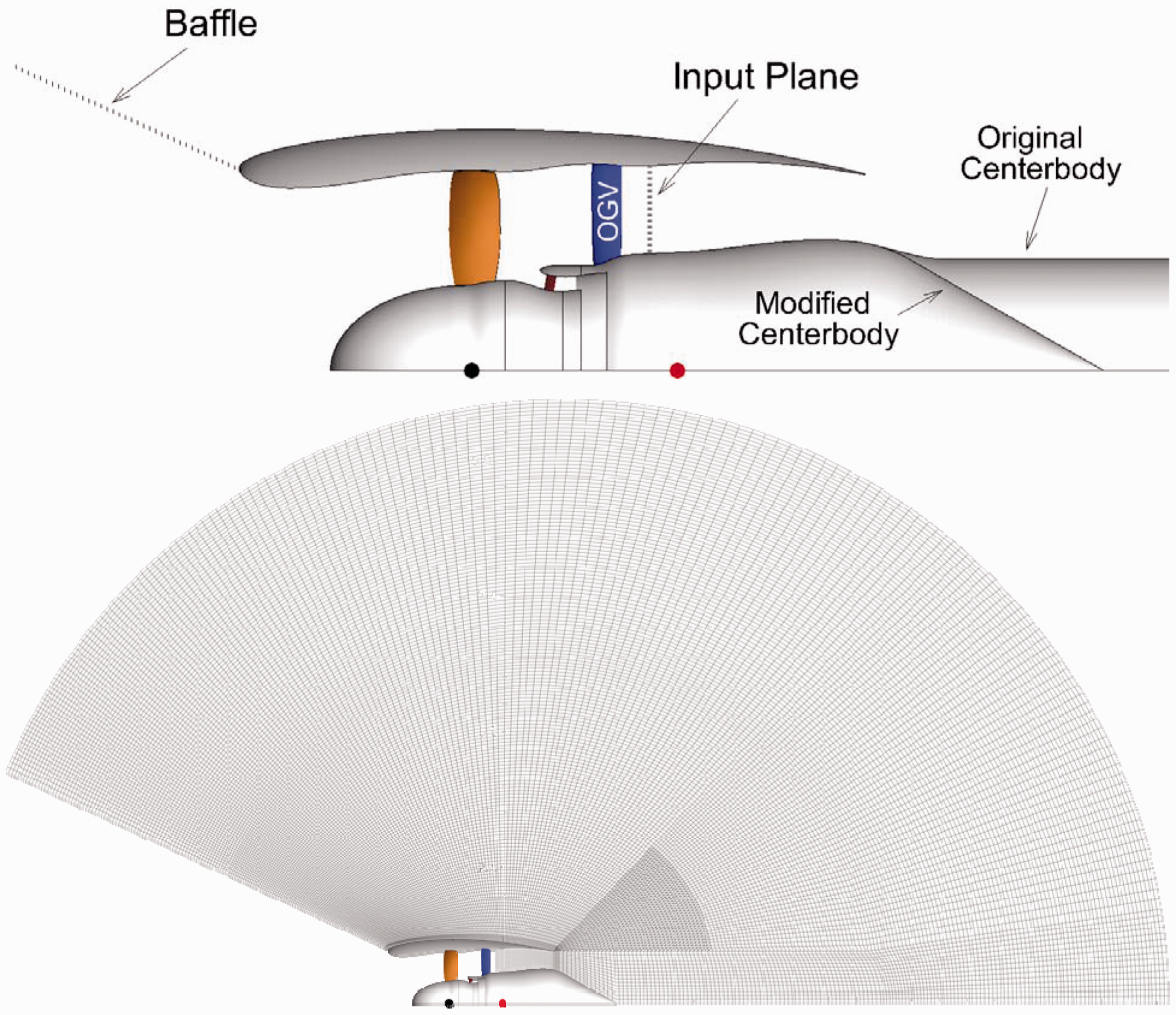
Finally, it should be noted that to ensure a good-quality finite element mesh, the coordinate origin had to be shifted downstream (the red dot in Figure 12) from its normal position (the black dot in Figure 12), which is the stacking axis of the fan. The shift used here is equal to one input plane radius, which is
For the radial mode amplitude specification at the input plane, theoretically, the pressure distribution at the LINFLUX outflow plane should be expanded in the terms of the radial modes of the classical theory. In other words,

The aft radiation calculations were carried out for both fans, but for the SDT fan, the calculations were restricted to the subsonic tip relative speeds because for the supersonic tip relative speeds, the contribution of the rotor-locked pressure field is missing from the predicted in-duct levels (see Figure 10 and the associated discussion).
We begin the presentation of the sideline results with Figure 13, which shows the predicted directivity of the 2BPF tone on the 89.3″ (2.27 m) sideline for the ADP fan at the 8750 r/min. The abscissa is the sideline (geometric) angle and the ordinate is the SPL on the sideline. The purpose of this plot is to show the relative contributions of the constituent (propagating) radial modes to the overall tone level and the way the relative phase among the modes can affect the tone directivity.
Sideline directivity of individual propagating radial modes for ADP at 8750 r/min. The calculations were carried out using the LINFLUX predicted mode amplitudes as input to the Eversman radiation code. The curve labeled “Total” is the 2BPF tone directivity, which is comprised of all propagating radial modes. ADP: advanced ducted propulsor.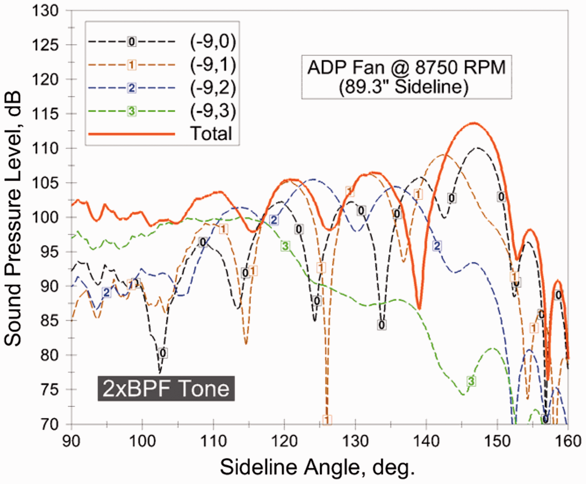
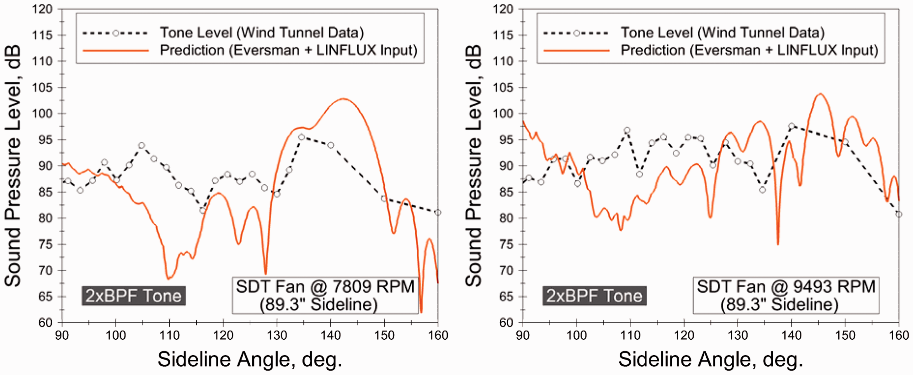
The comparisons of the predicted and measured sideline SPLs for the 2BPF tone are shown in Figure 14 for the ADP fan and in Figure 15 for the SDT fan. We remind the reader that the radiation calculations were carried out for all speeds for ADP, but only for two subsonic tip relative speeds for SDT. As indicated earlier, the sideline levels were computed using the input mode levels calculated by the LINFLUX code. It should be noted that the angular resolution of the computed directivities is far higher than the measured directivities (0.1° vs. 2.5°). As such, the definition of the peaks and valleys in the SPL directivity are much better resolved in the computations than they are in the measurements. As a result, the relatively coarse measured directivities do not necessarily represent the true behavior of the tone directivities if they were viewed on finer angular increments. In spite of this limitation in the data, for the most part, the data–theory agreement is reasonable especially for sideline angles greater than 120°. While there are substantial discrepancies at some sideline angles for some speeds, the overall trends with speed are well captured.
Comparisons of predicted and measured 2BPF sideline sound pressure levels for the ADP fan for all operating conditions considered in this study. In all cases, mode amplitudes from LINFLUX were used as input to the Eversman radiation code. ADP: advanced ducted propulsor; BPF: blade passing frequency. Comparisons of predicted and measured 2BPF sideline sound pressure levels for the SDT fan at the subsonic tip relative speeds. LINFLUX mode amplitude predictions were used as input to the Eversman radiation code. BPF: blade passing frequency; SDT: source diagnostic test.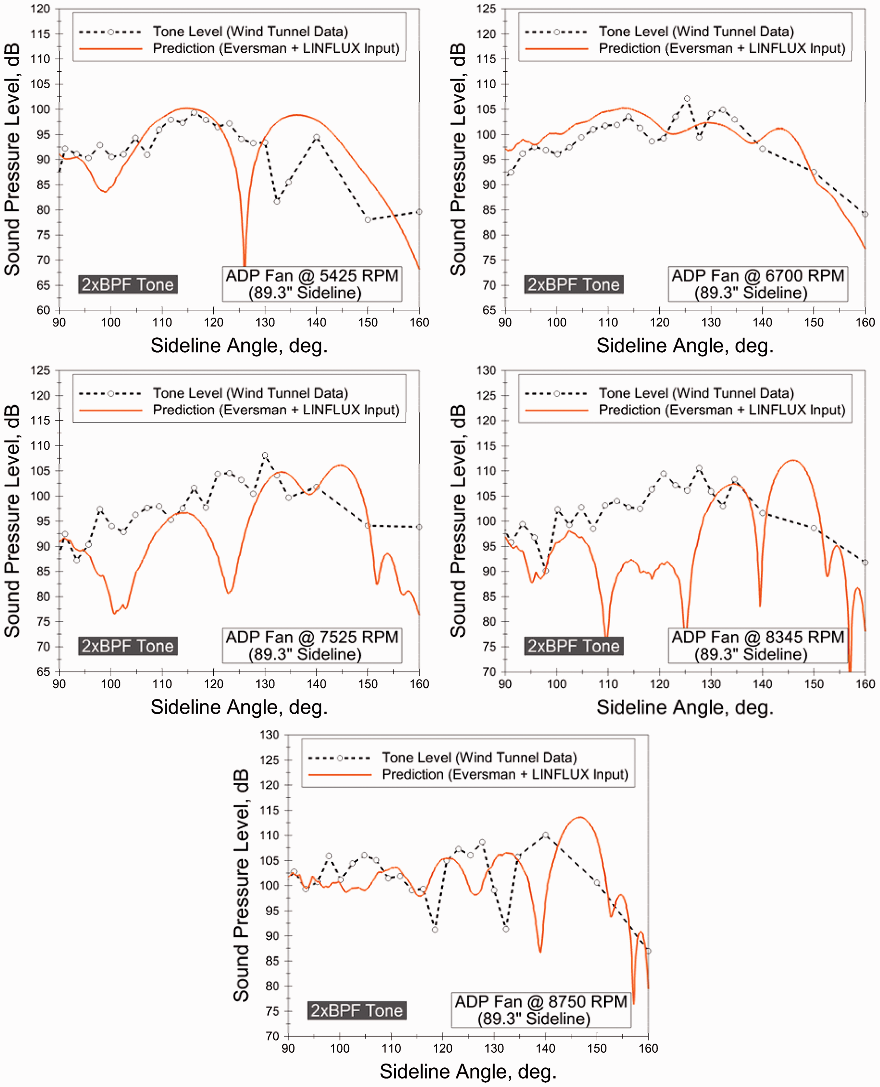
Generally speaking, the comparisons are encouraging for several reasons. First, the chain of calculations, from the RANS flow simulations for estimating the rotor wakes, to the linearized Euler simulations for computing the in-duct levels, to the linearized potential field simulations for computing the exhaust acoustic radiation to the sideline, has not been calibrated in any way. Second, as Figure 13 indicates, the nature of the tones is such that they are dependent on the relative phases of their constituent radial modes requiring a precise prediction of the modal phases, which is a difficult task especially in view of the next two observations. Third, an examination of the sideline measurements of the tones in the wind tunnel indicates that the fan tones are inherently “unsteady” due to the slight, but ever present, variations in the fan rpm resulting from fluctuations in the wind tunnel environment. The ADP and SDT fan tests in the 9 ft × 15 ft wind tunnel were conducted by holding the target rpm, known as the corrected rpm (denoted by RPMc) constant. RPMc is related to the physical (i.e., actual) rpm (denoted by RPMa) via the relationship
Conclusions
The principal conclusion of this work is that, based on the results of previous sections, it is feasible to predict the fan exhaust tone levels generated by the R/S aerodynamic interaction using purely numerical models without reliance on empiricism or code calibration. To put it more precisely, the results indicate that starting with the geometry of a fan stage one can combine RANS methods and linearized inviscid methods to compute, accurately, the tone power levels resulting from the R/S interaction across the range of the fan operating conditions. The caveat being that the R/S interaction mechanism must be the dominant source of tone noise, which is the case when the fan tip relative speed is subsonic.
To extend the analysis to the supersonic tip relative speeds, one must also include the contribution from the rotor-locked pressure field scattered by the OGV. The rotor-locked pressure field is evanescent at subsonic tip relative speeds and is ignored, but at supersonic tip relative speeds, it is propagating and becomes significant and possibly even dominant. That contribution could be computed as follows. One could use RANS methods to calculate the rotating rotor-locked pressure field of the rotor. Then one could expand the pressure field in terms of the acoustic modes of the swirling base flow region between the rotor and the stator. The interaction of these acoustic modes with the OGV could then be computed using the LINFLUX or similar codes. The expansion of the rotor-locked pressure filed in terms of the numerically computed swirling base flow modes is not a trivial exercise, but one that is feasible with careful implementation of the steps involved.
Also, if an accurate and reliable three-dimensional model of rotor acoustic transmission could be developed, it would be possible to use the same suite of tools to predict the inlet tone levels more accurately as well. That could potentially be done using linearized inviscid models (like LINFLUX) to calculate the interaction of the upstream OGV tones with the rotor. For the purposes of such an analysis, and as a good approximation, the rotor mean flow field could be assumed inviscid. In such calculations, features like the rotor tip flow could be ignored as they should not greatly affect the acoustic transmission physics.
As the results of the subsection titled Comparisons with a R/S analytical model clearly demonstrate, another significant conclusion is the importance of using three-dimensional descriptions of the geometry and flowfield for accurate predictions of constituent mode content of the fan tones. Analyses based on simplified OGV geometry (e.g., twisted flat plates), quasi-3D aerodynamic response models (e.g., strip analysis), or plug flow duct mode expansion fail to describe the physics of the problem sufficiently accurately to provide acceptable results that can be relied on for design and analysis purposes. In contrast, the more realistic descriptions of the OGV geometry and flowfield provide excellent estimates of the tone power levels inside the duct, especially for the exhaust tones.
Additionally, the results from the subsection titled Sideline tone directivities indicate that despite the inherently complex nature of tone directivity outside of the nacelle, linearized methods could still provide an acceptable description of the trends with the operating condition and, for a range of sideline angles, even provide quite reasonable estimates of the tone SPLs. These predictions could potentially be improved by modeling the shear layer refraction more accurately, which would require more rigorous treatment of the shear layer physics. Such treatment may well necessitate the inclusion of the shear layer spreading and the use of rotational flow models.
Finally, this study was narrowly focused on one frequency (namely, the second harmonic of the blade passing frequency) in order to demonstrate the entire modeling chain in great deal of detail. However, since the underlying R/S interaction mechanism is the same for other harmonics of the BPF, those tones should be equally amenable to the application of the same suite of tools. Naturally, the computational grid resolution and computer resource requirement would grow as the harmonic order increases and the tone amplitude decreases, which is typically the case for the subsonic fans.
Footnotes
Declaration of conflicting interests
The author(s) declared no potential conflicts of interest with respect to the research, authorship, and/or publication of this article.
Funding
The author(s) disclosed receipt of the following financial support for the research, authorship, and/or publication of this article: This work was supported by the NASA Advanced Air Transportation Technology Project.