Computation of the self-noise of a controlled-diffusion airfoil based on the acoustic analogy

Abstract

The self-noise of a controlled-diffusion airfoil is computed with several numerical techniques based on the acoustic analogy and involving different degrees of approximation. The flow solution is obtained through an incompressible large eddy simulation. The acoustic field as described by Lighthill’s analogy is computed with a finite element method applied to the exact airfoil geometry, and this solution is compared with results based on a half-plane Green’s function. This problem behaves as a classical trailing-edge noise problem for a wide range of frequencies; however, other mechanisms of sound production become significant at high frequencies. The results highlight the relative strengths and weaknesses of quadrupole- and dipole-based formulations of the acoustic analogy based on incompressible Computational Fluid Dynamics (CFD) results when applied to wall-bounded turbulent flows.

Keywords

Trailing edge noise controlled diffusion airfoil acoustic analogies

Introduction

Trailing-edge noise or broadband self-noise, caused by the scattering of the boundary-layer disturbances into acoustic waves, occurs at the trailing edge of any airfoil surface. This noise mechanism is the minimum sound that a lifting surface would produce in absence of other sound mechanisms as turbulence interaction at the leading edge or possible trailing-edge vortex shedding due to the trailing-edge bluntness. This mechanism is responsible for a significant proportion of the noise emitted by low-speed cooling fans in automotive applications,¹ wind turbines,^2,3 and high-lift devices.^4,5

Different theories have been proposed for the modeling of trailing-edge noise.⁶ More recently, generalizations of some of these theories have been proposed to take into account the noncompactness effects of a finite chord length. This is the case of the extension to Ffowcs Williams and Hall half-plane Green’s function (GF)⁷ proposed by Howe,⁸ or of the work of Moreau and Roger^9,10 based on Amiet’s theory.¹¹ In the last years, detailed unsteady flow computations have been applied to predict trailing-edge noise, typically, although not always, in combination with an acoustic analogy. Early examples of such works can be found in the literature.^12–14

The use of incompressible flow computations as a basis to define equivalent sources using the acoustic analogy has been object of some attention in the literature. In general, a GF that satisfies the correct hard-wall boundary conditions (BCs) of the problem on solid boundaries is necessary. For an arbitrary geometry, this GF can be computed numerically, or, equivalently, the acoustic equation with the correct BCs for the acoustic variable(s) can be solved numerically. Such an approach was applied successfully to trailing-edge noise prediction by Oberai et al.,¹⁵ based on a finite element method (FEM) to solve Lighthill’s equation,¹⁶ and by Khalighi,¹⁷ based on a boundary element method.

Methods based on surface-distributed sources defined over the boundary also need to satisfy the correct hard-wall acoustic BCs on solid boundaries; otherwise, large errors can arise for noncompact geometries. This is the case of Curle’s analogy,¹⁸ later generalized by Ffowcs Williams and Hawkings for surfaces in arbitrary motion.¹⁹ Curle’s solution to Lighthill’s equation is based on a free-field GF, because it assumes that the flow solution already satisfies the correct acoustic BCs at the wall. If the flow is incompressible, this condition is not met, which can lead to erroneous acoustic predictions when the solid body dimensions are not small compared to the wavelength, as illustrated in the literature.^15,20 To overcome this issue, Schram²¹ proposed to introduce an ad hoc explicit distinction between aerodynamic and acoustic pressure fluctuations. More recently, an alternative approach consisting in using Curle’s sources to define acoustic Neumann-type BCs was proposed.²² Results presented as a proof of concept on a 2D geometry suggest that this approach is capable of capturing the physical behavior of trailing-edge noise as long as the scattering by the wall (Curle’s dipole sources) is the dominant contribution to the sound production.

The present work is inscribed in that line and aims at contributing to the field by exploring in deeper detail the respective contributions of dipoles and quadrupoles to the noise emitted by the flow developing over a controlled-diffusion (CD) thin airfoil, which has already been studied in previous works, both experimentally and numerically.^23–28 The general framework is based on Lighthill/Curle acoustic analogies, addressing in particular the respective strengths and weaknesses of dipole- or quadrupole-based formulations when an incompressible flow model is used as an input and the chord is noncompact. Different implementations of these analogies are presented, for different choices of GFs. Results obtained using the analytical GF derived by Ffowcs Williams and Hall and a finite element solver are compared, demonstrating the respective merits of the various formulations in terms of efficiency and capability to highlight the sound generation mechanisms over a broad range of frequencies.

The outline of this paper is as follows: the next section presents the case and describes the incompressible flow computations; “Methodology for the acoustic study” section describes the approaches applied for the numerical acoustic study; “Results of the acoustic study” section contains the discussion of the acoustic prediction results obtained with the different approaches and, the final section presents the conclusions of the study. Appendix 1 is included containing a study of the sensitivity of the finite element results with respect to several modeling aspects (size of the source region and truncation error correction, averaging over several time windows, finite element discretization).

Case description and flow simulations

The airfoil geometry considered in the present work is related to the Valeo automotive cooling module illustrated in Figure 1 (left). The rotor is represented together with the heat exchanger placed upstream, the convergent guiding the flow to the rotor section, the motor and the downstream stator that is also holding the rotor. The selected blade profile is a CD airfoil designed by Valeo. The CD airfoil is the shape that is found at the midspan region of the fan blade and this profile is used for the pitchline (chord line at the designated angle of attack) analysis in their preliminary design process. CD airfoils are a class of cambered airfoil that employs specific characteristics to carefully control the flow around the airfoil surface. The profile has a 4% thickness to chord ratio and a camber angle of 12°.

Figure 1.

(Left) Representation of the complete automotive cooling module and (right) the large wind tunnel of ECL. ECL: Ecole Centrale de Lyon.

The CD airfoil was investigated experimentally in the large anechoic wind tunnel of Ecole Centrale de Lyon (ECL), shown in Figure 1 (right). The measurements include wall pressure measurements (mean and spectra), hot wire measurements, and far-field microphones measurements.^23–25 Additional measurements were performed in the 0.61 m² tunnel of the Turbulent Shear Flow Laboratory at Michigan State University reproducing the flow conditions found in the ECL wind tunnel. The airfoil mock-up has a 0.134 m constant chord length (c) and a 0.3 m span (L). It is held between two horizontal side plates fixed to the nozzle of the open-jet wind tunnel as shown in Figure 1 (right). These plates are 0.25 m (≈1.85 c) apart and the width of the rectangular jet is 0.5 m (≈3.7 c). As shown by Moreau et al.,²⁹ this aspect ratio insures that the 3D effects at midspan are therefore minimized. The computations presented here are run with a speed $U_{\infty}$ = 16 m/s, which corresponds to a Reynolds number based on the airfoil chord length Re_c = 1.6 × 10⁵, and the angle of attack is 8°. For this flow condition, the turbulence intensity at the outlet nozzle always remains lower than 1% in the facility. The CD airfoil mock-up is equipped at midspan with 21 flush-mounted electret remote microphone probes (RMP).⁴ The RMPs measure both the mean and fluctuating pressure within a frequency range of 20–25 kHz.²⁴ Hot wire measurements were collected in the airfoil wake and across the boundary layer of the airfoil.^23,25 The pressure and velocity measurements are used to validate the large eddy simulation (LES) flow data used in the present study and summarized below (see Christophe et al.³⁰ for further details). The far-field noise is measured using a single B&K 1/2″ Type-4181 microphone in the midspan plane at a distance of 2 m from the airfoil trailing edge.

As in previous studies,^13,31,32 a similar strategy has been used to take into account that the airfoil is immersed in a jet of finite width, which is deflected by the circulation created by the airfoil, having an impact on the airfoil loading and the corresponding noise created. In order to match closely the experiments with the LES computations around the airfoil, the following procedure is used. As shown by Moreau et al.,²⁹ a 2D Reynolds-averaged Navier–Stokes (RANS) simulation of the complete open-jet wind tunnel configuration including the nozzle, the airfoil, and part of the anechoic chamber is first required to capture the strong interaction between the jet and the CD airfoil and its impact on the airfoil loading at any incidence. The full RANS simulation provides velocity BCs for the smaller LES truncated domain which is embedded between the two boundary shear layers of the jet. The preliminary RANS computation is performed using the shear-stress transport $k - ω$ turbulence model, with second-order accurate solution for all variables. A small turbulent intensity about 0.7% corresponding to the experiments is imposed at the nozzle inlet. The low Reynolds number Re_c and the larger jet width to chord ratio in the present experiment allow a LES computational domain around the full airfoil.

The size of the LES computational domain is $4 c$ in the streamwise (x) direction and $2.5 c$ in the crosswise (y) direction. The resulting spanwise cut of the LES grid is a single block-structured C-mesh, with 960 × 84 cells in the present computation. The near-wall grid spacing, except near the leading edge, reaches maximum values of $x + = 34, y + = 1.1$ on the airfoil surface. This 2D mesh is then extruded in the spanwise direction with a width of $0.1 c$ and with a discretization of 64 cells. The spanwise extent and the spanwise discretization influence have been verified by Christophe et al.,³⁰ through spanwise correlations and coherences. The LES computation is based on the spatially filtered incompressible Navier–Stokes equations with the dynamic Smagorinsky subgrid-scale model. Equations are solved with the finite volume solver OpenFoam 1.5. Numerical schemes are second-order accurate in space and time. A time step of $Δ t' = Δ {tU}_{0} / c = 2.10 - 4$ is used, yielding a Courant-Friedrichs-Lewy (CFL) number below 0.6. The computation was run for 5 $t'$ ( $t' = {tU}_{0} / c$ ), before a statistically steady state was reached and mean values were collected. Airfoil surface pressure and flow volumetric velocities in the complete domain were then acquired for a period of $5 t'$ sampled every 10 time steps, corresponding to a sampling rate of about 60 kHz. Further details about the flow computation and validation can be found in Christophe et al.³⁰

Methodology for the acoustic study

Overview of the approaches used in this work

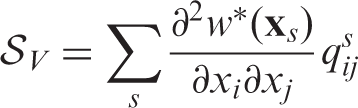
All the acoustic prediction methods applied in this work aim at providing a solution for Lighthill’s equation,¹⁶ with sources obtained from the incompressible flow computations described in “Case description and flow simulations” section. The considered flow around the airfoil is assumed incompressible in the source region and homentropic, and viscous effects are neglected. With these hypotheses, Lighthill’s equation expressed in Fourier domain can be written as

\nabla 2 \overset{\land}{p} + k 2 \overset{\land}{p} = - \frac{\partial 2 \overset{\land}{ρ_{0} u_{i} u_{j}}}{\partial x_{i} \partial x_{j}}

(1)

where the hat

\overset{\land}{\cdot}

over a variable or product of variables indicates a Fourier component, and where

\overset{\land}{p}

is the acoustic pressure, u_i is the flow velocity component, and ρ₀ is the reference density in the source region.

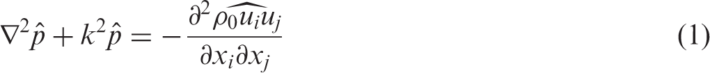
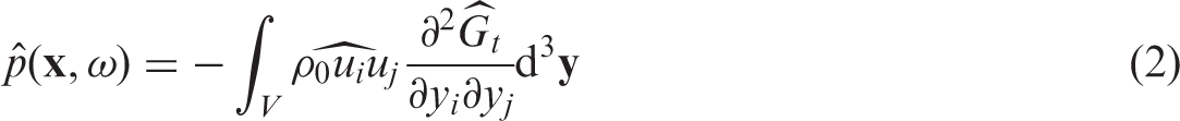
In the presence of solid walls, one alternative for solving equation (1) is to use a GF that is tailored to the geometry of the boundary, i.e. that satisfies the correct BCs of the problem. Given a tailored GF G_t, the acoustic pressure outside the source region is given by the following volume integral over the source region V

\overset{\land}{p} (x, ω) = - \int_{V} \overset{\land}{ρ_{0} u_{i} u_{j}} \frac{\partial 2 \overset{\land}{G_{t}}}{\partial y_{i} \partial y_{j}} d 3 y

(2)

In this equation, the source term is given by a volume distribution of quadrupole sources.

Alternatively, equation (1) can be solved numerically, forcing the acoustic variable to satisfy the correct hard-wall conditions at the boundary. In this work, Lighthill’s equation (1) is solved with a FEM, the details of which are presented in “Finite element models” section.

Curle’s solution¹⁸ to Lighthill’s equation in the presence of walls makes use of a free-field GF and models the sources due to the interaction of the turbulence with the surface as surface-distributed dipoles. For a fixed rigid surface S, and under the same assumptions as above (homentropic flow, negligible viscous effects also at the walls, incompressible flow in the source region), Curle’s solution can be expressed as

\overset{\land}{p} (x, ω) = - \int_{S} {\overset{\land}{p}}_{f} \frac{\partial \overset{\land}{G}}{\partial y_{j}} n_{i} d 2 y - \int_{V} \overset{\land}{ρ_{0} u_{i} u_{j}} \frac{\partial 2 \overset{\land}{G}}{\partial y_{i} \partial y_{j}} d 3 y

(3)

where G is the free-field GF, p_f is the flow pressure, and n_i is a component of the normal unit vector n directed toward the exterior of surface S (i.e. outside the volume V). Equation (3) highlights that the solution to Lighthill’s equation can be seen as the sum of two contributions: the sound produced due to the interaction of the wall with turbulence, modeled with surface dipole sources and the sound due to free turbulence, modeled through quadrupole sources. When the surface is acoustically compact (or the sound production is concentrated around an acoustically compact feature of the surface like an edge), dipole noise dominates over free quadrupole noise and the second integral can be neglected for low Mach numbers

\overset{\land}{p} (x, ω) \approx - \int_{S} {\overset{\land}{p}}_{f} \frac{\partial \overset{\land}{G}}{\partial n (y)} d 2 y

(4)

However, if the flow pressure corresponds to an incompressible flow description and if the surface is not acoustically compact, Curle’s solution can become inaccurate while being mathematically exact. The reason is that it assumes that the surface pressure includes the acoustic scales and satisfies a priori the correct acoustic BCs on the surface. This is, however, not guaranteed when the pressure is given by an incompressible flow computation, which lacks acoustic information.

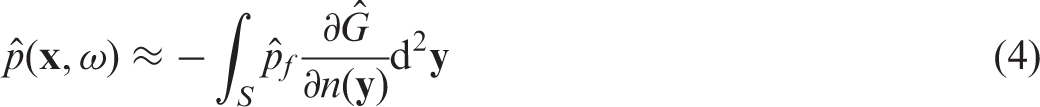
To overcome this limitation, Curle’s dipoles can be used to define BCs of the acoustic problem, which can then be solved numerically.²² The rationale behind this is that the aerodynamic pressure should be sufficient to characterize the sources of sound production if dipoles are dominant, while the missing acoustic information on the surface can be computed numerically, provided that the acoustic pressure is forced to satisfy appropriate acoustic BCs on the surface. In particular, it can be shown that the solution of the homogeneous acoustic equation

\nabla 2 \overset{\land}{p} + k 2 \overset{\land}{p} = 0

(5)

with Neumann BCs on S defined as

\frac{\partial \overset{\land}{p} (x, ω)}{\partial n (x)} |_{S} \approx - \frac{\partial}{\partial n (x)} \int_{S} {\overset{\land}{p}}_{f} \frac{\partial G (0)}{\partial n (y)} d 2 y

(6)

where

G (0)

is the free-field GF of the Laplace equation, yields more accurate results than Curle’s analogy if the flow pressure p_f corresponds to an incompressible flow description.²² Note that for this approach to be accurate, dipole sources should be dominant.

The purpose of this acoustic study is to apply and compare these different approaches to gain insight on the different mechanisms of sound generation on the CD airfoil. Table 1 summarizes the approaches used here. While they all share the same acoustic propagation operator, they vary in the way sources are modeled (quadrupoles, dipoles, or dipoles as BCs), the method (GF or numerical solution of the acoustic equation based on a FEM), and the treatment of the geometry (discretization of the exact geometry or approximation of the airfoil by a half plane).

Table 1.

Approaches for the acoustic prediction.

	Method	Sources	Geometry
Curle’s solution	Free-field GF	Surface dipoles	Exact
FEM with dipoles	FEM	Surface dipoles as BCs	Exact
FEM with quadrupoles	FEM	Volume quadrupoles	Exact
Half-plane GF	Half-plane GF	Volume quadrupoles	Half plane

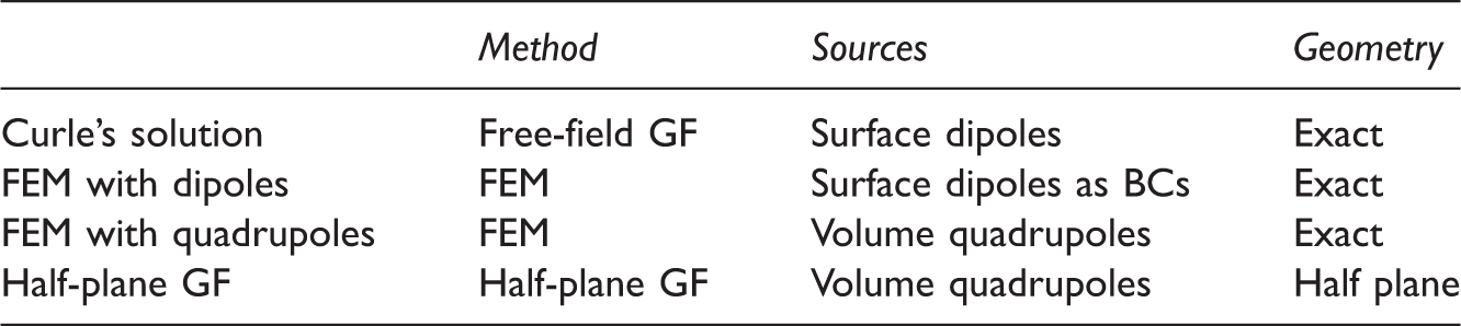
BC: boundary condition; FEM: finite element method; GF: Green’s function.

Curle’s solution is based on equation (4), with the flow pressure mapped from the CFD mesh onto a surface acoustic mesh where the surface integral is evaluated. More details about the discretization of the airfoil surface are provided in “Discretization of the geometry” section.

As for the finite element computations, “Finite element models” section provides more details about the models and schemes. The FE computation with dipoles uses equation (6) to transform them into Neumann BCs of the acoustic equation, while the FE computation with quadrupoles is based on a discretization of the tensor $ρ_{0} u_{i} u_{j}$ .

Finally, more details of the solution with the half-plane GF can be found in Christophe et al.,³⁰ which follows the same approach used in the literature.^25,26

Discretization of the geometry

A surface mesh with around 87,000 triangular elements and 43,500 nodes discretizing the full airfoil wall is shown in Figure 2. This mesh includes the whole span of the airfoil ( $\approx 2.21 c$ ). In practice, the CFD mesh only covers a span length of $0.1 c$ , and thus the sources are only available in a relatively narrow portion of the airfoil mesh, which is centered at the airfoil midspan plane. This CFD span length of $0.1 c$ is larger than the flow correlation length, and therefore, if the span is divided into segments of this length, these can be considered as uncorrelated. Therefore, a simple scaling of the results obtained with the available sources, using the ratio of full span length to CFD span length ( $= 22.1$ ), is enough to account for the effect of sources along the full airfoil span.

Figure 2.

Top view and lateral view of the airfoil surface mesh.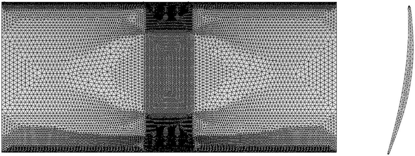

The surface mesh is refined around the center of the span, to capture near-field effects of the sources more accurately and also to reduce interpolation errors of the dipole sources on the acoustic mesh. The mesh is also refined around both trailing and leading edges, which are regions where the solution can display stronger gradients. A sensitivity study of Curle’s solution with respect to the mapping scheme of the flow pressure was carried out. The results were not very sensitive to the properties of the mapping scheme (such as whether it forced or not the conservation of the surface pressure integral), indicating that the surface mesh is fine enough to capture accurately the flow gradients that are relevant for the acoustic computation.

This surface mesh is used to compute Curle’s solution (with zero-valued dipoles outside the CFD region). It is also used to build a volume mesh around it for the finite element computations. The FE mesh, shown in Figure 3, has around 759,000 tetrahedral elements and 150,000 nodes. “Finite element models” section provides more details about the finite element schemes and models.

Figure 3.

Midspan plane of the FE acoustic mesh. FE: finite element.

Finite element models

A weak form of the Helmholtz equation is solved numerically with the software LMS Virtual.Lab³³

\int_{Ω} \nabla w * \cdot \nabla \overset{\land}{p} d V - k 2 \int_{Ω} w * \overset{\land}{p} d V - \int_{Γ a} w * \nabla \overset{\land}{p} \cdot n d S + [NRBC]_{Γ ext} = S_{V}

(7)

where Ω is the computational domain and

w *

is the complex conjugate of the test function w, and where the terms

S_{V}

and

[NRBC]

depend on the volume-distributed sources and on the nonreflective boundary conditions (NRBC) applied on the external surface

Γ ext

, respectively.

The NRBCs are based on a perfectly matched layer³⁴ that starts on the external surface $Γ ext$ of the core FE mesh. The size and properties of the perfectly matched layer are automatically adapted by the software for each frequency to optimize its absorbing behavior.^35,36

In equation (7), the surface integral depends on the BCs used to characterize the airfoil surface $Γ a$ . In this work, only Neumann BCs are used. As explained above, computations with volume-distributed quadrupole sources as well as with dipole sources defined as BCs are carried out. The value of the Neumann BC on $Γ a$ and the term for the volume sources are in each of these cases:

Computations with dipole sources

\nabla \overset{\land}{p} \cdot n |_{Γ a} = \frac{\partial \overset{\land}{p}}{\partial n} |_{Γ a} \approx - \frac{\partial}{\partial n (x)} \int_{Γ a} {\overset{\land}{p}}_{f} \frac{\partial G_{0}}{\partial n (y)} d 2 y

as explained in “Overview of the approaches used in this work” section, and

S_{V} = 0

Note that to compute the Neumann BC from the flow pressure p_f an hyper-singular boundary integral must be evaluated. This is done here with the same technology applied to compute the hyper-singular operator in variational indirect boundary element methods, and can therefore have a significant cost in terms of computation time and memory requirements.

Computations with quadrupole sources:

\nabla \overset{\land}{p} \cdot n |_{Γ a} = 0

and

S_{V} = \sum_{s} \frac{\partial 2 w * (x_{s})}{\partial x_{i} \partial x_{j}} q_{ij}^{s}

where

x_{s}

is the source location corresponding to the centroid of each CFD cell (identified with the index s), and where

q_{ij}^{s}

is the integral of the source term in this CFD cell of volume V^s

q_{ij}^{s} = \int_{V s} \overset{\land}{ρ_{0} u_{i} u_{j}} d V

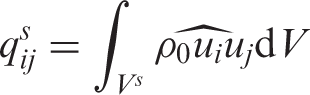
The quadrupole sources are defined in a subregion of the FE computational domain where most of the sound is produced. The influence of the extent of the source region is discussed in “Truncation of the quadrupole region” section of Appendix 1.

Discrete solutions in the space $C (0)$ of piece-wise differentiable continuous functions are sought for $\overset{\land}{p}$ . The shape functions are Lobatto functions of varying order, which is a function of the frequency and size of the elements of the acoustic mesh.^33,37 This is a strategy that allows using the same coarse acoustic mesh for the whole frequency range, while increasing the order locally for the coarsest elements only when the frequency is high and, therefore, the acoustic wavelength is small. Note that, in any case, solving the acoustic problem is in general significantly less demanding in terms of spatial resolution than solving the flow problem, which requires capturing small turbulent scales. Therefore, the acoustic mesh will tend to be much coarser than the CFD mesh, as is the case in the present computations. “FE discretization of the acoustic models” section in Appendix 1 presents a study of the sensitivity of the results to the order of the shape functions in different regions of the FE mesh.

The elements where the quadrupole source region is defined have always a fixed minimum order, which by default is taken as p = 3. The minimum order required is in any case p = 2, since the quadrupole sources require using the second derivatives of the shape functions. Note that the fact that the shape functions are defined in $C (0)$ involves that their derivatives are not necessarily continuous in the interface between elements, in spite of the fact that the quadrupole source term is based on their second derivatives. This requires that each of the discrete quadrupole sources is considered as located inside one element of the FE acoustic mesh, excluding its boundary.

It should be noted that the far-field points where the solution is measured are outside the FE computational domain. To obtain the acoustic field at these points, a Kirchhoff surface integral is computed on the external surface $Γ ext$ based on the FE solution.

The extent of the source region can have a significant impact on the accuracy of the acoustic results, especially when the source region is truncated abruptly.³⁸ In “Truncation of the quadrupole region” section of Appendix 1, a study of the sensitivity of the results to the extent of the source region is presented, as well as to the definition of spatial windows that are used to force the sources to decay gently toward the outlet to minimize the impact of spatial truncation errors. It is worth noting that the quadrupole source region is always well contained inside the FE computational domain and always several FE elements away from the external surface $Γ ext$ , where the Kirchhoff surface integral is computed and where the nonreflective acoustic BCs are defined. This prevents source near-field effects from adding numerical pollution to the acoustic solution.

Appendix 1 contains a study of the sensitivity of the FE results with respect to several numerical aspects of the FE models and source models.

Results of the acoustic study

This section discusses the results obtained with the approaches presented in “Overview of the approaches used in this work” section and compares them with the experimental measurements of Moreau and Roger. The results have been processed to make them comparable with the experiments. In particular, the sound pressure level (SPL) is computed as

SPL (x, ω) = 10 \log ((\frac{| \overset{\land}{p} (x, ω) |}{P_{REF}}) 2 \frac{Δ f exp}{Δ f CFD} \frac{L_{s}^{exp}}{L_{s}^{CFD}})

where the reference pressure is

P_{REF} = 210 - 5

Pa, Δf represents the frequency resolution, and L_s is the span length. As discussed in “Discretization of the geometry” section, the ratio of the span length of the real airfoil to the span length in the CFD simulation is

\frac{L_{s}^{exp}}{L_{s}^{CFD}} = 22.1

The experimental data are integrated in bins of width $Δ f exp = 8$ Hz. The frequency resolution of the numerical results depends on the length of the CFD time series, which has been divided for the FE computations in seven time windows of 500 timesteps (with 50% overlap) to allow for averaging. This yields a frequency resolution of $Δ f CFD = 118$ Hz.

All the results of the FE computations shown in this section have been averaged over the seven time windows, which represent each an individual numerical solution. For the Fourier transform of the flow data (pressure or quadrupole tensor $(ρ_{0} u_{i} u_{j})$ ), a Hann window has been applied on each time segment, scaled as to conserve energy for the SPL results and to preserve amplitude for the pressure–amplitude directivity plots. Note that the averaging is important to obtain less noisy results, since there is considerable variability in the results obtained by each window, due to the chaotic nature of turbulence.

The details on the processing of the results based on the tailored half-plane GF can be found in Christophe et al.³⁰

Results based on quadrupole sources

Figure 4 shows some numerical results obtained for a listener at a distance $r_{L} = 2 m$ above the airfoil and at an angle with respect to the chord line $θ = π / 2$ . The numerical results correspond to three different computations: one computation based on the finite-plate tailored GF and two FE computations with quadrupole sources, one of them with sources all around the airfoil (spatial window 1; see “Truncation of the quadrupole region” section of Appendix 1) and the other with sources only around the trailing-edge region (spatial window 4; see “Truncation of the quadrupole region” section of Appendix 1). The SPL is compared to the experimental data, showing a good agreement.

Figure 4.

Far-field radiation at $θ = π / 2$ : Experiments (symbols), computations based on the corrected half-plane Green’s function (black dash-dot line), FE computation on real geometry (black solid line), and FE computation on real geometry with quadrupoles only around the trailing edge (gray solid line). The figure on the right shows the curve for the FE computations on the real geometry with the limits of the variability interval corresponding to three times the estimated standard error of the mean. FE: finite element.

Up to around 3700 Hz (kc = 9.2), the FE results with quadrupoles only around the trailing edge present an excellent agreement with the FE results with quadrupoles around the whole airfoil. This indicates that for frequencies below this, the sound radiated above the airfoil is due to the typical trailing-edge noise mechanism, related to the interaction of the boundary layer with the trailing edge of the airfoil. However, above that frequency, a significant deviation between the curves is observed, which suggests that there is a nonnegligible contribution of other mechanisms to the total sound production. This is consistent with the results reported by Sanjosé et al.,²⁸ who observe in compressible CFD simulations a secondary source of sound appearing at high frequencies and related to the reattachment of the laminar bubble behind the leading edge of the airfoil.

The results with the approximation of the geometry (flat plate) show a fair agreement with the FE computations and provide a realistic estimation of the decay of the sound with the frequency; although for high frequencies (most notably above 4500 Hz, kc = 11.1), the results start to deviate from those obtained with the real geometry.

As explained above, the CFD data have been split into seven time windows, and the acoustic results have been obtained by averaging their results. To illustrate the uncertainty of the computational results associated with the turbulent flow input, the plot on the right of Figure 4 displays the limits of the variability interval corresponding to three times the estimated standard error of the mean. The limits of the intervals are approximately ±4 dB around the mean and are representative for all the presented computational results.

To gain further insight on the mechanisms of sound production at high frequencies, the incident field of the quadrupoles (free-field quadrupole noise) was computed through additional FE simulations on a model similar to the one discussed in “Finite element models” section, but without the airfoil boundary. Figure 5 shows the incident field at the same position (2 m above the trailing edge) due to the quadrupole sources all around the airfoil (spatial window 1; see “Truncation of the quadrupole region” section of Appendix 1) as well as that due to the sources only in the trailing-edge region (spatial window 4; see “Truncation of the quadrupole region” section of Appendix 1). The incident field is mostly dominated by the quadrupoles in the trailing-edge region up to 3000 Hz (kc = 7.4), but above that other contributions become significant. Across the whole frequency spectrum, the noise radiated in that direction is mainly due to the scattering of the airfoil, while the incident field is negligible.

Figure 5.

Far-field radiation at 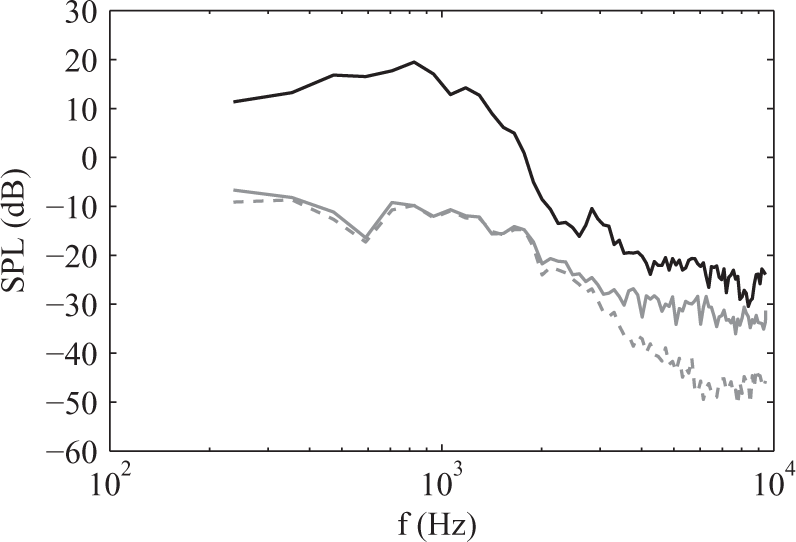$θ = π / 2$ : Total (black line), incident (gray solid line), and incident with quadrupoles only around the trailing edge (gray dashed line).

By contrast, as shown in Figure 6, the radiation in the chord-wise direction is dominated by the incident field across almost all the frequency range, while the scattering effect due to the airfoil wall seems to have only a small effect in general. Both the quadrupoles around the trailing edge and away from these region contribute to the incident quadrupole field.

Figure 6.

Far-field radiation at θ = 0: Total (black solid line), incident (gray solid line), and incident with quadrupoles only around the trailing edge (gray dashed line).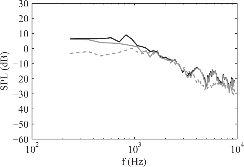

It is worth noting that at high frequencies, the computed acoustic levels at angle θ = 0 (mainly due to the incident field) are higher than those at angle $θ = π / 2$ , which are mainly due to the scattering. This would indicate that at those frequencies the sources are not compact enough to consider Curle’s dipoles as the dominant sources of sound.

As expected, the evolution of the directivity with the frequency follows the typical pattern for trailing-edge problems for a large frequency range, especially at low frequencies. This can be observed in Figure 7. The scattered part of the acoustic field displays an increased number of lobes as the Helmholtz number based on the chord length increases. For the highest frequency shown in the figure (kc = 7.08), the incident quadrupole radiation is already quite large, and it needs to be subtracted to the total field to observe the multilobe pattern.

Figure 7.

Directivity plots of the pressure amplitude at distance 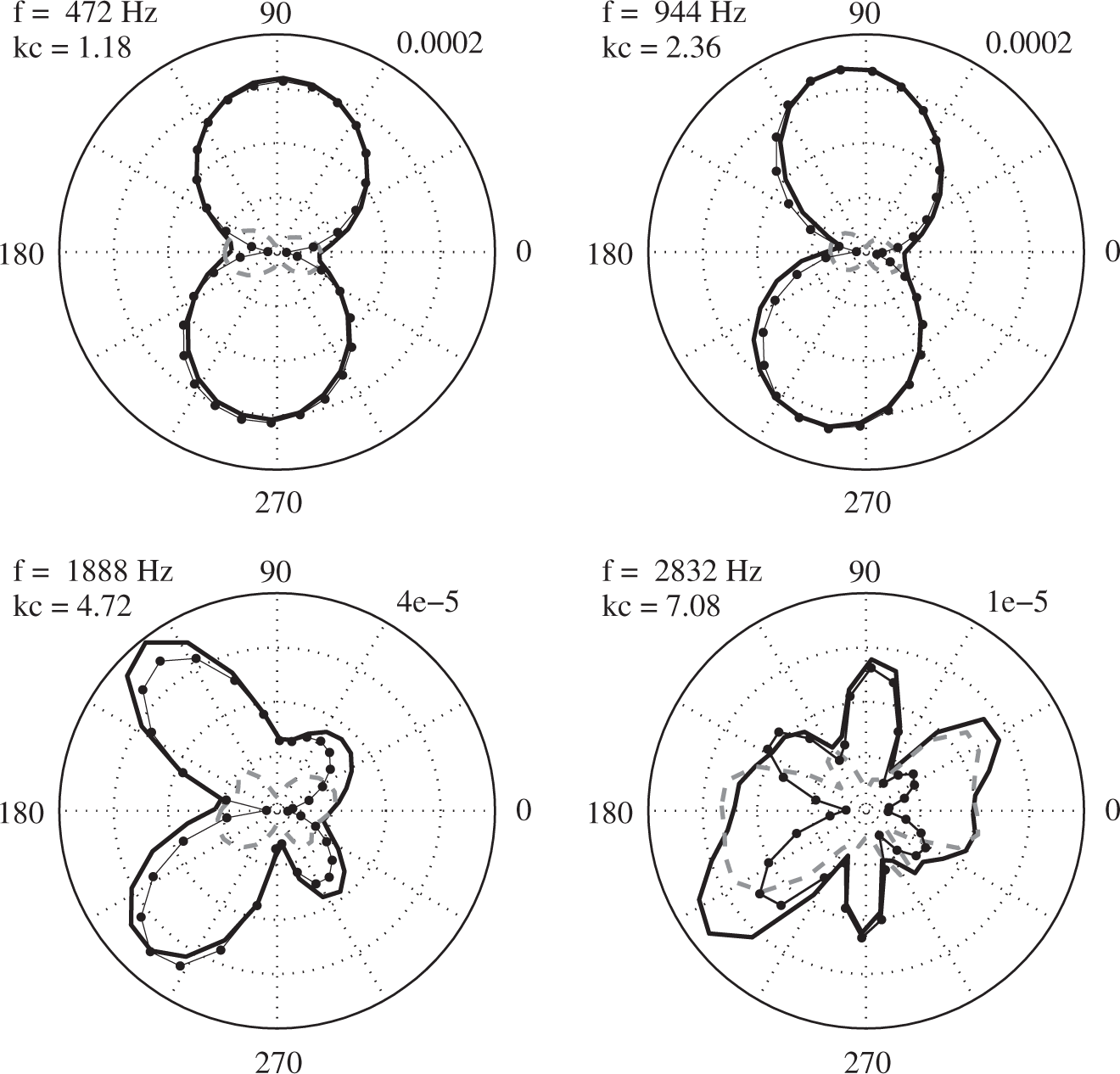$r_{L} = 2 m$ , obtained through the FE computations: total field (solid line), scattered field (line with symbols •), and incident field (gray dashed line). FE: finite element.

Results based on dipole sources

In this section, the results obtained through the FE computations with quadrupole sources are compared to those of the FE computations with dipole sources as BCs. Figure 8 shows results at $θ = π / 2$ . The agreement between the computations with quadrupoles and the computations with dipoles as BCs is good in spite of some deviations at high frequencies, for which the sources are less compact and the approach becomes less accurate.

Figure 8.

Far-field radiation at $θ = π / 2$ : FE computation based on quadrupoles (black solid line), FE computation based on dipoles as BC (black dash-dot line), and Curle’s solution (gray dashed line). BC: boundary condition; FE: finite element.

When comparing with Curle’s solution, the FE results based on dipoles as Neumann BCs prove to overcome some of the limitations due to the use of incompressible pressure data. Indeed, Curle’s solution shows large deviations with respect to the quadrupole solution at high frequencies and fails to reproduce the sharp decrease in amplitude at around 1800 Hz (kc = 4.5). This is due to the fact that Curle’s analogy fails to reproduce the correct physical behavior when it is based on incompressible pressure data defined on a noncompact geometry.

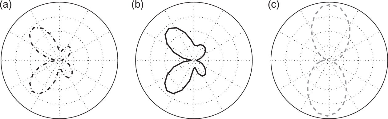
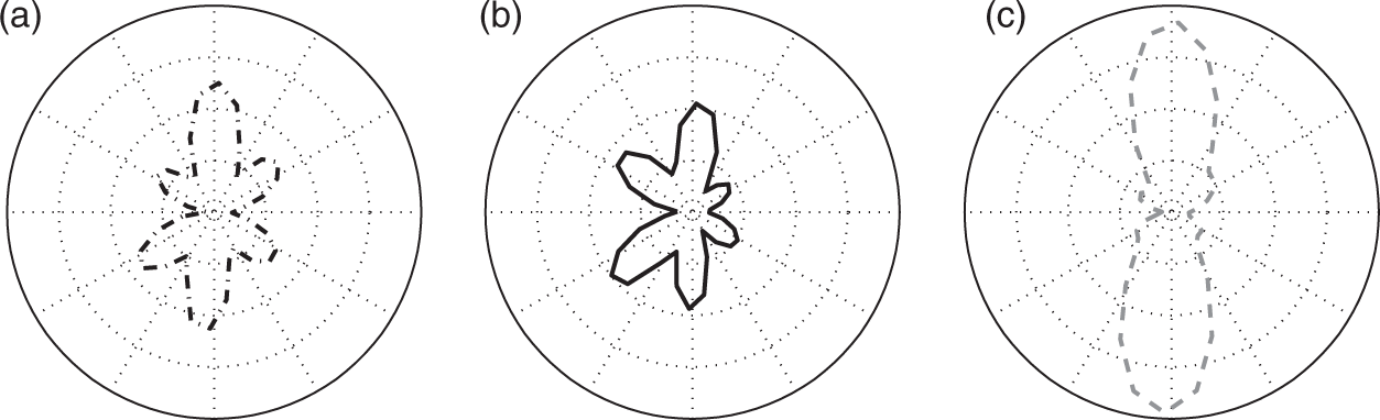
This effect can be seen in more detail in Figures 9 to 11, which show directivity plots of the solution obtained with Curle’s analogy and with the FE computations with quadrupoles (only the scattered field) and dipoles. For low frequencies, for which the Helmholtz number based on the chord length is low, Curle’s analogy presents a similar directivity plot, which shows the behavior of a compact dipole. However, as the Helmholtz number increases, Curle’s solution fails to provide the physical multilobe directivity pattern, which is however obtained with the FE solutions, both with quadrupoles and dipoles. As mentioned before, there is also a frequency limit above which the FE results with dipoles as BCs start to deviate from those with quadrupoles, due to the fact that the incident quadrupole field is not negligible, but this limit is substantially higher than for Curle’s analogy, and, as long as dipole sources (due to the scattering on the wall) are the dominant mechanism of sound production, this approach provides physical and quantitatively meaningful results for the trailing-edge noise scattering.

Figure 9.

Directivity plots of the pressure amplitude at distance $r_{L} = 2 m$ and kc = 1.18: FE results with dipoles (left), FE results for scattered field with quadrupoles (center), Curle’s solution (right). (a) 2e-4, (b) 2e-4, and (c) 2e-4. FE: finite element.

Figure 10.

Directivity plots of the pressure amplitude at distance $r_{L} = 2 m$ and kc = 4.72: FE results with dipoles (left), FE results for scattered field with quadrupoles (center), Curle’s solution (right). (a) 5e-5, (b) 5e-5, and (c) 5e-5. FE: finite element.

Figure 11.

Directivity plots of the pressure amplitude at distance $r_{L} = 2 m$ and kc = 7.08: FE results with dipoles (left), FE results for scattered field with quadrupoles (center), Curle’s solution (right). (a) 1.25e-5, (b) 1.25e-5, and (c) 1.25e-5. FE: finite element.

Conclusions

A numerical study of the self-noise of a CD airfoil has been presented. The numerical approach is based on the acoustic analogy with sources obtained from incompressible LES results. Results of FE computations based on both quadrupole sources, as defined by Lighthill’s analogy, and dipole sources, as defined by Curle’s analogy, have been compared to experimental results and to results obtained with a half-plane GF.

The approach based on the half-plane GF is less computationally expensive than full computations of the acoustic boundary value problem. Moreover, when comparing the results with those obtained with FE computations with sources only around the trailing edge, it can be seen that they are in fair agreement for most of the frequencies of interest. However, at high frequencies, when noncompactness effects increase and other mechanisms of sound production start competing with the trailing-edge scattering, some significant deviations are observed.

Solving the acoustic problem numerically allows tackling arbitrary geometries and does not require prior knowledge of the dominant mechanisms of sound production of a given problem. Indeed, the FE results for this case suggest that, although for a substantial frequency range the problem can be considered as a classical trailing-edge noise problem where scattering effects (dipole sources) dominate over free quadrupole noise, other contributions (free quadrupole noise, scattering of sources closer to the leading edge of the airfoil) start to be considerable as the frequency increases and the source region becomes less compact from an acoustic point of view. The influence at high frequency of a secondary source of sound close to the leading edge (near the flow reattachment point) has been reported in Sanjosé et al.²⁸

It is worth noting that the contribution of the subgrid turbulent scales to the sound production has been neglected in all the computations, and only the effect of the scales resolved by the LES has been included in the quadrupole source models. This assumption is reasonable for this case, at least for the frequencies and radiation directions where the problem is dominated by the scattering by the airfoil wall, including its trailing edge. Nevertheless, for higher frequencies, and especially in the radiation directions where the scattered field is negligible, it is unclear whether the error introduced by this approximation is negligible. This question is beyond the scope of this paper and should be addressed by future research.

The use of aerodynamic surface pressure to define the sources has been investigated too. When the pressure corresponds to an incompressible flow description, it does not satisfy the correct acoustic BCs on the airfoil wall, and Curle’s solution fails to capture the correct physics of the problem. Nevertheless, more accurate results can be obtained if Curle’s dipoles are used to define an intermediate BC for the acoustic boundary value problem. The results presented here confirm that computations purely based on dipoles treated this way succeed in capturing the physics of the acoustic scattering problem. This approach remains accurate as long as the sources are acoustically compact, and, therefore, dipole sources are dominant.

Footnotes

Declaration of conflicting interests

The author(s) declared no potential conflicts of interest with respect to the research, authorship, and/or publication of this article.

Funding

The author(s) received no financial support for the research, authorship, and/or publication of this article.

Appendix 1: Numerical sensitivity study for the FE computations

References

Caro S and Moreau S. Aeroacoustic modeling of low pressure axial flow fans. In: Sixth AIAA/CEAS aeroacoustics conference, Lahaina, Hawaai, 12–14 June 2000. AIAA-2000-22094.

Glegg

SAL

Baxter

Glendinning

. The prediction of broadband noise from wind turbines. J Sound Vib 1987; 118: 217–239.

Hubbard

Shepherd

. Aeroacoustics of large wind turbines. J Acous Soc Am 1991; 89: 2495–2508.

Pérennès S and Roger M. Aerodynamic noise of a two-dimensional wing with high-lift devices. In: Fourth AIAA/CEAS aeroacoustics conference, Toulouse, 2–4 June 1998. AIAA-1998-2338.

Singer

Lockard

Brentner

. Computational aeroacoustic analysis of slat trailing-edge flow. AIAA J 2000; 38: 1558–1564.

Howe

. A review of the theory of trailing edge noise. J Sound Vib 1978; 61: 437–465.

Ffowcs Williams

Hall

. Aerodynamic sound generation by turbulent flow in the vicinity of a scattering half-plane. J. Fluid Mech 1970; 40: 657–670.

Howe

. Edge-source acoustic green’s function for an airfoil of arbitrary chord, with application to trailing-edge noise. Q J Mech Appl Math 2001; 54: 139–155.

Moreau

Roger

. Back-Scattering correction and further extensions of Amiet’s trailing-edge noise model. Part I: theory. J Sound Vib 2009; 286: 477–506.

10.

Moreau

Roger

. Back-scattering correction and further extensions of Amiet’s trailing-edge noise model. Part II: application. J Sound Vib 2009; 323: 397–425.

11.

Amiet

. Noise due to turbulent flow past a trailing edge. J Sound Vib 1976; 47: 387–393.

12.

Manoha

Troff

Sagaut

. Trailing-edge noise prediction using large-eddy simulation and acoustic analogy. AIAA J 2000; 38: 575–583.

13.

Wang

Moin

. Computation of trailing-edge flow and noise using large-eddy simulation. AIAA J 2000; 38: 2201–2209.

14.

Singer

Brentner

Lockard

. Simulation of acoustic scattering from a trailing edge. J Sound Vib 2000; 230: 541–560.

15.

Oberai

Roknaldin

Hughes

TJR

. Computation of trailing-edge noise due to turbulent flow over an airfoil. AIAA J 2002; 40: 2206–2206.

16.

Lighthill

. On sound generated aerodynamically. I. General theory. Proc R Soc 1952; 211: 564–587.

17.

Khalighi Y. Computational aeroacoustics of complex flows at low Mach number. PhD thesis, Stanford University, 2010.

18.

Curle

. The influence of solid boundaries upon aerodynamic sound. Proc R Soc 1955; 231: 505–514.

19.

Ffowcs Williams

Hawkings

. Sound generated by turbulence and surfaces in arbitrary motion. Phil Trans R Soc 1969; A264: 321–342.

20.

Schram C, Anthoine J and Hirschberg A. Calculation of sound scattering using Curle’s analogy for non-compact bodies. In: Proceedings of the 11th AIAA/CEAS aeroacoustics conference and exhibit, Monterey, California, 23–25 May 2005. AIAA-2005-2836.

21.

Schram

. A boundary element extension of curle’s analogy for non-compact geometries at low-Mach numbers. J Sound Vib 2009; 322: 211–232.

22.

Martínez-Lera

Schram

Bériot

. An approach to aerodynamic sound prediction based on incompressible-flow pressure. J Sound Vib 2014; 333: 132–143.

23.

Moreau

Neal

Foss

. Hot-wire measurements around a controlled diffusion airfoil in an open-jet anechoic wind tunnel. J Fluids Eng 2006; 128: 699–706.

24.

Moreau

Roger

. Effect of airfoil aerodynamic loading on trailing-edge noise sources. AIAA J 2005; 43: 41–52.

25.

Moreau S, Neal D, Khalighi Y, et al. Validation of unstructured-mesh les of the trailing-edge flow and noise of a controlled-diffusion airfoil. In: Proceedings of the Summer Program 2006. Centre for Turbulence Research, Stanford University/NASA Ames, 2006.

26.

Wang

Moreau

Iaccarino

. LES prediction of wall-pressure fluctuations and noise of a low-speed airfoil. Int J Aeroacoust 2009; 8: 177–198.

27.

Christophe J, Moreau S, Hamman CW, et al. Uncertainty quantification for the trailing-edge noise of a controlled-diffusion airfoil. In: Proceedings of the Summer Program 2010. Centre for Turbulence Research, Stanford University/NASA Ames, 2010.

28.

Sanjosé M, Moreau S, Kim MS, et al. Direct self-noise simulation of the installed controlled diffusion airfoil. In: Seventeenth AIAA/CEAS aeroacoustics conference, Portland, Oregon, 5–8 June 2011. AIAA-2011-2716.

29.

Moreau

Henner

Iaccarino

. Analysis of flow conditions in freejet experiments for studying airfoil self-noise. AIAA J 2003; 41: 1895–1905.

30.

Christophe J, Moreau S, Schram C, et al. Trailing edge noise prediction of a controlled-diffusion airfoil. In preparation, 2015.

31.

Christophe J and Moreau S. LES of the trailing-edge flow and noise of a controlled-diffusion airfoil at high angle of attack. In: Proceedings of the Summer Program 2008. Centre for Turbulence Research, Stanford University/NASA Ames, 2008.

32.

Winkler J and Moreau S. LES of the trailing-edge flow and noise of a NACA6512-63 airfoil at zero angle of attack. In: Proceedings of the Summer Program 2008. Centre for Turbulence Research, Stanford University/NASA Ames, 2008.

33.

Siemens Industry Software NV, Leuven, Belgium. LMS Virtual. Lab 13.1, User’s Manual, 2014.

34.

Colonius

. Modeling artificial boundary conditions for compressible flow. Annu Rev Fluid Mech 2004; 36: 315–345.

35.

Bériot H and Tournour M. On the locally-conformal perfectly-matched layer implementation for Helmholtz equation. In: Mace BR, Ferguson NS, Rustighi E (eds) Noise and Vibration: Emerging Methods (NOVEM) 2009, Oxford, 5–8 April 2009.

36.

Vansant K, Hallez R, Bériot H, et al. Simulating acoustic engine performance over a broad frequency range. In: SAE International, Detroit, Michigan, 12–14 April 2011. Technical paper 2011-26-0019.

37.

Bériot H, Prinn A and Gabard G. On the performance of high-order FEM for solving large-scale industrial acoustic problems. In: Proceedings of the 20th International Congress on Sound and Vibration, Bangkok, Thailand, 7–11 July 2013. IIAV.

38.

Wang

Lele

Moin

. Computation of quadrupole noise using acoustic analogy. AIAA J 1996; 34: 2247–2254.