



Abstract
The change of helicopter rotor broadband noise due to different surface roughness during ice accretion is investigated. Comprehensive rotor broadband noise measurements are carried out on rotor blades with different roughness sizes and rotation speeds in two facilities: the Adverse Environment Rotor Test Stand facility at The Pennsylvania State University, and the University of Maryland Acoustic Chamber. In both facilities, the measured high-frequency broadband noise increases significantly with increasing surface roughness height. Rotor broadband noise source identification is conducted and the broadband noise related to ice accretion is thought to be turbulent boundary layer-trailing edge noise. Theory suggests turbulent boundary layer-trailing edge noise scales with Mach number to the fifth power, which is also observed in the experimental data confirming that the dominant broadband noise mechanism during ice accretion is trailing edge noise. A correlation between the ice-induced surface roughness and the broadband noise level is developed. The correlation is strong, which can be used as an ice accretion early detection tool for helicopters, as well as to quantify the ice-induced roughness at the early stage of rotor ice accretion. The trailing edge noise theories developed by Ffowcs Williams and Hall, and Howe both identify two important parameters: boundary layer thickness and turbulence intensity. Numerical studies of two-dimensional airfoils with different ice-induced surface roughness heights are conducted to investigate the extent that surface roughness impacts the boundary layer thickness and turbulence intensity (and ultimately the turbulent boundary layer-trailing edge noise). The results show that boundary layer thickness and turbulence intensity at the trailing edge increase with the increased roughness height. Using Howe’s trailing edge noise model, the increased sound pressure level of the trailing edge noise due to the increased displacement thickness and normalized integrated turbulence intensity are 6.2 and 1.6 dB for large and small accreted ice roughness heights, respectively. The estimated increased sound pressure level values agree reasonably well with the experimental results, which are 5.8 and 2.6 dB for large and small roughness height, respectively.
Keywords
Introduction
Compared to fixed-wing aircraft, helicopters are more likely to be affected by icing problems due to their comprehensive mission requirements. However, helicopter rotor ice accretion is not well understood due to complexities in the 3D environment with inherent unsteady flow. To address helicopter icing issues, a helicopter icing physics, modeling, and detection project was undertaken at the Penn State Vertical Lift Research Center of Excellence. The main objective of this project is to gain a fundamental understanding of ice accretion on helicopter rotor blades. Three research groups, involving experiments and computational fluid dynamics (CFDs) and acoustics, worked together to achieve this goal.
This paper presents some results from the acoustic task. The aim of the acoustic task was to investigate the rotor noise during ice accretion and determine if different rotor noise source mechanisms, for example, thickness noise, steady loading noise, and broadband noise, can be used to detect the formation and location of accreted ice, especially at the early stage of ice accretion when the “ice” essentially changes the surface roughness of the lifting surface. Previous studies1–3 show that rotor discrete frequency (thickness and steady loading noise) noise is changed noticeably during ice accretion, but the change is too small to be used in icing detection. The focus of this paper is to summarize and highlight the surface roughness effect, especially the ice-induced surface roughness, on rotor broadband noise in the previous studies.1–3
Generally, helicopter rotor broadband noise can be divided into the following sources: (1) turbulence ingestion noise; (2) blade wake interaction (BWI) noise; and (3) blade self-noise, which includes five individual source mechanisms: turbulent boundary layer-trailing edge (TBL-TE) noise, separation-stall noise, laminar boundary layer-vortex shedding (LBL-VS) noise, trailing edge bluntness-vortex shedding noise, and tip vortex formation noise, as described by Brooks et al. 4
TBL-TE noise is produced at high Reynolds numbers, when turbulence generated from the turbulent boundary layer passes over the sharp trailing edge. Devenport et al.
5
and Glegg and Devenport
6
demonstrated that surface pressure fluctuations directly relate to far-field noise generation. They also presented how the far-field noise generated by a boundary layer over a rough surface depends on the surface pressure wavenumber spectrum and the roughness geometry. Thus, the ice-induced surface roughness and the resulting turbulence are expected to primarily affect the TBL-TE noise. A comprehensive experimental study of airfoil self-noise and its prediction was done by Brooks et al.
4
and Brooks and Marcolini.
7
In their study, a boundary layer tripping technique was applied to ensure a fully developed turbulent boundary layer at the trailing edge when investigating the TBL-TE noise. Such a tripping technique (applying a strip on the airfoil from the leading edge to 20% chord with a random distribution of grit) is very similar to the ice-accreted roughness (actual or simulated) considered in the present work. However, the effect of the grit size on TBL-TE noise was not discussed, as only one grit size was used for the tripping of most of the airfoils. Other investigations5,6,8 have studied the noise of roughened walls or flat plates,5,6,8 which do not have a sharp trailing edge. Noise from the roughened wall is due to scattering of the turbulence into sound by roughness elements rather than by the trailing edge. So the TBL-TE noise source mechanism is thought to be different than that from a roughened wall. The present work aims to:
Show comprehensive rotor broadband noise measurement results due to surface roughness during ice accretion with different blade sizes, roughness sizes, and rotor rotation speeds. Correlate the rotor broadband noise to the ice-induced surface roughness height and to develop a tool to predict the roughness height from rotor noise based on such a correlation. Propose that the broadband noise source due to roughness is TBL-TE noise, demonstrate that the noise follows the proper scaling law for this noise source, and qualitatively explain why higher roughness height tends to give a higher noise level.
The following sections introduce the experiment setup and results. Comprehensive rotor broadband noise measurements due to surface roughness during ice accretion have been conducted in two facilities: the Adverse Environment Rotor Test Stand (AERTS) facility at The Pennsylvania State University, and the University of Maryland Acoustic Chamber (UMAC). Then, emphasis shifts to explain why rotor broadband noise increases with surface roughness height at high frequencies. In “Experimental investigation” section, a theoretical analysis of trailing edge noise is conducted. Two parameters, boundary layer thickness and turbulence intensity at the trailing edge are discussed. These are considered to be the key factors that cause the broadband noise increase based on the trailing edge noise theory of Ffowcs Williams and Hall 9 and Howe. 10 Then a correlation between the surface roughness height and the broadband noise level has been developed. “Numerical investigation” section describes a numerical investigation of the change of the boundary layer thickness and the turbulence intensity of a 2D airfoil due to different ice-induced surface roughness. Some conclusions are drawn in the final section.
Experiment setup
AERTS test
Proof-of-concept measurements have been performed in the AERTS facility at Penn State to explore the effect of different surface roughness heights on rotor broadband noise. Figure 1 shows the facility with two NACA 0012 test blades (“paddle blades”). The facility can accommodate test blades with dimensions up to 0.813 m (31 in.) chord and 3 m (10 ft) diameter. The test stand is located inside a cold chamber that is capable of maintaining constant temperatures ranging from 0 to −25°C during the tests. A detailed description of the AERTS facility can be found in Han and Palacios. 11 One concern is the acoustic environment in the AERTS facility. The octagonal sidewalls (hard walls), the flat ceiling (not shown in Figure 1), as well as the complicated rotor stand shape under the rotor plane prevent the facility from being an ideal acoustic test chamber. The unfavorable acoustic situation in the AERTS facility is considered to be acceptable for the current proof-of-concept testing and not unlike the situation on an aircraft.

AERTS facility with test blades mounted (See colour version of this figure online).
A 1/4″ microphone (PCB 130E21) is located above the rotor plane, as shown in Figure 3, in a region where broadband noise is expected to be significant and away from the complicated cover shape of the rotor test stand. It is also placed relatively far (0.4 m) from the sidewall to avoid a strong acoustic reflection. The distance from the microphone to the rotor plane is 0.46 m, and its distance to the rotor shaft axis is 1.26 m. The microphone location for all the broadband measurements is fixed at this position.
The test “paddle blade” geometry used in this study is shown in Figure 2. The blade radius is 1.372 m (54 in.). The outboard part is the ice shape monitoring area, labeled as the “paddle blade.” The chord of the “paddle blade” section is 53.34 cm (21 in.), which is designed to have the same profile (NACA 0012) and chord length as an airfoil used in several icing experiments at the NASA Icing Research Tunnel.12,13

AERTS "paddle blade" (See colour version of this figure online).
For the first tests, rotor broadband noise measurements for blades with simulated roughness were conducted. Sandpaper with different grit sizes was applied to the leading edge of the “paddle blade” to represent the surface roughness during the early stage of the ice accretion. The advantage of sandpaper over accreted ice is that the roughness element size of the sandpaper is provided by the vendor. The “paddle blades” are covered by sandpaper at the leading edge as can be seen in Figure 3(a). The chordwise extent of the sandpaper is 10% of the chord, which is representative of the extent of ice-induced surface roughness. Sandpaper with different grit sizes was used to represent different surface roughness heights corresponding to different time intervals of ice accretion. The sandpaper grit sizes are shown in Table 1. The rotation speeds used for the broadband noise measurements were 200, 300, and 400 r/min, which corresponds to tip speeds of 29.7, 44.6, and 59.4 m/s, respectively.

AERTS microphone location (See colour version of this figure online).
Sandpaper grit size table.

After the broadband noise measurements with simulated roughness, measurements of the broadband noise generated by accreted ice were performed. To protect the microphone from the icing cloud, the microphone was removed from the chamber when generating the ice, and then remounted at the same location as it was during the sandpaper test (above the rotor) after the ice has been accreted on the “paddle blades.” Finally, the broadband noise was measured in the cold environment. The r/min was set to 450 for the ice accretion testing (blade tip speeds of 66.7 m/s). The ice accretion conditions used to generate different ice surface roughness are listed in Table 2. Notice that the maximum icing time for all cases was 2 min because the focus is placed on the early stage of the ice accretion. Longer icing time would result in accumulation of large amounts of ice, which is no longer representative of ice-induced roughness. The typical ice-induced surface roughness shapes, as seen looking toward the end of the blade toward the blade tip, are shown in Figure 4. In the figure, case 12 (left) is one of the roughest shapes among all cases evaluated and case 15 (right) is one of the smoothest.
Icing conditions with different ice-induced surface roughness.


Ice-induced surface roughness at the tip of the “paddle blade” test section. (a) Case 12 and (b) case 15 (See colour version of this figure online).
UMAC test
Another set of broadband noise measurements due to surface roughness has been conducted in the UMAC. Some key differences in the testing at UMAC include: (1) it is an anechoic chamber, (2) the rotor test stand is able to operate at a higher rotational speed (up to a hover tip Mach number of 0.7—typical of full-scale helicopters), and (3) the blade chord size is smaller and the surface roughness material used to simulate accreted ice is different from that used in the AERTS test. Testing with different chord size, roughness height, and different rotor r/min makes it possible to investigate the correlation between broadband noise frequency content and these parameters. The disadvantage of testing in UMAC is that the rotor broadband noise resulting from real ice-induced surface roughness cannot be tested—only representative surface roughness can be used.
The chamber is an octagonal 20 ft by 20 ft wide, 30 ft tall acoustically treated facility. Four different blade surface roughness sizes as well as the clean blades are used to investigate different roughness height effects on rotor broadband noise. For each blade set, broadband noise is measured at every 10th of tip Mach number, from 0.1 to 0.7, by a single microphone.
Figure 5 shows the rotor system of the UMAC, which is a single bladed, counterweighted, rigid rotor with a 2° downward collective pitch. This produces a very small amount of downward thrust in order to push the rotor wake above the rotor plane and provide as clean an acoustic environment as possible. (Note: In the UMAC test the rotor thrust is directed downward and the rotor wake goes upward from the rotor.) More details about the facility can be found in Sim 14 and Koushik 15 Figure 6 shows the rotor blade used in this test, which is a rectangular, untwisted blade with NACA 0012 airfoil sections. The chord and radius are 0.0762 m (3 in.) and 0.9398 m (37 in.), respectively.

UMAC rotor system (See colour version of this figure online).

UMAC NACA0012 rectangular blade (with hub and the counter weight) (See colour version of this figure online).
Four different surface roughness sizes were applied in the test to represent different surface roughness heights corresponding to different time intervals in the real ice accretion case. Due to the relatively small size of the blade chord, sandpaper could not be applied on the clean blade to represent the ice-induced surface roughness as was done in the AERTS test. The thickness of the sandpaper layer itself (rather than the grit on the sandpaper) is significant compared to the blade thickness and there was concern that the extra thickness could have an impact on boundary layer characteristics, as well as the trailing edge turbulence, which would finally influence the rotor broadband noise. Consequently, two alternative roughness application techniques (roughness elements only) are used: commercial glass beads or sugar crystals were bonded to the leading edge with lacquer for the larger roughness sizes, and commercial texture paint was used for the smaller roughness heights. (For this test KRYLON texture paints—SILVER and OBSIDIAN—were used.) Figure 7 shows the sugar crystals, glass beads, and texture paint on the blade. Both glass beads/sugar crystals and texture paints are applied on the leading edge of the clean blade (both upper and lower surfaces).

UMAC rotor blade with different surface roughness applied. (a) Sugar crystals (1.02 mm), (b) glass beads (0.50 mm), (c) texture paint OBSIDIAN (0.20 mm), and (d) texture paint SILVER (0.12 mm) (See colour version of this figure online).
A roughness height characterization was carried out because the roughness size of the sugar crystals and the texture paint was not known. Detailed characterization process can be found in Cheng et al. 2 The arithmetic averages of measured peak-to-valley roughness heights for the sugar crystal and the texture paints (OBSIDIAN and SILVER) are 1.02, 0.50, 0.20, and 0.12 mm, respectively.
One 1/4″ microphone (PCB 378C01) is used in this test. It has a high frequency capability up to 100 kHz. High-frequency performance of the microphone is expected to be critical in these tests. The manner in which the broadband noise frequency content changes with turbulence scale, blade size, and rotor rotational speed was not known before the test. However, the relationship between the broadband noise frequency range and the rotational speed (tip Mach number) in the AERTS test showed that rotor broadband noise due to different blade surface roughness tends to separate from each other at frequencies higher than 10 kHz when the rotational speed increases. Consequently, for high rotational speed tests in UMAC, a microphone with a frequency range up to 100 kHz (compared to the 24 kHz microphone used in AERTS test) is used and the measurement results show that this frequency range is sufficient for the current tests. The microphone is located out of the rotor plane with a distance 0.98 R2 (R2 = 0.9398 m) away from the hub center and a 20° elevation angle. The nondimensional microphone location is set to be the same as the position used in the AERTS test (nondimensionalized by rotor radius) for comparison purposes.
Experiment results
AERTS test
A sample rate of 48,000 samples/s was used in the data acquisition of the test in AERTS, which corresponds to 24 kHz. Acoustic pressure data were recorded for 4 s for each broadband noise measurement. The measured time-domain broadband results data were analyzed and presented as the pressure spectra on a linear frequency scale. An averaging process was applied to each sound pressure level (SPL) spectrum to show a smoother and clearer SPL trend. The segment length of each data time series used for averaging was 300 data points (0.00625 s), with 50% overlap (150 data points) with respect to the adjacent segment. A Hanning window was applied to each time segment. The averaged SPLs for the cases with sandpapers of different surface roughness heights and the clean blades for the 400 r/min rotational speed are first shown in Figure 8. The background (BG) noise is also shown. This is the noise from the rotating rotor stand without any blades. A clear trend can be seen in the frequencies higher than 8 kHz. The rougher surface (higher roughness height) gives a higher SPL value. SPL values from other two rotational speeds—200 and 300 r/min—show same trend, but the results are not shown here.

AERTS test results: SPL from different sandpaper roughness, clean blades, and BG (400 r/min, tip Mach number 0.17). BG: background (See colour version of this figure online).
Figure 9 shows the SPL spectra comparison between clean blades and the two example roughness shapes shown in Figure 4, where the surface roughness was due to actual ice accretion. In the cases shown in Figure 9, the rotational speed was slightly higher, 450 r/min, but the measurements have all the same features as the sandpaper generated roughness (Figure 8). From Figure 9, it is clear that these two different surface roughness cases can be distinguished by looking at the SPL in the high frequencies. For example, case 12 (large surface roughness) is approximately 2 or 3 dB noisier than case 15 (small surface roughness) at frequencies larger than 15 kHz, even if the ice roughness elements are not as uniformly distributed as those of the sandpaper. To be clear, SPLs from other ice-induced surface roughness (other cases in Table 2) are not shown.

AERTS test results: SPL from two different ice-induced surface roughnesses and their comparison with that from the clean blades (450 r/min, tip Mach number 0.2) (See colour version of this figure online).
UMAC test
The rotor blades in the UMAC test had considerably smaller chord and the rotation rates were significantly higher. Therefore, the sample rate used during data acquisition for the UMAC test was 200,000 samples/s. Four seconds of acoustic pressure data were recorded for each broadband noise measurement. Again an averaging process is applied to each SPL spectrum in which the segment length of each time series used is 5000 data points (0.025 s), with no overlap. A comprehensive tip Mach number range from 0.1 to 0.7 was covered for the rotor broadband noise measurements. Typical SPL comparisons between roughened blades and the clean blade at tip Mach number equal to 0.4 and 0.6 are shown in Figure 10. A similar trend is obtained that the rougher blade gives a higher SPL at high frequencies (larger than 30 kHz). Notice that for UMAC test the lowest frequency where SPL from different surface roughness can be distinguished from each other occurs at an even higher frequency than the AERTS test (Mach number 0.17), i.e. 30 and 50 kHz (Mach number 0.4 and 0.6) as opposed to 12 kHz. Such an increase in frequency was expected for the UMAC test. The broadband noise frequency content is thought to correlate with rotor rotational speed, as well as the blade size, roughness height, and turbulence scale. However, a more comprehensive acoustic experiment with different blade scales and roughness sizes, as well as detailed 2D wind tunnel flow tests would be needed to investigate such a correlation relationship in detail.
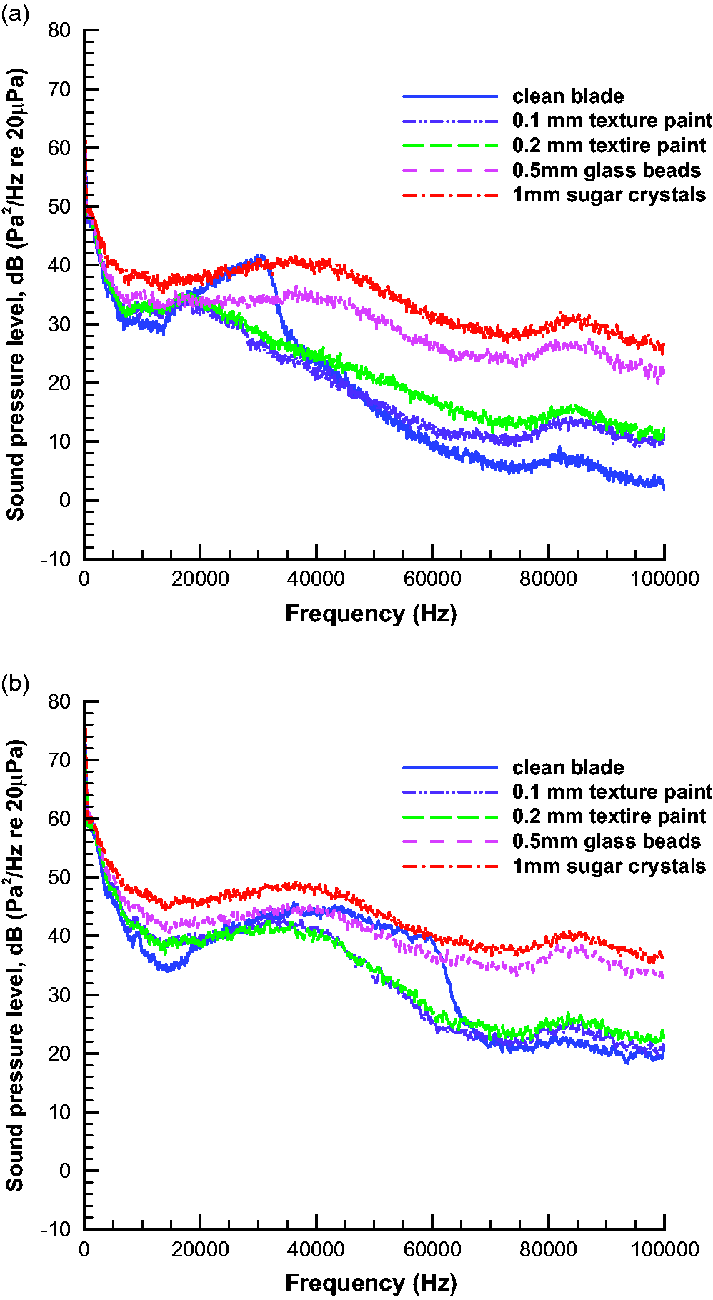
UMAC test results: SPL from four different surface roughnesses and their comparison with that from the clean blade. (a) Tip Mach number = 0.4 and (b) Tip Mach number = 0.6 (See colour version of this figure online).
In Figure 10(a), another interesting feature lies in the SPL from the clean blade, which shows a SPL magnitude “peak” around 30 kHz where the SPL level for the clean blade is higher than that from the roughened blades. This peak is thought to be due to the LBL-VS noise. Similar test results are also reported by Brooks and Marcolini 7 and Peterson and Amiet. 16 As for the LBL-VS noise peak in Figure 10(b), the peak seems to scale to higher frequencies around 60 kHz due to the higher tip Mach number. The reason for this behavior is unknown. It is not thought that the LBL-VS noise mechanism is relevant to the rotor icing problem.
Experimental investigation
Noise source mechanism identification
Helicopter rotor broadband noise sources can be divided into: (1) turbulence ingestion noise, (2) BWI noise, and (3) blade self-noise. Blade self-noise includes five individual source mechanisms: TBL-TE noise, separation-stall noise, LBL-VS noise, trailing edge bluntness-vortex shedding noise, and tip vortex formation noise, as described by Brooks et al. 4 It is critical to identify the noise source mechanism that causes the rotor broadband noise increase due to ice-induced surface roughness from the mechanisms listed above before any physical understanding or explanation can be made.
Helicopter rotor turbulence ingestion noise is caused by the interaction between the distorted atmospheric turbulence and rotor blades. It is obvious that the ice-induced surface roughness on rotor blades would not affect the atmospheric turbulence. So turbulence ingestion noise is not considered in the present work. BWI noise is a broadband noise source due to the interaction of the rotor blades with the turbulent portion of the wakes of previous blades, particularly about tip vortices. 17 It is found primarily in level flight to mild climb conditions and depends, to first order, on the rotor tip-path-plane angle. 17 However, the present experiments in both the AERTS and UMAC facilities are hover tests of lightly loaded rotors with a zero degree tip-path-plane angle. So is not expected that BWI noise will be affected noticeably by ice accretion in these facilities. Another reason that the BWI noise is not considered the primary source mechanism during ice accretion is that BWI noise contributes at relatively low frequency, which is in contrast to the high frequency range where the changes in broadband noise due to ice accretion are observed. As shown in Figure 11, from Brooks and Burley, 17 the measured noise spectra of a model BO-105 helicopter with different tip-path-plane angles (used in their BWI noise investigation), the frequency range over which BWI noise appears is from about 1.5 to 6.5 kHz as indicated. An additional frequency scale is also presented in Figure 11, which corresponds to what an observer would hear for an equivalent full-scale rotor scaling on the blade passage frequency. By performing the same frequency scaling, the frequency ranges (if the BWI noise exists) in AERTS (450 r/min as shown in Figure 9) and UMAC (1370 r/min as shown in Figure 10) should be 0.3–1.4 and 0.5–2.0 kHz, respectively. These are much smaller than the SPL frequency ranges with increased levels caused by the ice-induced surface roughness. The other blade self-noise source mechanisms are less likely to contribute to the broadband noise. Separation-stall noise will not occur because the blades are lightly loaded and clearly not stalled or separated; LBL-VS noise is not expected because the surface roughness ensures the boundary layer is turbulent; trailing edge bluntness-vortex shedding noise can be ruled out because the trailing edges of the airfoils are not blunt; and tip vortex formation noise is not expected to be strong because the blades in the experiments are lightly loaded with very weak tip vortices.
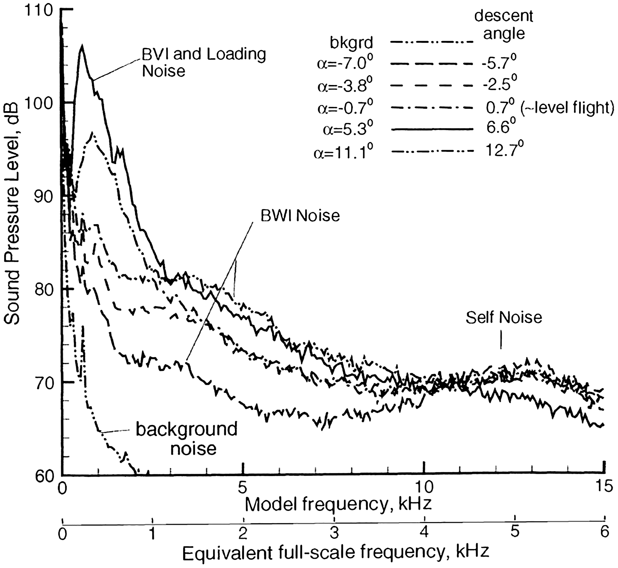
Noise spectra of a model BO-105 helicopter rotor measured in DNW by Brooks and Burley. 17 BWI: blade wake interaction.
Of the different blade self-noise source mechanisms, the TBL-TE noise is the only source that would likely cause the increased rotor broadband noise due to the ice-induced surface roughness. TBL-TE noise is generated when the blade boundary layer turbulence passes over the sharp trailing edge. The ice-induced surface roughness at the leading edge and the resulting turbulence changes are expected primarily to affect the TBL-TE noise. Other self-noise sources will not be addressed in this paper, as they are not thought to be directly relevant to the effects of ice accretion.
Trailing edge noise theory
One of the first analytical solutions of Lighthill’s acoustic analogy for turbulence diffraction about a semi-infinite plane is given by Ffowcs Williams and Hall.
9
They also point out that trailing edge acoustic intensity increases in proportion to the fifth power of the flow velocity. Howe
10
then extended Ffowcs Williams and Hall’s scaling law of a single eddy to all eddies along a plate with a spanwise extent L. Howe’s trailing edge noise scaling law is

Based on the result that trailing edge noise scales with the fifth power of flow velocities, the measured SPL spectra were scaled by Mach number. Only the UMAC test results are scaled here because of the larger range of velocities in the test. Indeed, the motivation of the UMAC test was to check the velocity scaling of the roughness-generated noise. Figure 12 shows the measured SPL of glass beads (0.5 mm) for different tip Mach numbers. SPL results from Mach number 0.1 and 0.2 are not shown because the SPL values are low and they are contaminated by an electrical noise observed during the test. Higher tip Mach numbers result in higher SPLs. Each spectrum curve is separated by at least 4 dB from the next closest curve. SPL spectra from each tip Mach number show the same spectral shape for the entire frequency range: 0–100 kHz. This illustrates the possibility of the velocity scaling. Scaled SPL spectra based on the fifth power of flow velocities (tip Mach numbers) are then shown in Figure 13. It is seen that the spectra collapse well (within 3–4 dB) in the frequency range from 0 to 60 kHz. At the highest frequencies—larger than 60 kHz—the collapse is not as good (within 6–7 dB). Overall, the spectra scaling results confirm that the broadband noise source mechanism related to surface roughness is trailing edge noise. Other velocity scalings were also considered, but they did not collapse the measurements as well as the scaling shown in Figure 13. A detailed spectrum scaling study of TBL-TE noise, as well as the LBL-VS noise can be found in Cheng. 3
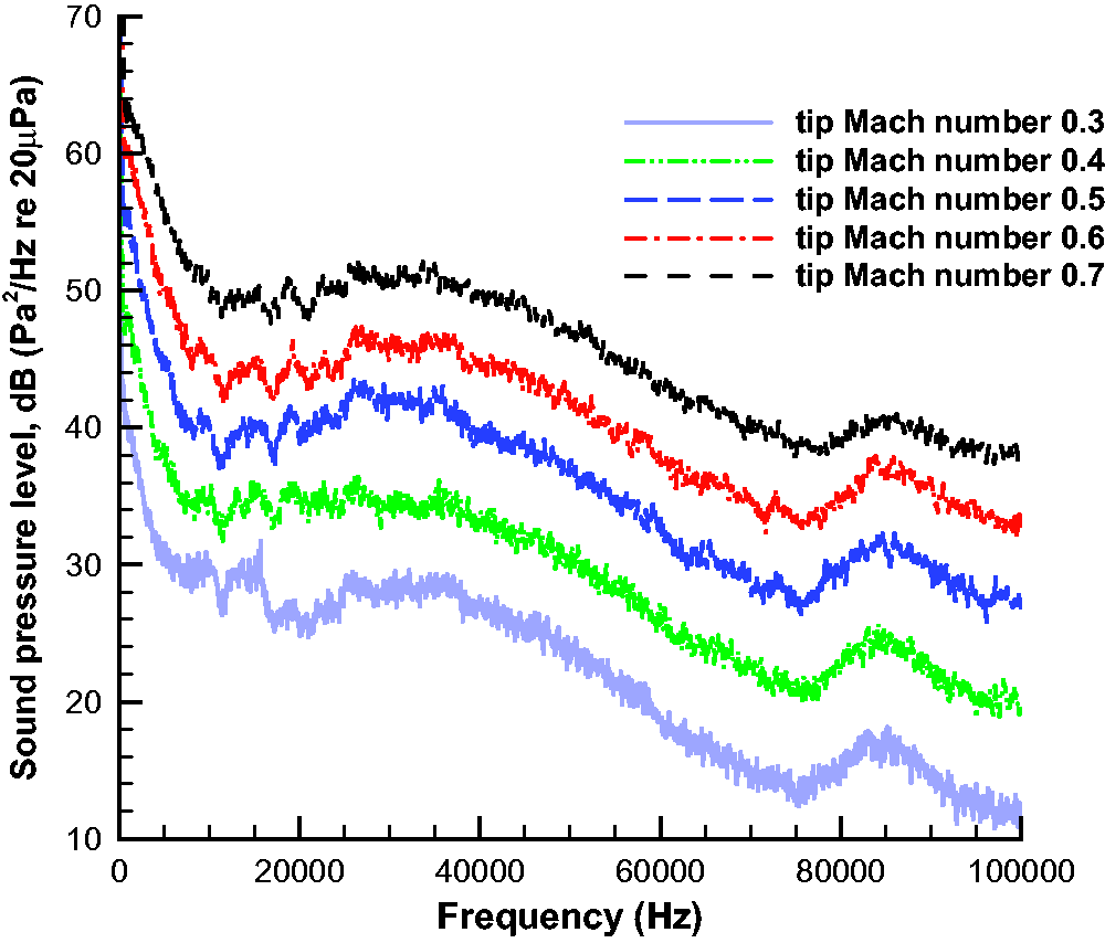
Measured noise spectra of the blade with glass beads at different tip Mach numbers (0.5 mm glass beads not scaled) (See colour version of this figure online).
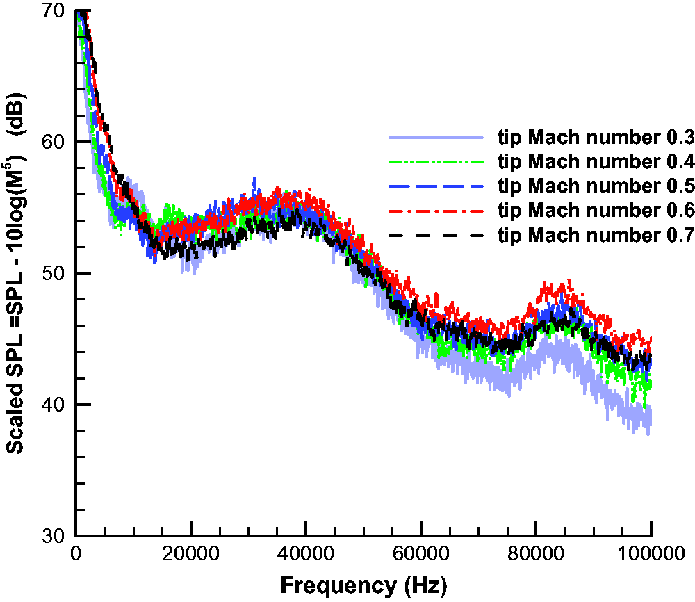
Scaled noise spectra of Figure 14 based on the fifth power law of flow velocities (0.5 mm glass beads scaled on M5). SPL: sound pressure level (See colour version of this figure online).
Correlation between surface roughness height and broadband noise level
1. Ice-induced surface roughness digitization
To correlate the ice surface roughness to the broadband noise, one needs to quantify the ice-induced surface roughness. A specific concern to describe the roughness in the present work is that all the roughnesses used are from the relatively early stage of the ice accretion. As described by Shin, 18 roughness shapes from different icing conditions follow a same initial trend at the beginning of the exposure to the icing cloud as shown in Figure 14.
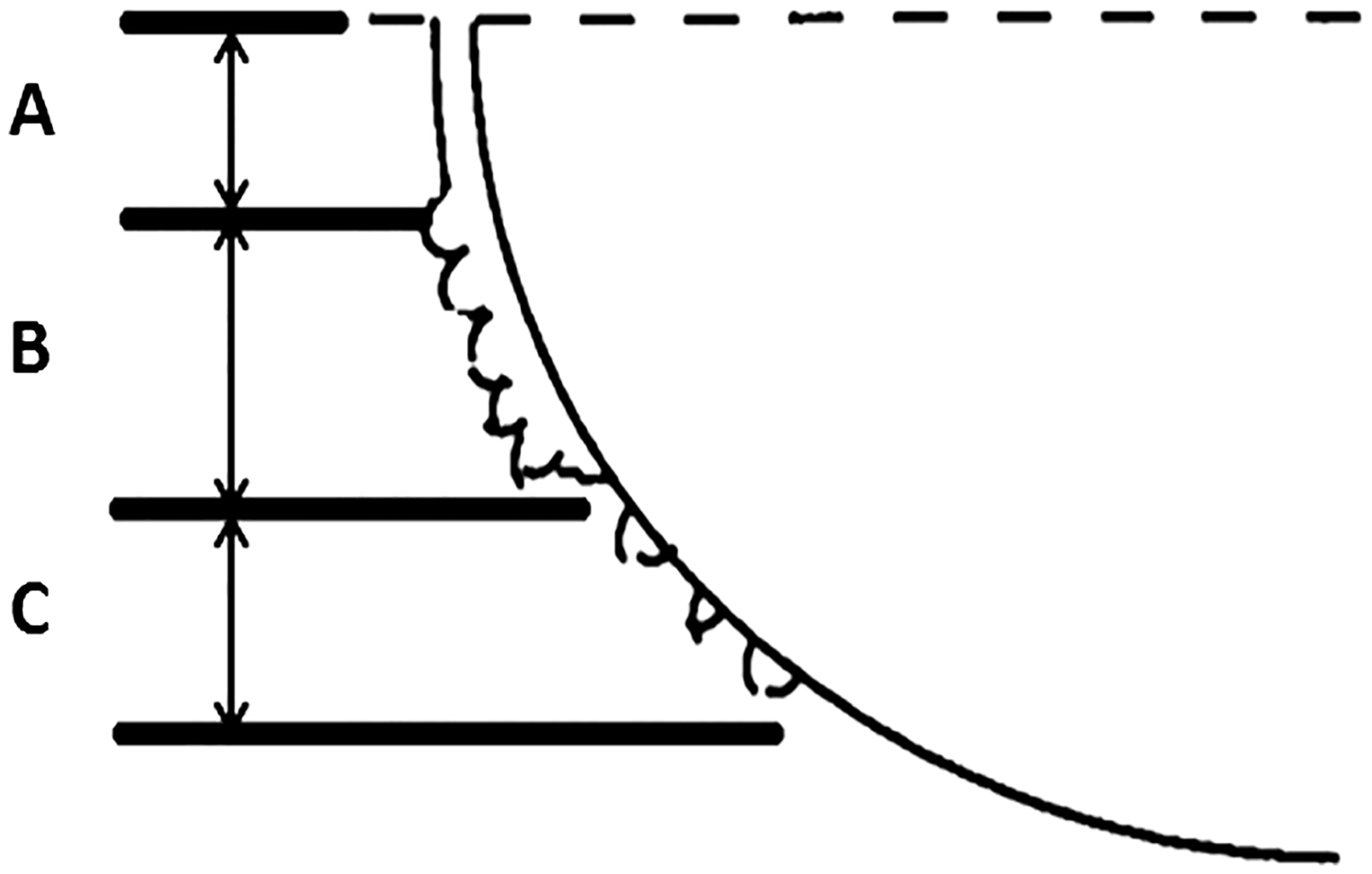
Illustration of ice-induced roughness growth at early stage. 19
Three regions are identified in the initial ice accretion procedure: region A is the smooth zone which is just a smooth layer of ice, region B is the roughness zone in which the roughness develops on an ice substrate that has a fairly uniform thickness, and region C is where some small ice bumps develop at various spots but without the ice substrate. This initial roughness trend is confirmed by the present work as shown in Figure 15. The smooth zone and rough zone can be seen in Figure 15(a), and the ice roughness feature is clearly shown in Figure 15(b). Figure 15 also shows an example of the blade tip roughness digitization process. A small grid attached to end of the blade tip is used as a length reference during digitization. The grid size is 1.88 mm × 1.88 mm and is placed parallel to the airfoil chord line. The GetData Graph Digitizer 20 is used in the roughness digitization process. For each case, the coordinate for digitization is the same, which is defined based on the grid: the origin is located at the left and bottom corner, the x-axis is along the bottom of the grid and the y-axis along the left border as shown in Figure 15(a). Then both the clean airfoil and the roughness boundary are digitized, as shown in Figure 16(a).
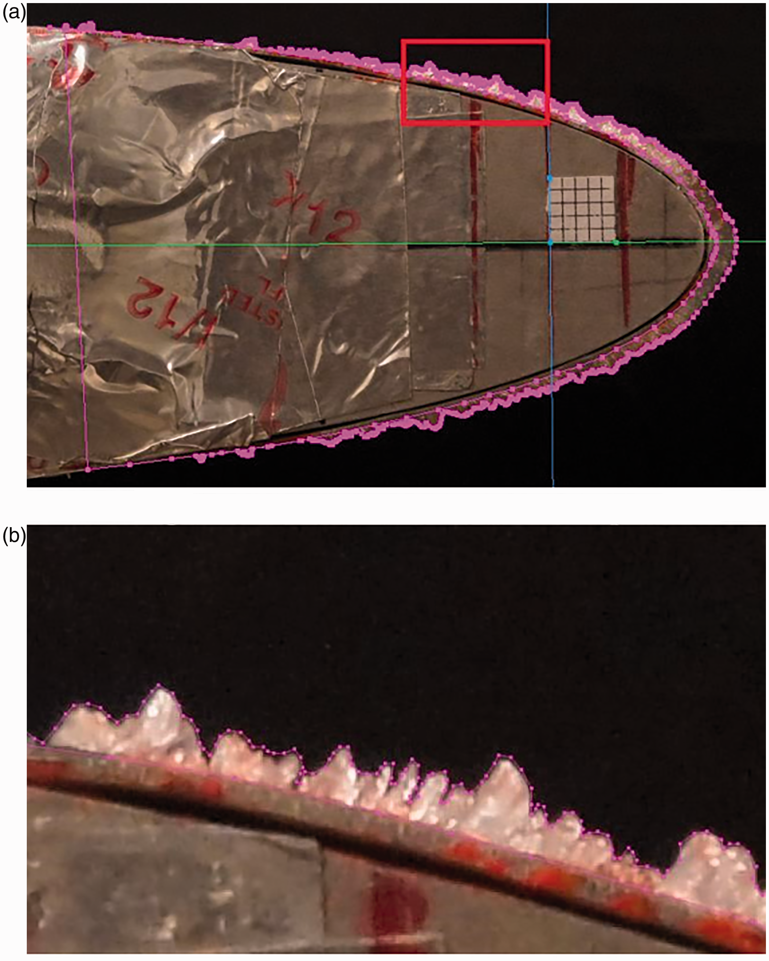
Photo of the surface roughness digitization at the blade tip (case 12). (a) Digitization of both clean and iced profile and (b) close-up of the red region (See colour version of this figure online).
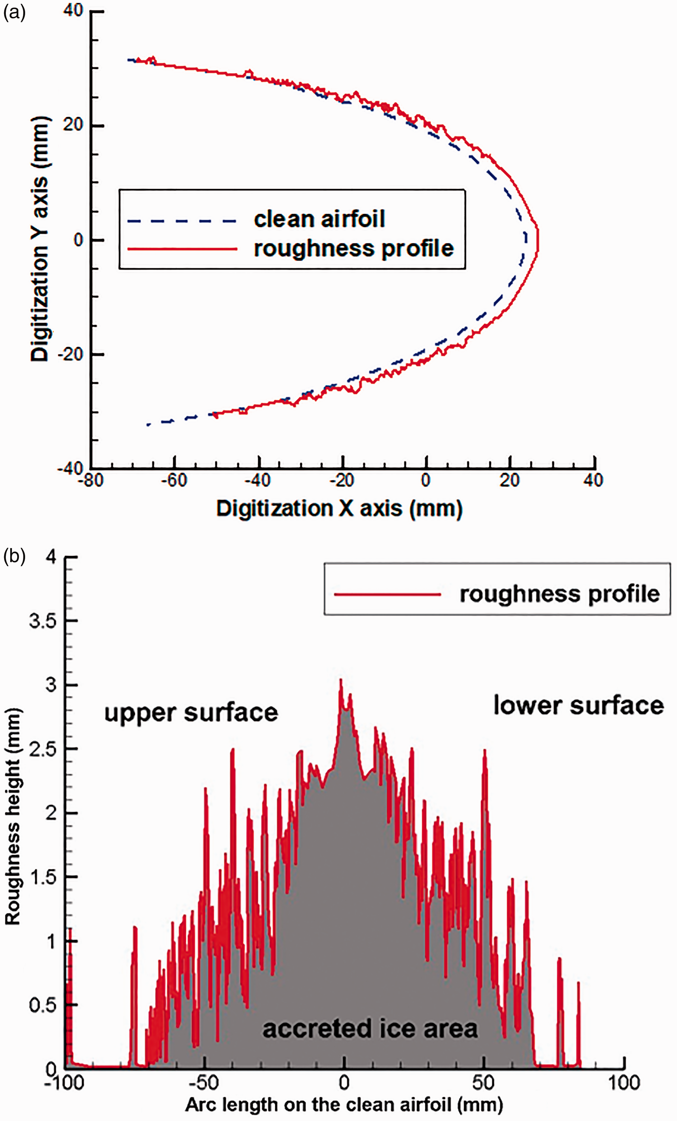
Digitized roughness profile. (a) Original digitized plot and (b) unwrapped along the clean airfoil arc (See colour version of this figure online).
The digitized roughness boundary is also unwrapped along the clean airfoil arc in order to measure the roughness height and the ice area as shown in Figure 16(b), in which the zero arc length value indicates the stagnation point. Digitized points on negative x-axis represent the roughness on the upper surface of the airfoil and those on the positive x-axis represent the roughness on the lower surface.
Figure 17 shows digitized roughness profiles from different icing conditions. For the sake of clarity, not all roughnesses are shown in this figure. For each roughness profile, the three zones are distinguishable. However, the length of the smooth zone and roughness zone is different from case to case, as is the roughness height.
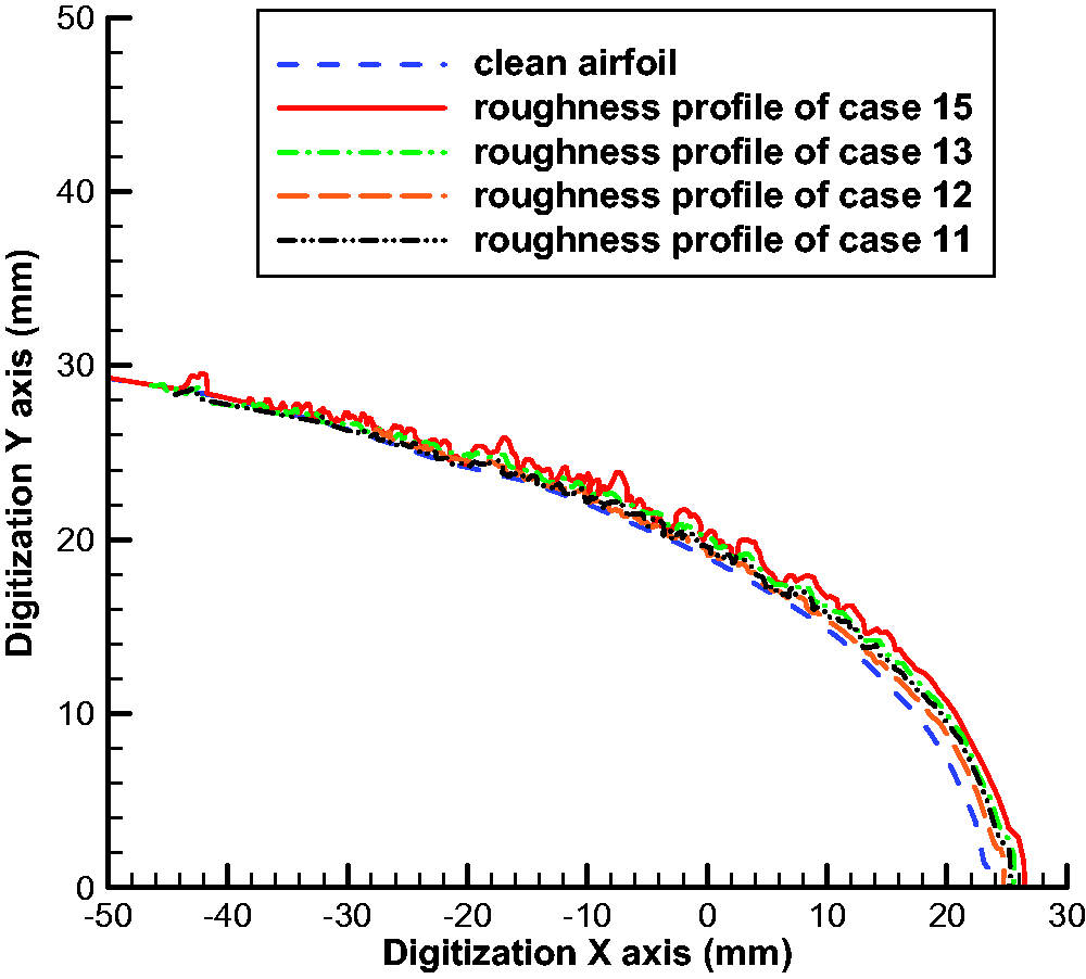
Different digitized roughness profile (See colour version of this figure online).
A common parameter used to describe the ice-induced surface roughness is the roughness element diameter,13,18,19 which is an average of hundreds of elements measured in the region right after the smooth zone based on the assumption that a single roughness element is a hemisphere. However, the diameter of the roughness element may not be a suitable metric in the present work. The present work only focuses on the ice-induced roughness at the early stage of the ice accretion, during which the roughness elements may have some different characteristics compared to well-developed elements. For example, the roughness elements were not observed to be nearly hemispherical in the present work (Figure 15); hence, the diameter of the elements is not particularly representative of the roughness height. Furthermore, the diameter of the roughness element does not appear to be directly connected to the broadband noise.
Consequently, rather than using the roughness element diameter, two different parameters were investigated in the present work to describe different ice-induced roughness heights at the early stage of the ice accretion, and as a correlation parameter for broadband noise level: (1) the arithmetic average of the roughness height Ra and (2) an averaged roughness height based on the accreted ice area (area under the roughness curve as shown in Figure 16(b)).
The arithmetic average of the roughness height Ra is commonly used in research areas such as tribology and lubrication. The formula for Ra is shown below when the roughness profile contains n ordered, equally spaced points along the trace

The mean line calculated in the present work is a moving average that averages a total number of 21 data points for the current point. The sample includes the current point, 10 data points before the current point, and 10 data points after. An example of the calculated mean line and the original digitized roughness profile is shown in Figure 18. The Ra values in Figure 18 are for the case 1 icing condition shown in Table 2.
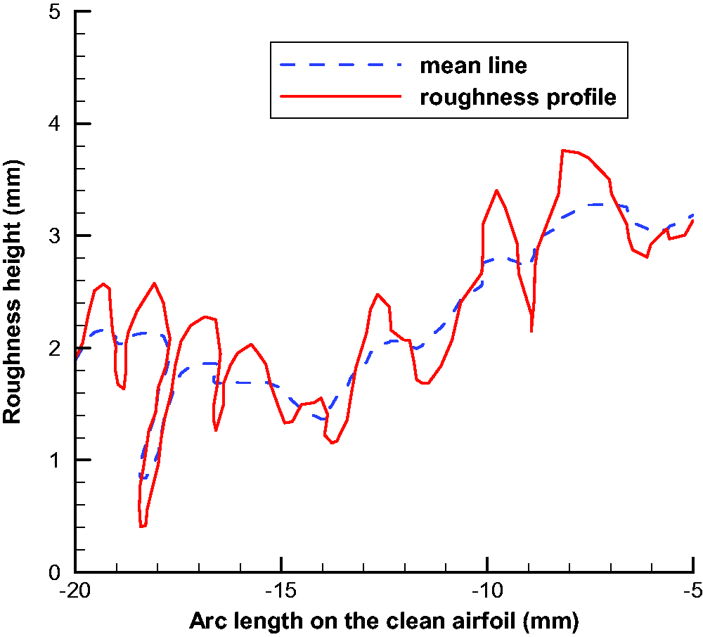
An example plot of the mean line and the roughness profile (case 1) (See colour version of this figure online).
The advantage of using arithmetic average of the roughness height Ra is that only roughness effects are considered because the mean height is removed; hence, the thickness of the ice layer in the smooth zone and the ice substrate under roughness in the rough zone will not contribute to Ra. This feature is expected to permit a better correlation relationship with the broadband noise, because the smooth zone near the stagnation point is considered to have little contribution to the broadband noise change, and this region is removed by using Ra.
The other parameter used is an averaged roughness height, which is the area of ice under the digitized measurement of the accreted ice surface (Figure 16(b)) divided by a constant perimeter 2πR (R is the airfoil leading edge radius and is 8.64 mm for the “paddle” blade). The constant circle perimeter used here is to follow the notation of Anderson et al., 19 in which twice the airfoil leading edge radius length is used to nondimensionalize the ice-induced roughness height. This roughness height can be treated as an “averaged ice roughness height” around a circle whose radius is that of the airfoil leading edge.
The roughness description parameter needed in the present work is used to correlate with the broadband noise, which is expected to be related to the boundary layer transition location as well as the boundary layer thickness at the trailing edge. However, there has not been any investigation to find where boundary layer transition takes place along the ice roughness, 13 and it is still not clear that whether the boundary layer transition is affected by the overall roughness or just the roughness in the rough zone. Even the ice layer thickness in the smooth zone could have a contribution to the change of the boundary layer characteristics, but the contribution (if any) is not currently known. To address these questions it is necessary to make detailed boundary layer measurements at different positions along the iced airfoil, but such measurements are beyond the scope of the present work. Due to the lack of knowledge of the detailed physics of the boundary layer and its dependence on the ice-induced roughness, the average roughness height used in the present work, which can be treated as an overall average height of the smooth ice layer height in the smooth zone, and the roughness height in roughness and ice feature zones, is considered to be an acceptable parameter to correlate with the broadband noise level.
The accreted ice area was treated as the area between the clean airfoil and the roughness profile. For each case, it was calculated by integrating the area between the roughness profile and the x-axis (clean airfoil arc) in the unwrapped digitized roughness profile, shown as the gray region in Figure 16(b). Values of the averaged roughness height based on such accreted ice area from different icing conditions are also shown in Table 3.
Ice-induced surface roughness height.

Subjective error in defining the clean airfoil and the roughness profile was estimated by comparing the results from two different digitizations of the same images. For those cases for which duplicate analyses were performed (cases 1–6), the maximum uncertainty indicated was less than 3% for the arithmetic average roughness height Ra and 5% for the accreted ice area. The uncertainty error percentage for each case is calculated by using the absolute difference of the concerned value between two digitizations divided by that the value of the first digitization. The concerned value is either Ra or the accreted ice area calculated from the digitization as previously presented.
One obvious concern for both description parameters used in the present work is that only the roughness at the blade tip is considered, rather than for the entire blade. This is thought to be reasonable because the airspeed was found to have little effect on the ice-induced roughness height, 18 which means the roughness on the rotor blades along a certain spanwise distance should not change much. This conclusion is confirmed in the present work by the observation that no significant ice roughness change is observed along the “paddle” blade span for any of the cases. Consequently, the present work assumes that the roughness change in the spanwise direction on the “paddle” blade test section (12 in. long, flow speed range 52.3–66.7 m/s) is negligible. It was observed that the ice roughness changed from the blade tip to the root; however, only the ice accretion on the “paddle” was considered in this work, and ice roughness on other sections of the rotor blade was removed before all broadband noise measurements. Furthermore, only the tip region is expected to contribute significantly to the broadband noise because the unsteady loading is expected to be highest at the tip due to the higher flow velocity over the blade surface.
2. Broadband noise level for correlation
The broadband noise level used in both correlations is an integrated MSP value (Pa2) in the frequency range from 10 to 24 kHz, shown as the gray region shown in Figure 19. The selection of the integrated frequency range is based on the earlier observations of the frequency range where the broadband noise of different roughnesses was distinct.
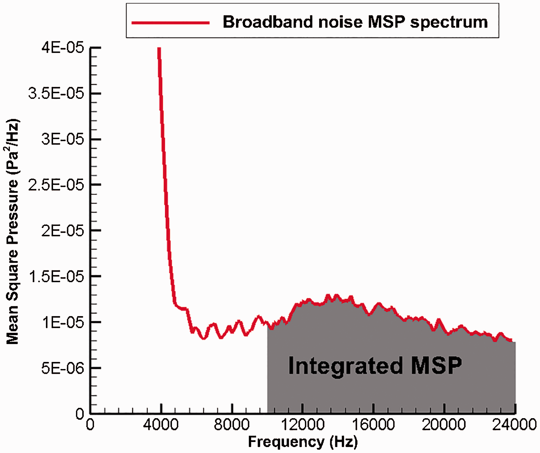
Integrated broadband noise level (case 1). MSP: mean square press (See colour version of this figure online).
3. Roughness and noise correlation
Ice-induced surface roughness and broadband noise level are then correlated. Figure 20 shows the correlation between the arithmetic average roughness height and the integrated broadband noise level. The point with zero arithmetic average roughness height (point on x-axis) represents the clean blade case. The 17% error from the broadband noise measurement indicated as the horizontal error bar is shown in Figure 20, while the 3% roughness digitization error is represented by the vertical error bar. The trend line is calculated based on the linear least squares method and is referred to as the correlation relationship for the prediction of the ice-induced surface roughness through measured broadband noise level. Its equation is given by y=10.36x−0.1775. The overall correlation relationship is a simple but strong positive correlation. The absolute mean deviation in percentage for this correlation data is 9.3%, which is calculated by the following formula

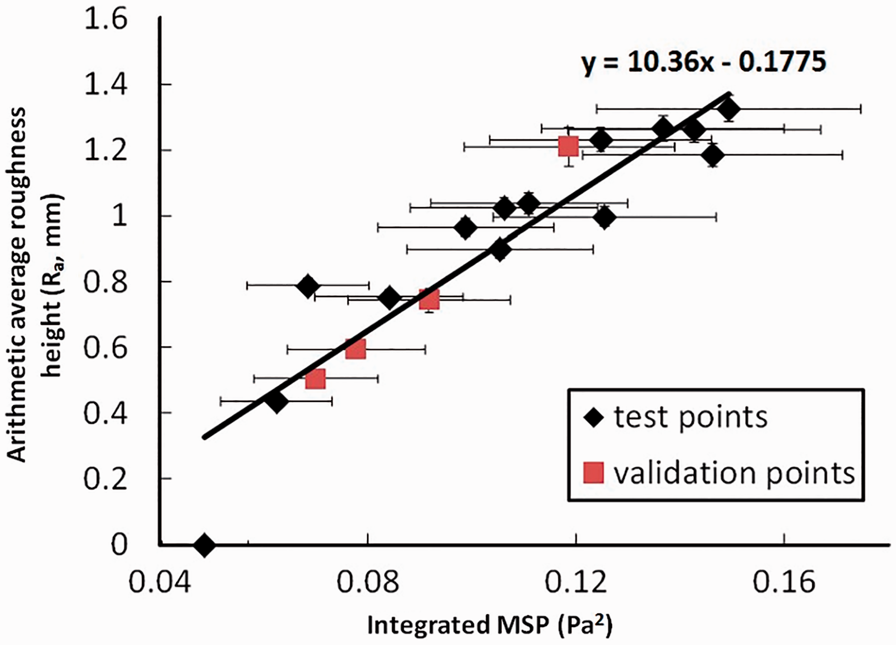
Correlation between the arithmetic average roughness height and the integrated broadband noise level. MSP: mean square press (See colour version of this figure online).
The four red square points shown in Figure 20 are the validation cases used to validate the developed correlation between the arithmetic average roughness height and the broadband noise level. They were not used in developing the correlation, yet a good validation trend is achieved, with a 7.9% absolute mean deviation.
Different averaged roughness heights, which are the accreted ice areas divided by a constant circle perimeter 2πR(53.16 mm), are also correlated to the integrated broadband noise level. The correlation result is shown in Figure 21. The roughness digitization error is 5% for this averaged roughness height (accreted ice area), which is represented by the vertical bar. The trend line equation is y=34.241x−1.1143. Similarly strong correlation results are obtained (as compared to Figure 20), with an absolute mean deviation of 11.2%. The Pearson correlation coefficient is 0.9592. The validation points fall almost exactly on the trend line, which shows a better validation with a 7.6% absolute mean deviation.
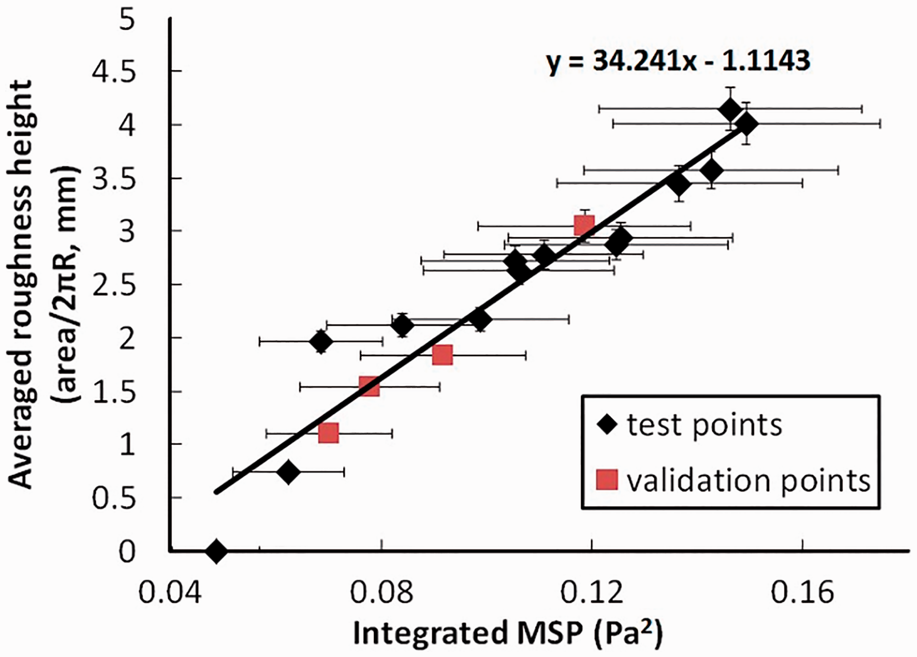
Correlation between the averaged roughness height based on accreted ice area and the integrated broadband noise level. MSP: mean square press (See colour version of this figure online).
Numerical investigation
CFD setup
Due to a lack of experimental measurements of the boundary layer thickness and turbulence intensity due to surface roughness, 2D numerical simulations were performed to investigate the effects of these on trailing edge noise due to surface roughness. For this work the commercial CFD software STAR-CCM+ 22 has been used. Steady, two-dimensional Reynolds-averaged Navier–Stokes (RANS) computations, with the SST k-omega turbulence model 23 were performed. Three different airfoil shapes at 0° angle of attack were investigated: (1) NACA 0012 clean airfoil with a chord length equal to 0.5334 m, which is the same as the “paddle” blade used in AERTS; (2) an NACA 0012 airfoil with small ice-induced surface roughness (case 15 in Figure 4 or Table 2); and (3) an NACA 0012 airfoil with larger ice-induced surface roughness (case 12 in Figure 4 or Table 2). The two roughened airfoil shapes are digitized from the iced airfoils as shown in Figure 4. Details of the ice shape digitization procedure can be found in Cheng et al. 1 A structured wall-layer resolved C-grid is used for all three airfoils. Grid examples of iced airfoils are shown in Figures 22 and 23.
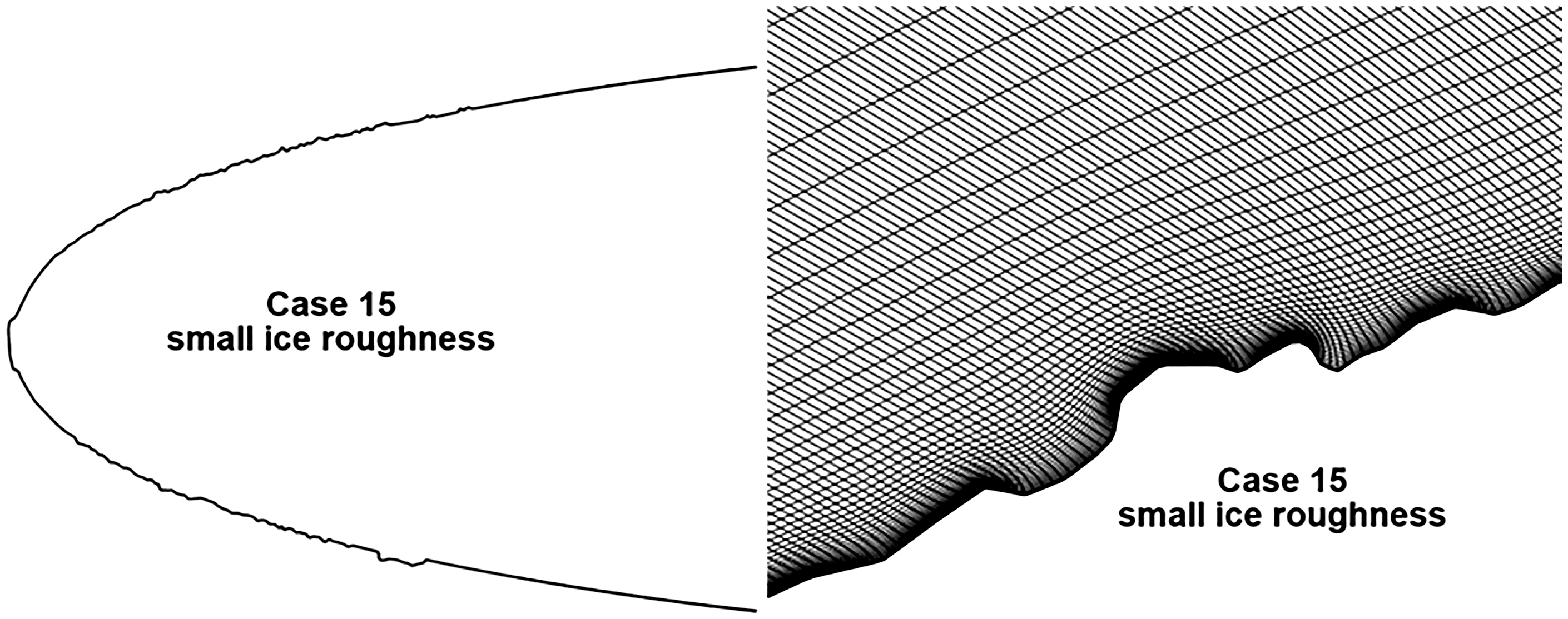
Structured grid of the iced airfoil with small roughness height (case 15).
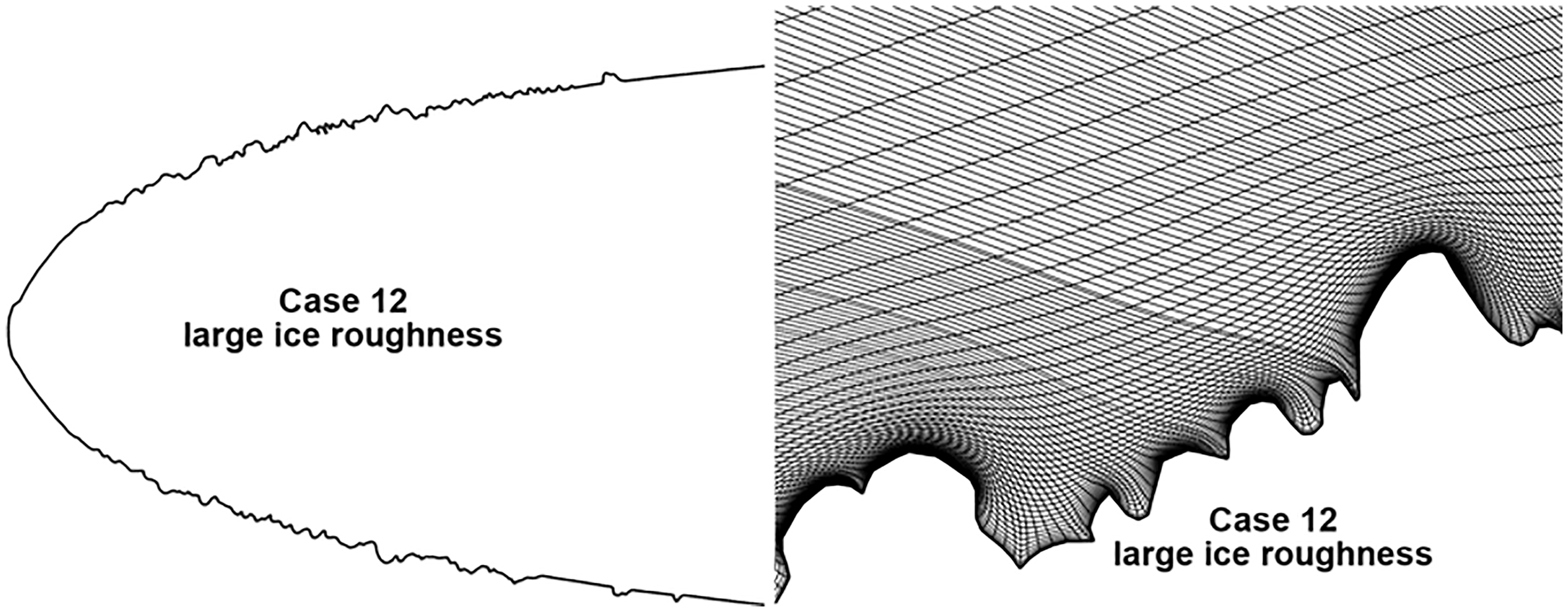
Structured grid of the iced airfoil with large roughness height (case 12).
CFD results
Trailing edge velocity profiles perpendicular to the chord line for the three different airfoil shapes are shown in Figure 24 for a freestream Mach number of 0.2. This Mach number is the same as the tip Mach number of the broadband noise test based on the ice-induced surface roughness performed in AERTS. Other Mach numbers are also simulated, but the results are not shown because the same boundary layer thickness trends are evident. Both iced airfoils have a larger boundary layer thickness than the clean airfoil, case 12, which has the largest roughness height and also has a larger boundary layer thickness than case 15. The boundary layer displacement thicknesses found from Figure 24 are 3.02 × 10⁻³, 3.44 × 10⁻³, and 4.85 × 10⁻³ m for clean airfoil, small roughness airfoil (case 15), and large roughness airfoil (case 12), respectively. This is the same trend seen in the increased SPL level as shown in Figure 9.
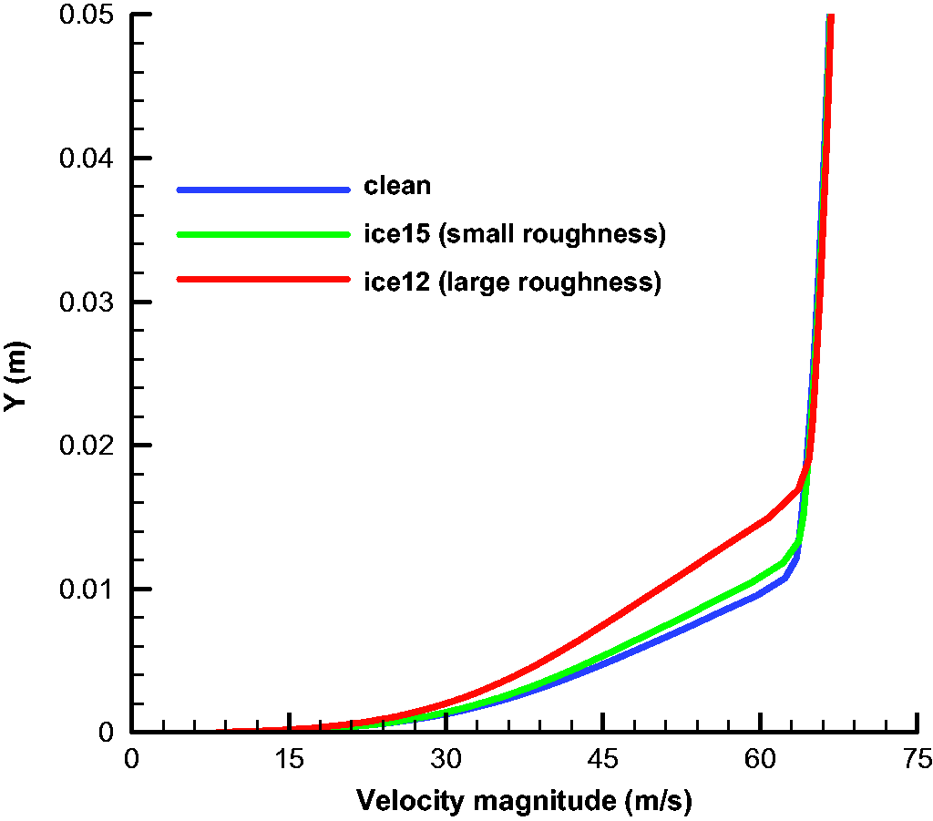
Velocity profile at trailing edge (Mach number = 0.2) (See colour version of this figure online).
Figure 25 shows the turbulence intensity of different airfoil shapes at the trailing edge for the Mach number 0.2 case. A normalized integrated turbulence intensity
24
is used to measure the level of turbulent kinetic energy at the trailing edge. This parameter is then used in Howe’s trailing edge noise scaling law to estimate the effect of the turbulence intensity on the trailing edge noise. The equation used to calculate the normalized integrated turbulence intensity is given by equation (2), where 
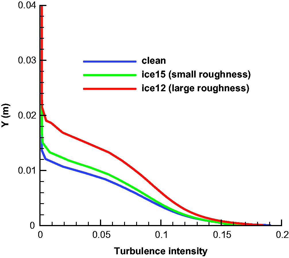
Turbulence intensity profile at trailing edge (Mach number = 0.2) (See colour version of this figure online).
Increased trailing edge noise estimation
Howe’s trailing edge noise scaling law (equation (5)) is used here to estimate the increased SPL due to the increased boundary layer thickness and the increased turbulence intensity. 
The estimated SPL increase results are shown in Table 4. The measured increases in SPL levels (as shown in Figure 9) at 18 kHz are also shown in Table 4 for comparison purposes. For case 12 with high ice-induced surface roughness height, the total estimated SPL increase (effects due to both displacement thickness δ1 and normalized integrated turbulence intensity
Increased trailing edge noise estimation.

Conclusions
Rotor broadband noise due to ice-induced surface roughness has been investigated experimentally. The noise source mechanism has been identified to be the TBL-TE noise. Trailing edge noise theory and CFD simulations are used to explain the experimental results that rotor broadband noise from higher surface roughness heights gives a higher SPL values. The following conclusions can be drawn:
Rotor broadband (trailing edge) noise increases due to surface roughness during ice accretion in high frequencies. Higher surface roughness height shows a higher SPL. The ice-induced surface roughness measurements are correlated to the measured broadband noise level from 10 to 24 kHz in the AERTS test. Strong correlations (the Pearson correlation coefficient of 0.9208 and 0.9592 for correlation using R
a
and the averaged roughness height separately) between the ice roughness and the broadband noise level are obtained, which can be used as a tool to determine the accreted ice roughness in the AERTS facility through acoustic measurement. It might be possible to use a similar approach to develop an ice accretion early detection tool for helicopters, as well as to quantify the ice-induced roughness at the early stage of rotor ice accretion. Two parameters are identified to explain the trailing edge noise increase due to surface roughness: (1) boundary layer (displacement) thickness, and (2) turbulence intensity. The effect of turbulence intensity on the trailing noise is greater than that from boundary layer thickness effects. Turbulence intensity should be considered in any trailing edge noise prediction model, especially for cases with surface roughness.
Footnotes
Authors’ note
The U.S. Government is authorized to reproduce and distribute reprints notwithstanding any copyright notation thereon. The views and conclusions contained in this document are those of the authors and should not be interpreted as representing the official policies, either expressed or implied, of the U.S. Government.
Acknowledgments
The acoustic test in the UMAC was supported by Dr Fred Schmitz, Dr Sudarshana Koushik, and Dr Richard Sickenberger.
Declaration of conflicting interests
The author(s) declared no potential conflicts of interest with respect to the research, authorship, and/or publication of this article.
Funding
The author(s) disclosed receipt of the following financial support for the research, authorship, and/or publication of this article: This research is partially funded by the Government under Agreement No. W911W6-11-2-0011.