
Abstract
This paper explores the effect of fan exit guide vane (FEGV) placement on the aft-radiated interaction broadband noise created by the turbofan stage. The Source Diagnostic Test (SDT) rig-scale fan stage configurations are analyzed. Simulations are carried out using two low-order methods, one based on methods developed by Stewart Glegg and the other one based on methods developed by Ventres, allowing a comparison between their predictions. Additional effects, including the influence of vane sweep, inflow turbulence inhomogeneity and turbulence length scale estimation methods are investigated. The simulations presented here support previous findings that show, unlike the tonal noise, the broadband noise is only slightly affected by the FEGV placement. Both low-order models show that FEGV placement has a tilting effect on the broadband spectrum but they predict different trends in overall sound power level. The spectral tilting is mostly influenced by changes in the turbulence length scale while the overall change in the spectral level is associated with the changes in annulus area. Therefore, as the FEGV placement changes, the final spectrum depends on the magnitude of each influence. Still, the overall broadband noise level only varies within the range of 1 dB for all FEGV cases and placements considered.
Keywords
Introduction
Advancements have been made on reducing turbofan engine noise and improving efficiency in the past decades.1,2 One of the major design changes that produces higher efficiency is increase in bypass ratio (i.e. increase in fan diameter). The modern and future ultra high bypass ratio (UHBR) engines have shifted the dominant noise source from jet noise to fan noise. Along with larger fan diameters, modern engines tend to have shorter nacelles to reduce the weight and drag penalties. One way this can be achieved is by reducing the fan stage gap, which involves considerations of shape and placement of the fan exit guide vanes (FEGVs) during engine fan stage design.
An early study using the full-size QF-5 fan showed that FEGV placement has considerable effect on the bypass tonal noise. 3 This finding was also supported by the Allison fan experiment.4,5 The tonal noise decreases with FEGV distance from the fan because the wake deficit decays as the wake evolves. Broadband noise on the other hand has been shown to be less dependent on FEGV distance from the fan.6,7 Indeed, the overall acoustic broadband power was shown to change little as the distance between the FEGV and the fan decreased in the more recent ACAT1 test rig.6,8 Little change in the overall broadband noise level as the interstage gap is decreased is a rather favorable phenomenon, because shorter gaps reduce engine weight; and while a shorter gap promotes higher tonal noise, tones can be damped via duct geometry and acoustic liners.
This paper focuses on how gap length and geometry affect the broadband noise. It also provides an opportunity to compare two methods that have been described in the literature for computing broadband fan noise. The fan used in the study is the NASA Source Diagnostic Test (SDT) rig. 9 In the SDT experiments, three FEGV configurations were tested, 54-vane straight (baseline, BL), 26-vane straight (low-count, LC), and 26-vane swept (low-noise, LN). Performance and noise were measured. While the effect of FEGV axial position on broadband noise was not the focus of the SDT experiments, the full fan stage geometry is available and allows for modifications of FEGV placement for simulation purposes.
The study presented in this paper is an extension to an earlier work. 10 In this paper, the predictions of the SDT fan stage exhaust broadband interaction noise are made using two low-order acoustic models. This provides an opportunity to compare the performance of these two methods. The first model is the rotor-stator interaction noise (RSI) model11,12 and the second is Hanson’s model 13 as it is coded in OptiSound. 14 Hanson’s model is built upon the broadband cascade response method developed by Stewart Glegg. 15 Indeed Glegg has contributed heavily to the field of fan noise by developing fan-alone broadband noise models,16–18 as well as the foundations for Hanson’s model for fan-stage broadband noise.
Both fan-stage broadband noise methods used in this work require fan wake flow information to be known and then compute the FEGV response to the fan wake inflow. Here, rotor-alone Reynolds-Averaged Navier-Stokes (RANS) simulations provide the fan wake flow. Hanson’s method allows for analysis that includes passagewise variation of the fan wake turbulent kinetic energy and turbulence length scale. The effect of including these inhomogeneities is explored in the paper.
In the next section, the SDT rig is briefly described, then the two low-order broadband acoustic prediction methods are introduced. The fan wake data used as input for the low-order calculations are described in the RANS data extraction section. The Results section explores several related and important parameter choices and FEGV characteristics. Finally the vane placement results are shown.
Methods
Fan-stage configuration
SDT FEGV configurations.

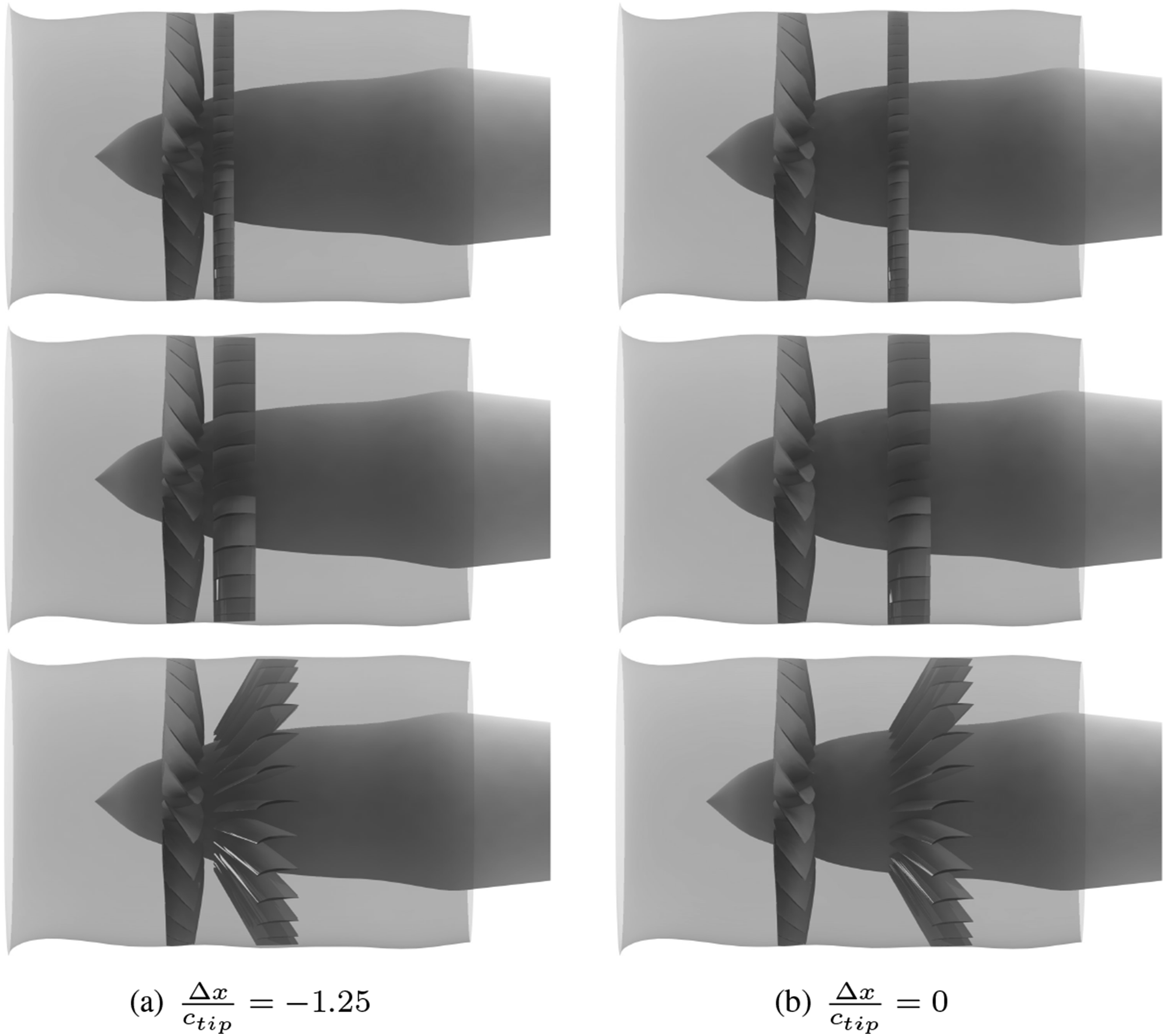
SDT fan stage configuration. (a) Closest modeled location of the FEGV. (b) SDT FEGV location in the experiment. From top to bottom: baseline, low-count, low-noise.
Operating points and baseline vane stage pressure ratios from RANS.

Analytical methods
The broadband noise analysis presented in this paper focuses solely on the interaction noise produced by the interaction of the fan-wake turbulence with the FEGV. The predictions from two low-order cascade models are compared: (1) the BU-RSI model that is based on Ventres’ cascade response function and uses duct mode propagation via the Green’s method, and (2) the OptiSound/Hanson’s model that is based on Glegg’s cascade response function and uses free-field propagation.
BU-RSI
The BU-RSI model is based on the formulation by Ventres et al. 20 and later improved by Meyer, 21 Envia & Nallasamy, 11 and Grace. 12 Ventres provided an integral equation for the unsteady blade loading of a 2D cascade to an incident 2D gust with displacement normal to the vane and convected by the mean flow.
A simplified view of an FEGV unrolled spanwise slice is shown in Figure 2. Ventres’ method assumes that the mean flow is aligned to the strip (i.e. that there is no radial flow), so that k1 ≈ ωc/2U(r). The Ventres’ method can be extended to account for 3D gusts
12
using Graham’s similarity rules. Graham’s method uses a transformation between the actual 3D gust problem and a related 2D gust problem. It is possible to extend this method to account for swept vanes. There is however, some ambiguity when applying the transformation. The ambiguity is explored in this paper. More information is given in the Appendix. Cascade definition.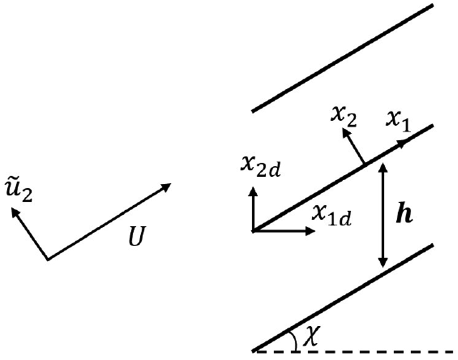
For fan-stage broadband noise, where fan wake turbulence is driving the FEGV response, the turbulence is represented in the wave-number frequency domain such that each component can be treated as a single gust. The FEGV response to each gust is built using the strip theory where each radial slice is treated as a flat-plate cascade. The stagger of the flat-plate cascade is set to match the mid stagger value at each radial location. Previous work7,12 showed that although the choice of stagger definition, i.e., leading edge, trailing edge, or a weighted combination of both, influences the prediction, the stagger definition does not change the trend from one flow condition to another.
The gust or upwash amplitude at each radial strip is modeled by the Liepmann turbulent velocity spectrum. The parameters required to define this spectrum at each radial location are determined from RANS simulations of the fan alone and will be discussed below.
The Green’s function is singular at many frequencies. A preprocessor is used to select nonsingular frequencies. It uses a set criterion for the offset from a singular frequency. The aim is to acquire results in the troughs between singular frequencies. However, this process is not perfect and we have not corrected the spectrum when a trough is not identified correctly. As such, the BU-RSI results can be a bit ”spiky”, especially in the 1 kHz to 2 kHz range.
Hanson
The Hanson model available in OptiSound TM is an extension of Glegg’s 15 asymptotic formulation. In contrast to Ventres’ method that solves vane surface pressure, Glegg’s method solves for the velocity potential on the flat-plate cascade using the Wiener–Hopf method. The method handles 3-D gusts with swept and leaned vanes. Another model also based on Glegg’s formulation, Posson’s model 22 is also implemented in the OptiSound software, but is not considered in this study.
In Glegg’s coordinate system, sweep and lean are handled by rotating the frame of reference. For a swept vane for example, the entire strip rotates along the x2 axis, accompanied by a transformation in coordinates with varying blade distances along the chord as illustrated in Figure 3. This also implies that the effective chord length becomes c cos (ψ
s
), and the effective chordwise velocity becomes U cos (ψ
s
) and additional spanwise velocity U sin (ψ
s
) and spanwise wavenumber sin (ψ
s
)ω/U are created where ψ
s
is the sweep angle. Finally, unlike the BU-RSI model in which duct modes are being computed, Hanson’s model considers free-field propagation. Sweep transformation in Hanson’s model.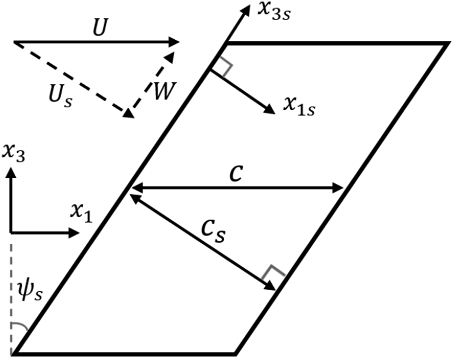
Hanson extended Glegg’s model by including passagewise turbulence inhomogeneity where the turbulence intensity can be modeled using the Gaussian function. The OptiSound implementation allows wake and background values to be specified for both turbulence intensity and length scale.
Because of the ability to include passagewise variation of the turbulent parameters, there are options available to the user. In this paper we will compare three inflow turbulence modeling methods: (1) locally homogeneous: both turbulence intensity and length scale are fully averaged circumferentially at each radial location; (2) inhomogeneous: Gaussian modeled turbulence intensity with circumferentially averaged length scale; (3) inhomogeneous: Gaussian modeled turbulence intensity with two averaged length scales discriminated by the 20% turbulent kinetic energy (TKE) Gaussian peak threshold.
RANS data extraction
The wake flow parameters downstream of the fan are simulated using the UTCFD code, 23 by solving the steady RANS equations (k − ω turbulence model) in a rotating frame of reference. The flow parameters are extracted from the RANS solution at the location where the leading edge of the FEGV would be. It is noted though that this method ignores any potential field effects that the FEGV's presence has on the fan wake. This method has been employed in previous work. The grid and the computational method are described in Li et al. 24
Figure 4 depicts the downstream duct geometry as well as the circumferentially averaged flow fields for the SDT configuration at the Approach condition. The horizontal axis represents the nondimensional relative FEGV location. The vertical axis represents the nondimensional radius. The duct area slightly pinches as the distance from the fan increases. This pinching effect becomes much greater beyond the design FEGV location, which leads to a notable axial flow acceleration. This is captured in Figure 4(a). Circumferentially averaged wake flow in the interstage gap based on RANS solutions. Approach condition shown.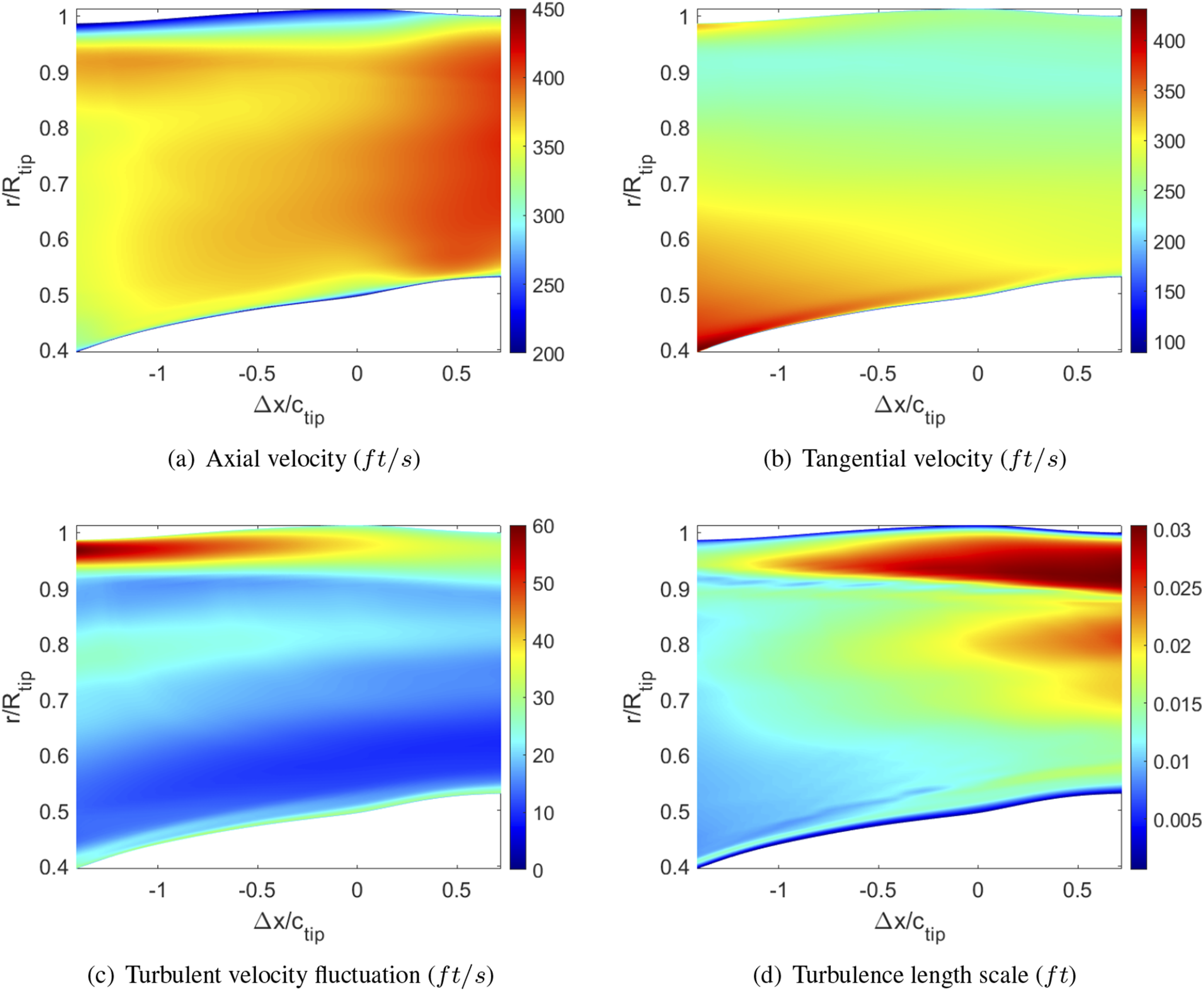
Isotropic turbulence is assumed, and the turbulent velocity fluctuation u′ is equal to
The k − ω-based turbulence length scale, Λ
k
, is estimated by Pope’s
25
formula,
The turbulent kinetic energy and turbulence length scale on a passage extracted at the constant axial location of Δx/c
tip
= 0 are shown in Figure 5. In Hanson’s model, when turbulence inhomogeneity across the passage is included, the turbulence intensity is modeled via the Gaussian function. This is done by fitting the computed passage TKE to the expected form: Turbulent kinetic energy and length scale passage fields at the Approach condition and design location. (a)TKE (b)Λ. Inhomogeneous wake modeling. Design location mid-span shown.
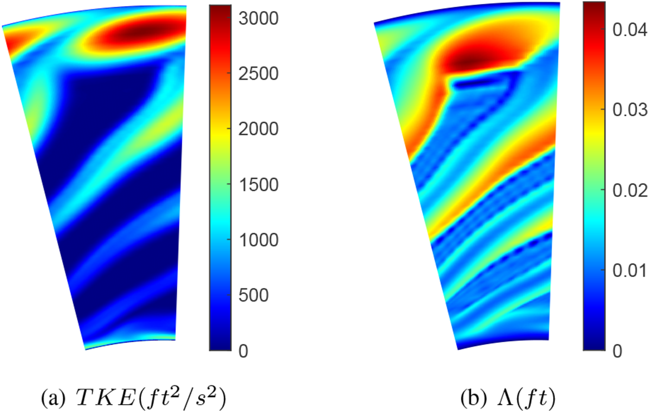
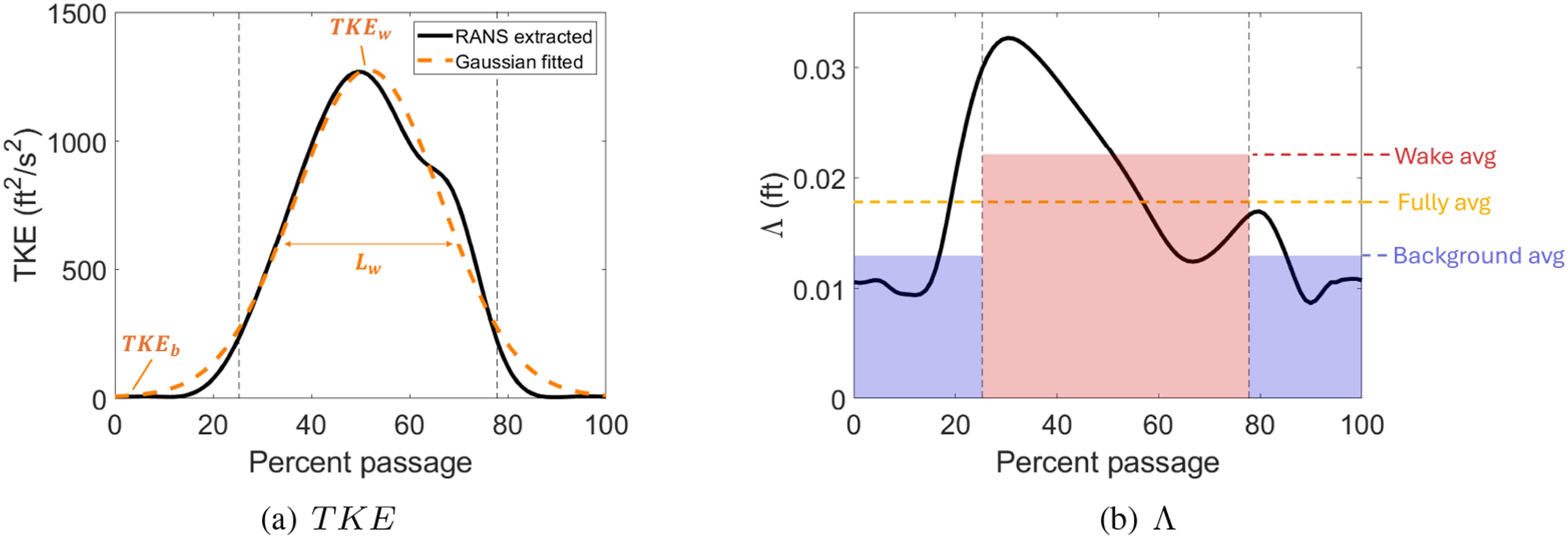
Likewise, the passage turbulence length scale can be either represented by a homogeneous value or separated into wake and background components. Figure 5(b) shows the Λ k passage slice. The fully averaged value at midspan is shown as the orange line in Figure 6(b). For the discriminate-average method, two averages are computed as in Leonard et al. 26 The vertical dashed lines in Figure 6 denote the threshold determined by the 20% Gaussian amplitude. Figure 6(b) shows passage Λ k where the background and wake averaged Λ k are represented by the shaded values. However, the Gaussian function is unsuitable at certain locations where the wake is not well-defined, such as near the shroud and hub as shown in Figure 5(a). The discriminate approach therefore is only being applied at radial locations where the passage TKE can be fit by a Gaussian function. The cut-off criteria are determined by the Gaussian fitting error as well as the ratio between the TKE b and TKE w to avoid locations where the wake is contaminated by the wall boundary layer and tip vortices.
Results
Effect of modeling passage-wise inhomogeneous turbulence
As discussed in the previous section, Hanson’s method models passage-wise inhomogeneous wake flow, though one could also use it to model locally homogeneous wake flow by defining just background turbulence parameters. Figure 7 shows the predicted broadband noise for the SDT baseline vane configuration at the Approach condition fan speed when the fan wake is modeled in different ways. The homogeneous method is plotted as the solid line (uniform), and the two inhomogeneous methods described above are plotted as dashed and dotted lines. The largest difference is attributed to modeling the u′ as inhomogeneous on the passage (difference between solid and dotted lines). It leads to a slight tilt in the sound power spectra. Typically, the tilt is attributed to the turbulence length scale. However, here, the different wake and background turbulence intensities influence the upwash velocity spectra in a way that also tilts the spectrum. Sound power spectrum using baseline vane at the Approach condition, Hanson’s model at Δx/c
tip
= 0 (design location).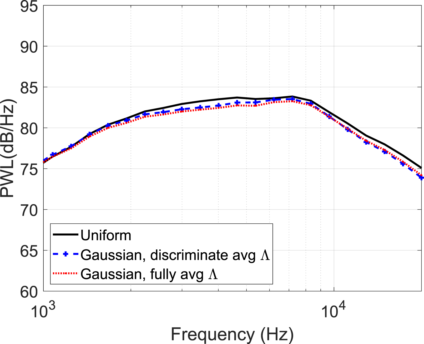
The influence of modeling passage-wise inhomogeneity of the turbulence intensity depends on the wake width. A thinner wake width leads to a larger impact on the result. This effect can be better seen in two ways. First, the wake at the Sideline condition is much thinner than at the Approach condition. The results for the Sideline condition in Figure 8(b) can be compared to the results for the Approach condition in Figure 7. For the Sideline condition, it is easily seen that there is a large difference between the time-averaged turbulence intensity case and the Gaussian distribution case (solid vs dotted lines). Second, the fan wake is thinner nearer the fan. Figure 8(a) shows the results when the SDT FEGV is moved upstream towards the fan (solid and dotted lines). Comparing Figure 8(a) & (b) shows that there is a larger difference in PWL between the different methods when the FEGVs are positioned closer to the fan. Sound power spectrum using baseline vane at the Sideline condition, using Hanson’s model.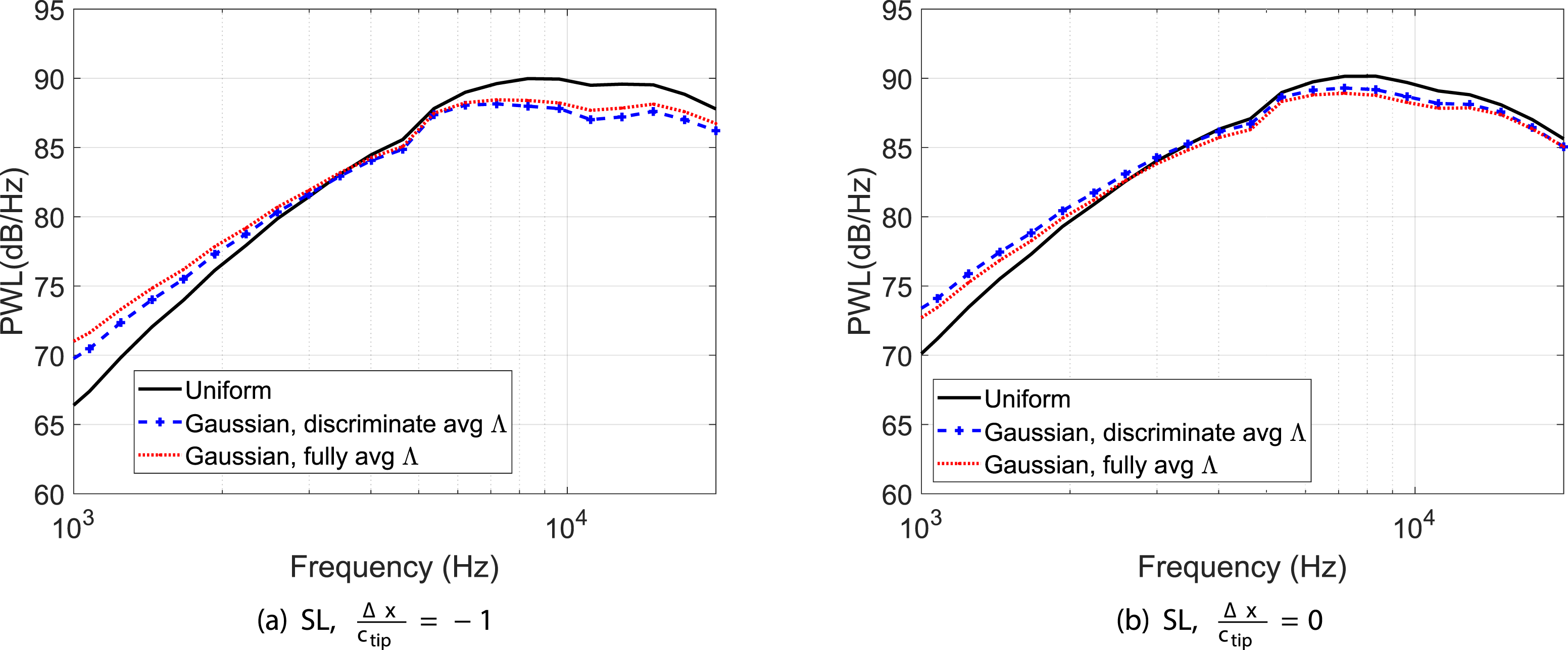
Effect of turbulence length scale estimation methods
In the previous section, the influence of allowing the turbulence length scale to vary between the background and wake center values was shown to have insignificant impact as seen in the dashed and dotted lines in Figures 7 and 8. In this section, the effect of using a completely different method to estimate the length scale is investigated. The first method was described above and uses time-averaged turbulence kinetic energy and dissipation rate from the RANS simulation, Comparison of turbulence length scale estimation methods. Approach condition at Δx/c
tip
= 0 showed.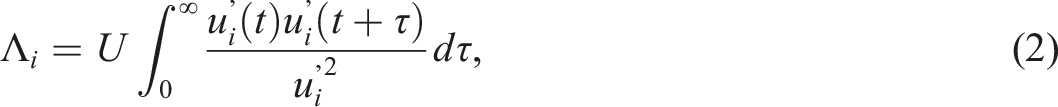
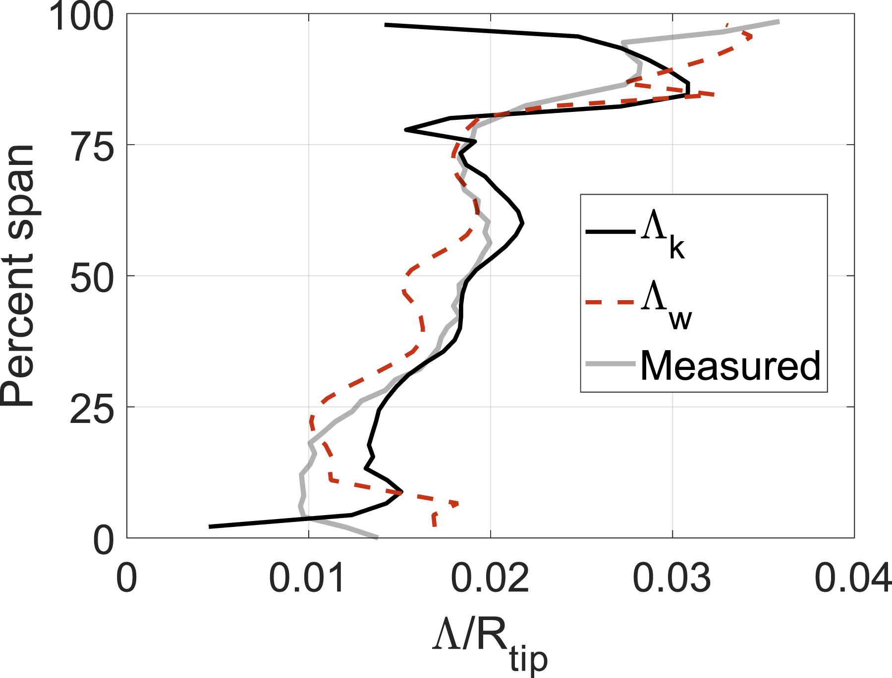
The predictions when using different length scale definitions are shown in Figure 10 for the (a) Approach and the (b) Sideline conditions. Both models show that the wake width method for defining the length scale, Λ
w
, leads to higher sound power predictions at low frequencies and slightly lower sound power predictions at high frequencies. The trend agrees with what was presented by Leonard et al.
26
and Lewis et al.
28
Figure 9 includes the experimentally measured spectra. Based on the experimental data, both methods seem to predict reasonable length scales. A drawback to the k − ω-based method is that Λ
k
is highly dependent on the RANS turbulence model. A good demonstration of this point can be found in the ACAT1 benchmark summary,
29
which shows that the Menter SST k − ω model typically predicts lower length scale compared to the Wilcox k − ω model. The difference between acoustic predictions using Λ
w
and Λ
k
, shown in Figure 10, is mainly driven by the length scale near the tip, where the wake shape is not well-defined due to tip vortices, leading to a larger Λ
w
estimation. It is also questionable whether or not Jurdic’s empirical model is applicable in the tip region. Therefore, in this work where we have a reliable Wilcox k − ω model, we chose to use the k − ω-based method. Comparisons of PWL spectra using different length scale estimation methods. 59 Hz bandwidth, Approach condition at Δx/c
tip
= 0.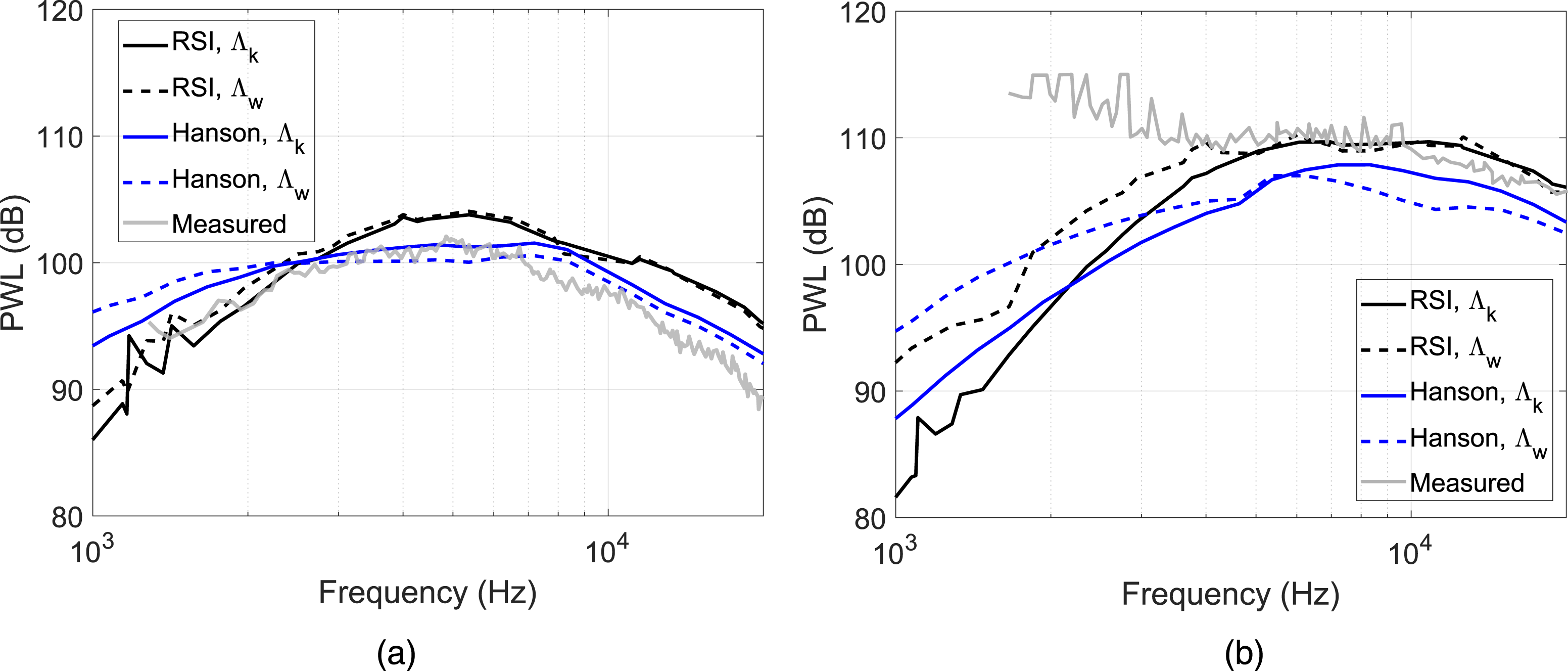
Figure 10 shows the predictions from both the Hanson and BU-RSI methods when using different length scale determination methods, together with the experiment-measured stage exhaust sound power. Interestingly, Hanson’s method appears to predict the Approach condition well, while the BU-RSI method predicts the Sideline condition well. As expected, the RSI model predicts lower power compared to Hanson’s model at low frequency because very few annular modes are cut-on. However, the difference between the two models at high frequencies is still under investigation.
Effect of vane sweep
The influence of sweep on broadband noise can be broken down into two components: (1) The effect of mean flow at the leading edge and (2) the vane response due to a skewed gust. The difference in mean flow is being discussed first. The inputs used for the acoustic models are extracted from the CFD solutions along the vane leading edge at the design location (Δx/c
tip
= 0). Figure 11 shows that the longer distance between the swept vane LE and the fan results in a slight decay in the circumferentially averaged turbulence intensity (f) and expanded turbulence length scale (i). The swept vane extends further downstream where the axial mean flow (a) accelerates due to the pinched duct geometry. Normalized inputs extracted from RANS CFD solutions along the vane leading edge for LN and LC vanes at the SDT experimental location at Approach condition. (a)-(b) Mach number, (c) Wake width, (d)-(f) Turbulence intensity, (g)-(i) Turbulence length scale.
The results for the power spectrum computed using the BU-RSI and Hanson’s method for three characteristic operating conditions and the LC (blue) and LN (cyan) vanes are shown in Figure 12. If one just changes the inflow to reflect the change in the wake flow along the leading of the FEGV, but treats the vane as a straight vane in the model, one would obtain broadband noise predictions shown as the black dashed lines in Figure 12. An argument for such a calculation is the fact that the turbulence is supposed to be decorrelated from strip to strip and so each cascade could be seen to act similarly whether it was part of a straight or swept vane. Comparing the black line to the red line, which gives the results for a straight FEGV with the wake flow along its actual leading edge, one sees the inflow difference leads to higher broadband noise with the swept vane inputs. This does not reflect the experimental results. SDT LC and LN downstream acoustic power using the BU-RSI model and Hanson’s model. 59 Hz bandwidth.
Fully modeling the swept FEGV however, leads to the more physical prediction of a slightly lower broadband noise level represented as the black solid line. The difference seen with the Hanson model, which adopts Glegg’s coordinate system as shown in Figure 3, comes from the reduction in the chordwise mean velocity component and the effective chord length together with the addition of the spanwise flow component and wavenumber. The BU-RSI model utilizes the same rotated coordinate system (see Appendix) such that sweep transforms the effective chordwise wave number and the range of spanwise wavenumbers that can radiate but does not directly utilize the spanwise flow component to redefine the effective frequency.
For the cutback and sideline fan speeds, the predictions and experimental data diverge below 4 kHz. Others have shown that interaction noise generated by the rig support pylon is significant 30 at lower frequency especially for higher fan speeds. In addition, the ACAT1 benchmark study 8 also reported that analytical interaction noise models typically underpredict sound power level at low frequencies because the experimental measurement often includes low frequency noise sources that are not modeled. It is believed that the notable discrepancy between measured and predicted spectra under 3 kHz in Figure 12(c)-(f) as well as Figure 10(b) is at least somewhat attributed to the rig noise contamination in the experiment.
Effect of vane placement
Previously, researchers analyzed the ACAT1 fan stage as it pertains to FEGV placement. It was found that moving the FEGV closer to the fan did not result in a large noise penalty. Behn and Tapken 6 pointed out that moving the FEGV closer to the fan produces slightly higher noise levels at high frequency and lower levels at low frequency. The difference across the spectrum was less than 2 dB. This effect was corroborated by Blázquez and Corral. 31 The low-order BU-RSI method was used in a preliminary investigation of this effect in Li et al. 10 In this section, we aim to present a more comprehensive study of this topic.
The hub and tip radii in the acoustic models are defined by the duct geometry where the FEGV leading edge is placed. This implies that the annulus geometry defined in the acoustic model changes slightly as the FEGV placement moves. In the swept FEGV cases, the outer annular radius is defined by the duct radius at a slightly further axial location compared to the straight FEGV placed at the same hub location. The effect of these slight FEGV spanwise length differences on the final acoustic outcomes have been shown to be quite small. 7
Specific normalized locations downstream of the fan at which the FEGV might be placed are selected. They represent three shorter interstage cases compared to the original SDT. At each location, the wake flow parameters along the leading edge of the BL or LC and along the swept leading edge of the LN FEGVs are shown as line plots in Figure 13. Normalized wake flow inputs at Approach condition along the FEGV leading edge. (a)-(b) Mach number,(c) Wake width, (d)-(f) Turbulence intensity, (g)-(i) Turbulence length scale. Solid with pluses: 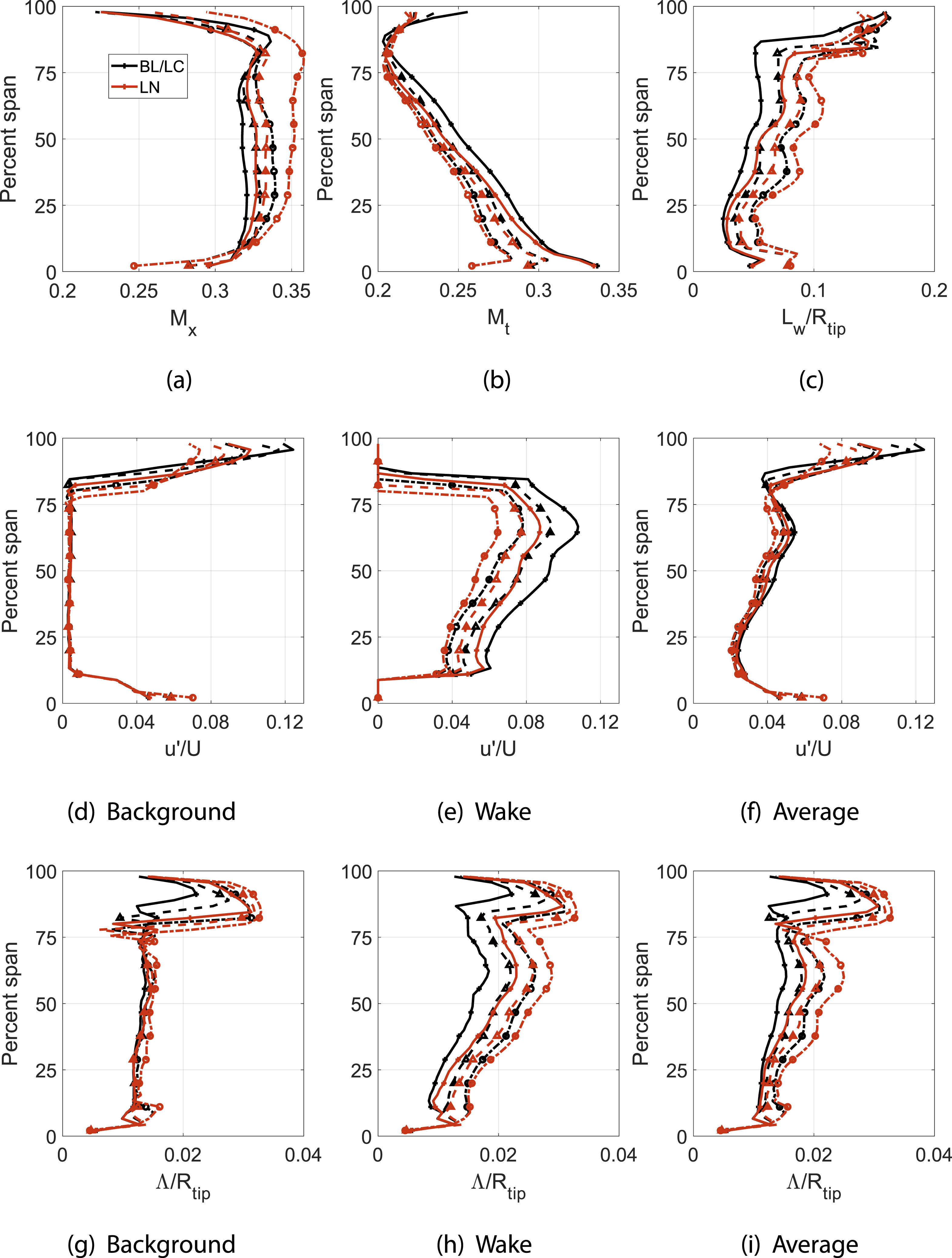
Again, the inputs (a), (b), (f), (i) are used when the inflow is modeled as locally homogeneous, and (a), (b), (c), (d), (e), (g), (h) are used when the Gaussian wake model is used. The line plots highlight the increase in axial velocity and turbulence length scale and a slight decay in turbulence intensity, with increased distance from the fan. For the Gaussian wake model, the decay in turbulence intensity occurs mostly in the wake amplitude while the background remains largely the same. Notably, the flow acceleration is much greater along the swept LN vane leading edge compared to the straight BL/LC vane leading edge, because part of the LN vane extends further into the region where the duct area shrinks at a steeper rate.
In Figure 14, the effect of vane placement on the downstream noise spectrum is shown for the BL vane as predicted by the different methods. The main influence on the acoustic prediction, as the location changes, comes from the turbulence length scale, which is responsible for the tilt of the spectrum. A larger length scale increases the low-frequency noise and decreases the high-frequency noise. Both models using Λ
k
show consistent trends. The wake width L
w
expands at a similar rate to the circumferentially averaged Λ
k
. As discussed in Section Effect of turbulence length scale estimation methods, determining L
w
near the tip is quite challenging, and the predictions using Λ
w
lead to different trends in the spectral shapes. It is reiterated that Λ
k
provides a more consistent length scale estimation. SDT baseline vane configuration sound power spectra at Approach condition. Solid: 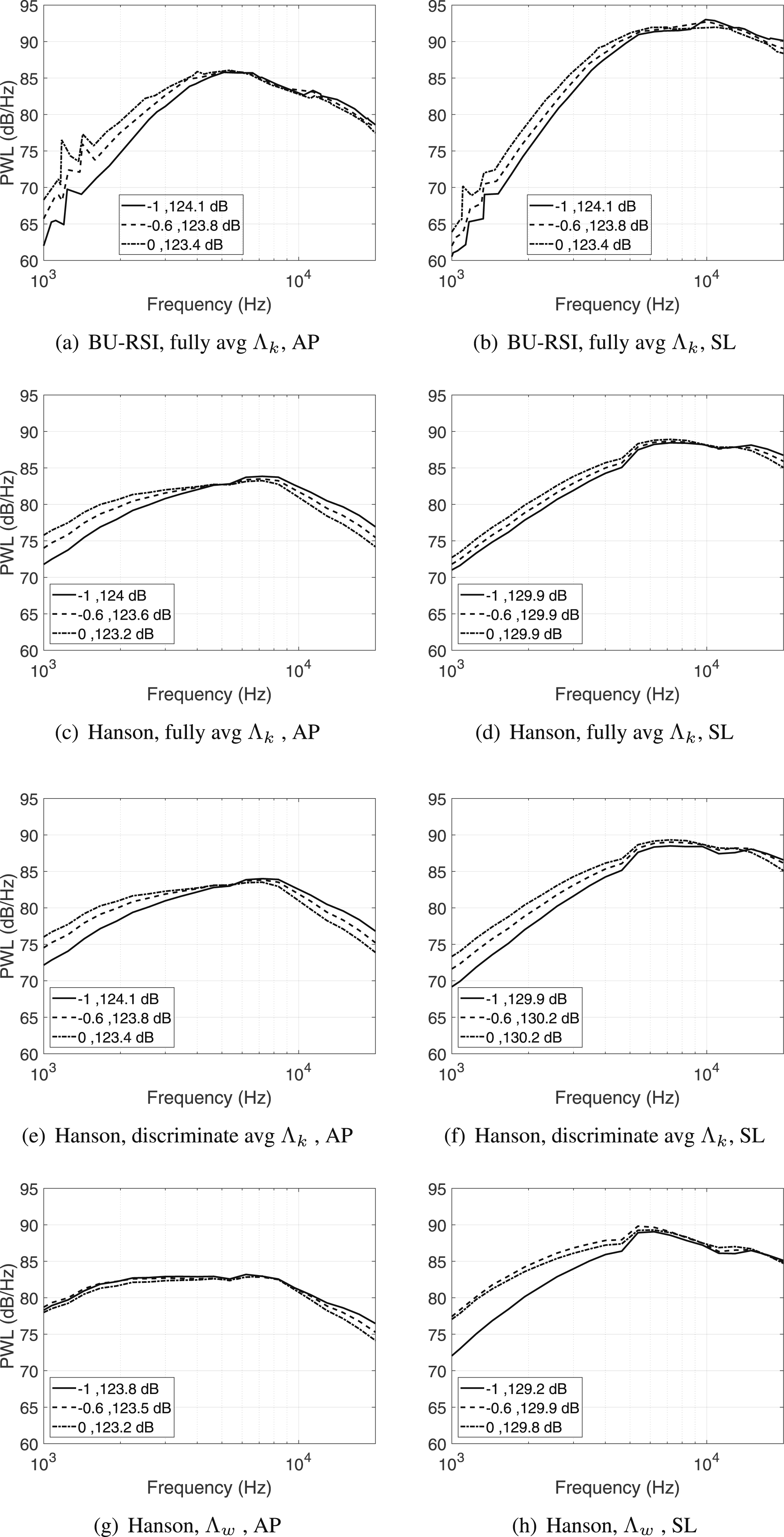
The results predicted using Λ k are in qualitatively good agreement with the experimentally measured spectra for ACAT1 using short and long gap configurations as reported in Behn and Tapken, 6 where placing the vane further from the fan increases the low frequency noise, and decreases the high frequency noise. Using Hanson’s model, with the wake turbulence treated as homogeneous or inhomogeneous leads to very similar trends. Quantitatively, the discriminate-averaged length scale approach leads to slightly shifted trends at higher frequency. This trend is more noticeable for the Sideline condition.
The noise prediction for the Approach operating point is shown in a slightly different way in Figure 15. Here, the spectra obtained when the FEGV is placed at different axial locations are compared to the spectrum at the design FEGV location. Hence the colormap depicts a Δ of the sound power spectrum compared to the spectrum when the FEGV is at Δx/c
tip
= 0. The BU-RSI model and Hanson’s model using the Gaussian wake and discriminate averaged Λ
k
are being compared. Hanson’s model shows a smoother result compared to the BU-RSI model due to the absence of duct singularity issues. Both models show similar trends qualitatively. When the interstage gap is shorter than the design gap, i.e. Δx/c
tip
< 0, the low frequency noise decreases and the high frequency noise increases. For the longer gap, i.e. Δx/c
tip
> 0, both models show the noise increases, especially at low frequency. Quantitatively, the BU-RSI model shows slightly less increase for a shorter gap at high frequency. This is tied to the difference in how the inflow mean velocity affects the prediction from each model, as discussed in a previous study.
10
SDT ΔPWL (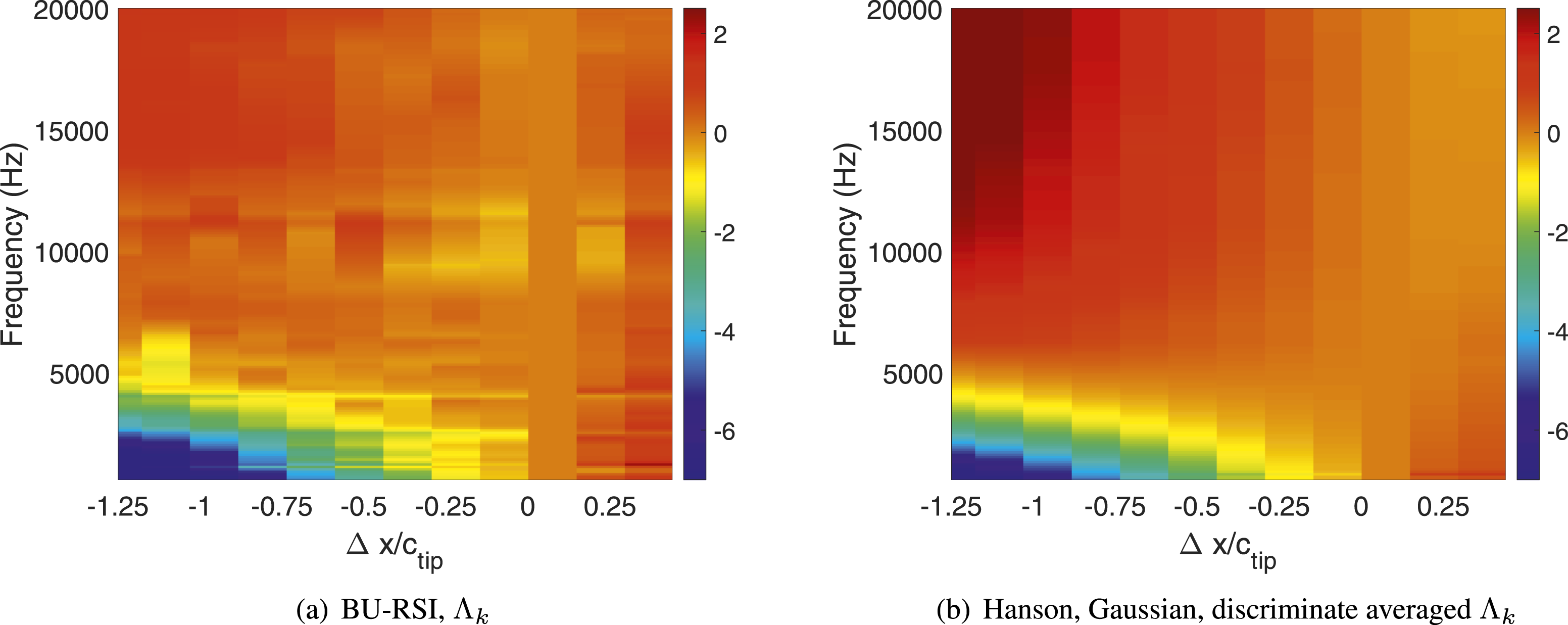
The overall sound power level (OAPWL) is calculated by integrating the spectrum up to 20 kHz. Figure 16 shows the predictions for the SDT BL vane from the BU-RSI model and Hanson’s model, using a Gaussian wake with discriminate averaged Λ
k
. Both models predict that the OAPWL change is basically less than 1 dB as the vane placement changes. Hanson’s model predicts overall lower OAPWL compared to the BU-RSI model. The difference in OAPWL, ΔOAPWL, referenced by the design location is depicted in Figure 17. At the Approach condition, the BU-RSI predicted values show that the OAPWL barely changes from Δx/c
tip
= −0.4 to 0, while Hanson’s model shows a slight decrease in OAPWL with distance of the FEGV from the fan. In this region the duct area change is small. Beyond the design location, Δx/c
tip
> 0, the duct area reduces rapidly and both models show an increase in OAPWL with distance due to flow acceleration. Modeling the inhomogeneous wake turbulence intensity has a rather small effect on ΔOAPWL at the Approach condition. At the Sideline condition, a Gaussian modeled wake with discriminate averaged length scale used in Hanson’s model leads to a slightly larger difference in ΔOAPWL compared to the other inflow definition options. OAPWL (left) and ΔOAPWL (right) as functions of normalized FEGV placement using baseline vane. Solid: RSI model, Λ
k
. Dashed: Hanson’s model, Gaussian wake, discriminate averaged Λ
k
. ΔOAPWL using baseline vane at Approach speed. Black: BU-RSI model, blue: Hanson model with homogeneous turbulence, blue-dashed: Hanson model using Gaussian turbulence with discriminate averaged Λ, blue-dotted: Hanson model using Gaussian turbulence with fully averaged Λ.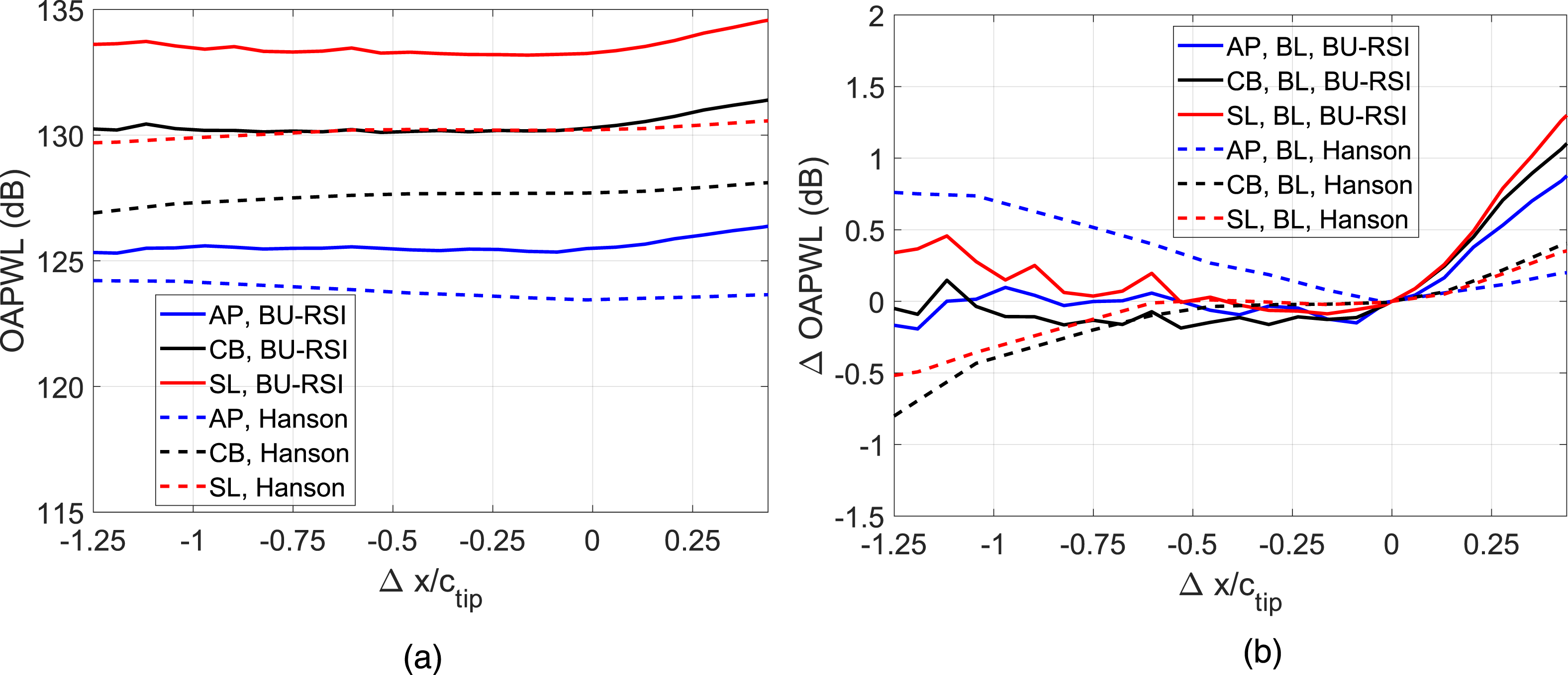
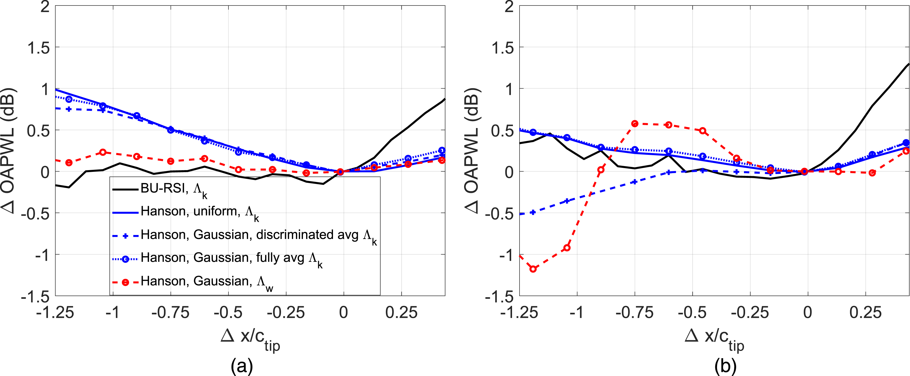
Figure 18 shows the predicted spectrum for the LC and LN FEGVs placed at the same axial locations. Results for the Approach operating condition are shown, and the methods being compared are the BU-RSI model with Λ
k
, and the Hanson’s model with Gaussian modeled wake and discriminate averaged Λ
k
. The same tilting in the spectrum with increasing axial distance is seen for both models. The trends show that the spectral shapes produced by the LC vane are rather similar to those produced by the BL vane. The LN vane on the other hand exhibits less tilting. This is mainly attributed to the turbulent length scale at the vane leading edge. At the position closest to the fan, the length scale is small along most of the span and increases steeply near the shroud. Along the swept FEGV, the vane leading edge extends further downstream where the turbulent flow from the tip leakage is more developed such that the length scale expands at a slower rate. This tilts the spectrum for the LN vane less as compared to the LC vane spectrum. However, the change in the axial velocity is slightly greater for the LN vane when shifting from the design location to 1.25 chord lengths upstream. These effects are seen in Figures 4 and 13. This leads to smaller spectral changes for the LN FEGV as it moves towards the fan. The BU-RSI predicts that, as both the LC and LN vanes are moved closer to the fan, the OAPWL decreases slightly, while Hanson’s model predicts a slight increase for the LC vane and a slight decrease for the LN vane. SDT low-Count and low-Noise configurations sound power spectra at Approach condition. Solid with pluses: 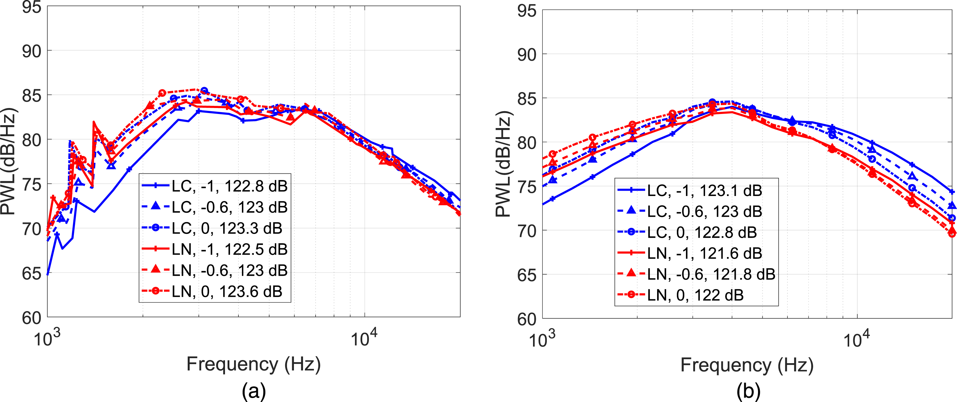
The OAPWL for LN and LC vanes are shown in Figure 19. The LN vane is only investigated up to the design location due to the simulation domain. Similar to the LC and BL vanes, both models show that the broadband OAPWL predicted using the swept LN vane is not strongly affected by the vane placement. Also Hanson’s model tends to predict lower overall sound power compared to BU-RSI. For the LC vane, the difference between the two models increases with speed, whereas the LN vane shows similar differences between the two models across the three operating conditions. OAPWL as a function of normalized FEGV placement using LC and LN vanes.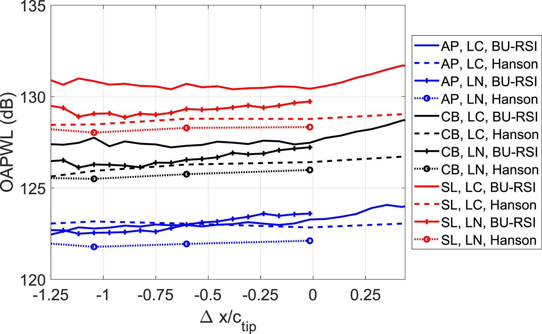
In Figure 20, the trends are compared across all three vane types at the Approach condition. Again, the BU-RSI is being compared to Hanson’s model with a Gaussian modeled wake and discriminate averaged Λ
k
. Hanson’s model shows that the BL vane case changes the most in the region Δx/c
tip
= −1.25 to 0, while BU-RSI shows that the LN vane changes the most. All of the changes however are within roughly |1 dB|. ΔOAPWL at the Approach condition for all three vane types.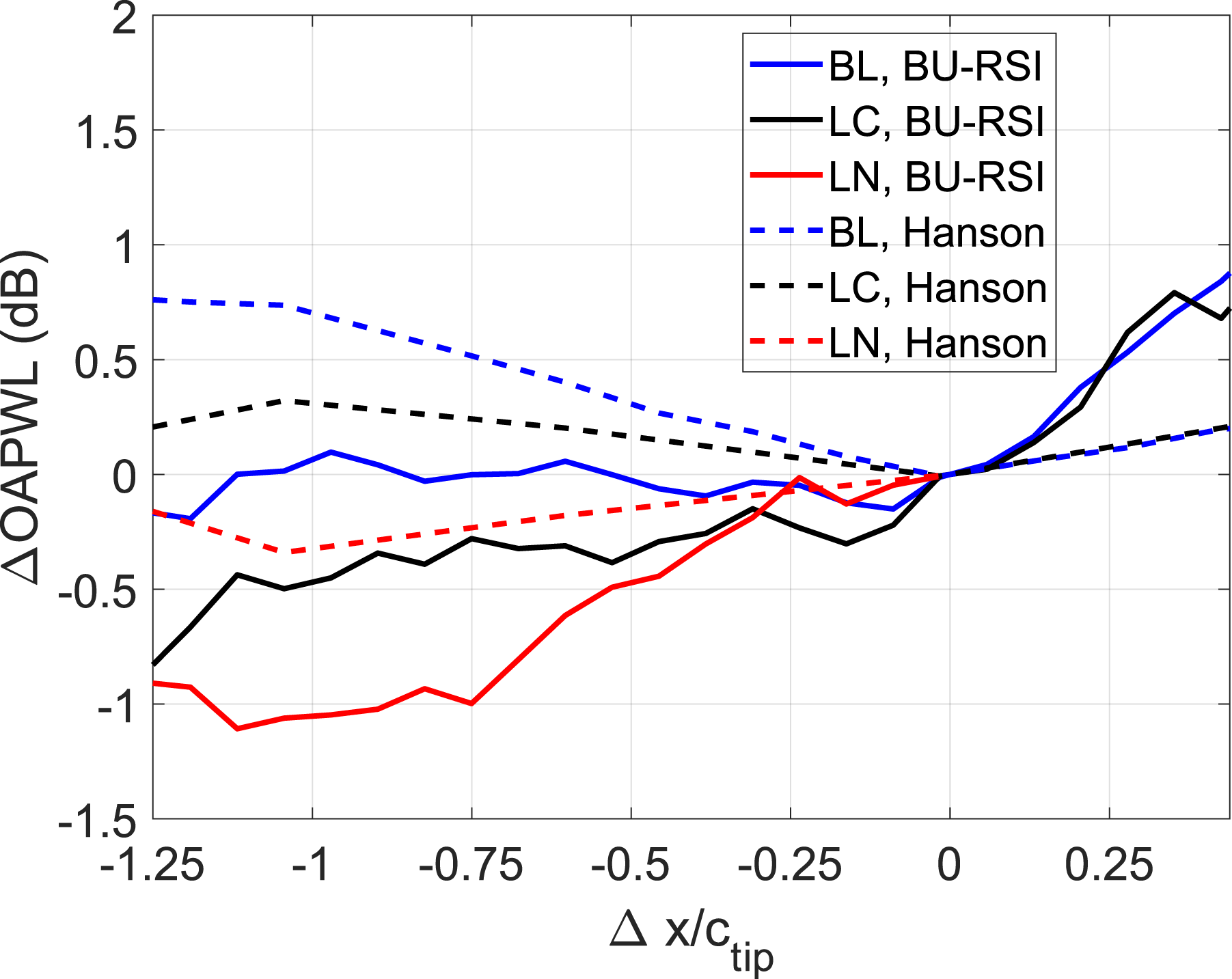
Hanson’s model shows slightly more decrease in OAPWL from Δx/c tip = −1.25 to 0, and both models show that the LC vane has slightly lower Δ in this region. The trend of the swept LN vane is quite different from the BL and LC vanes, due to the leading edge location, which extends much further downstream such that the LN vane experiences less change in turbulence length scale and more flow acceleration.
Conclusions
This paper presented a study on the effect of fan exit guide vane axial placement on the downstream propagated broadband acoustic power spectrum and OAPWL using two different low-order models (BU-RSI and Hanson). The models are examples of distinct categories of low-order methods: the BU-RSI model computes acoustic propagation in a duct via Green’s method and Hanson’s model allows free-field acoustic propagation. The analyses utilized flow inputs extracted from RANS simulations of the SDT fan. Several inflow turbulence definitions were tested, including circumferentially-averaged wake values implying a locally homogeneous wake, and a Gaussian-modeled wake using two different length scale averaging methods: fully averaged and discriminate averaged. The effect of using a RANS k − ω-based length scale and an empirical wake width-based length scale was also investigated.
The main findings are summarized here. (1) The influence of modeling inhomogeneous inflow turbulence depends on the wake width. Inhomogeneous modeling has little effect on the vane placement trend for broadband noise at the Approach condition, and up to 1 dB difference in OAPWL at the Sideline condition. (2) Turbulence length scales from both empirical wake width-based and two-equation k − ω turbulence model-based methods agree well with the experiment. However, the sound power spectrum is highly sensitive to the length scale near the shroud where the wake width-based method becomes questionable. (3) Changing vane placement tilts the sound power spectrum due to turbulence length scale evolution. Shortening the fan-FEGV gap reduces low frequency noise and increases high frequency noise. (4) The difference in broadband OAPWL due to vane placement is less than 1 dB. (5) Shifting the vane towards the direction where duct area decreases produces higher broadband noise levels. (6) Hanson’s model predicted higher sound power under 3 kHz, and lower sound power for frequencies above 3 kHz compared to BU-RSI. This leads to 2-3 dB difference in terms of OAPWL. (7) Both models showed similar trends in terms of the effect of FEGV sweep and placement. Adding sweep slightly reduced the overall broadband noise for up to 2 dB. (8) The two models showed some disagreements in terms of OAPWL for up to 1 dB for the upstream placement. Both models suggested an increase in OAPWL for the downstream placements due to the pinched duct, but Hanson’s model showed a milder increase in sound power due to flow acceleration compared to the BU-RSI model.
The findings suggest that, unlike tonal noise, which greatly decreases as the distance between the FEGV and the fan increases, the broadband noise barely changes. Depending on the case, the two low-order methods may disagree in whether the broadband noise slightly increases, remains the same, or slightly decreases, but all of the changes are within 1 dB. It is shown that placing the FEGV at a location where the duct area decreases is undesirable, as the broadband noise increases as the mean flow increases. This conclusion suggests that based solely on the broadband noise, shorter fan stage gaps can be considered without a great noise penalty.
Footnotes
Acknowledgements
This research was partially funded by the U.S. Federal Aviation Administration Office of Environment and Energy through ASCENT, the FAA Center of Excellence for Alternative Jet Fuels and the Environment, project 75 through FAA Award Number 13-C-AJFE-BU under the supervision of Christopher Dorbian. Any opinions, findings, conclusions or recommendations expressed in this material are those of the authors and do not necessarily reflect the views of the FAA. Other funding has come from RTRC and BU Mechanical Engineering Department. The development of the low-order acoustic method BU-RSI was funded through the Ohio Aerospace Institute on a grant from the AeroAcoustics Research Consortium. The authors also thank Éric Turgeon and François Bolduc-Teasdale from Optis Engineering for help in using their software OptiSound and Marlène Sanjosé for technical discussions related to the OptiSound software.
Funding
The authors disclosed receipt of the following financial support for the research, authorship, and/or publication of this article: This work was supported by the Federal Aviation Administration; 13-C-AJFE-BU.
Declaration of conflicting interests
The authors declared no potential conflicts of interest with respect to the research, authorship, and/or publication of this article.