Prediction of ducted diaphragm noise using a stochastic approach with adapted temporal filters

Abstract

The noise production by ducted single- and double-diaphragm configurations is simulated using a stochastic noise generation and radiation numerical method. The importance of modeling correctly the anisotropy and temporal de-correlation is discussed, based on numerical results obtained by large eddy simulation. A new temporal filter is proposed, designed to provide the targeted spectral decay of energy in an Eulerian reference frame. An anisotropy correction is implemented using a non-linear model. The acoustic propagation problem is solved using Lighthill’s aeroacoustic analogy with a tailored Green’s function obtained analytically. Comparison with scale--resolved data indicates that accurate far-field noise predictions are obtained for both single and double diaphragm configurations, with computational costs significantly reduced with respect to the scale-resolved approach. A grouping scheme for the noise sources based on the octree structure is introduced to minimize the memory requirements and further reduce the computational cost.

Keywords

Stochastic noise generation and radiation method aeroacoustic analogies duct acoustics tailored Green’s function large eddy simulation

Introduction

The noise generated by heating, ventilation and air conditioning (HVAC) systems is a problem encountered in many domestic and industrial applications, affecting human comfort and occupational health. With the increasing trend to use more and more electric vehicles in public and private transportation, HVAC noise problem has gained even more importance: in the absence of combustion engine noise, the noise coming from the HVAC systems simply became more audible. A significant contributor to the HVAC noise in many applications is the flow noise generated by various flow obstructions installed in the HVAC system to balance the mass flow among the branches of the ventilation network. Since the noise generation mechanism associated with the interaction of the flow with solid surfaces is rather complex, designing an HVAC system to achieve a target noise level is not possible without optimization. It is therefore essential to have a fast and reliable tool to predict flow-generated noise in ducted systems.

Methods to compute flow-induced noise commonly rely on unsteady flow data, such as large eddy simulation (LES),¹ detached eddy simulation (DES) or some of its variants.² Quite accurate noise prediction can be obtained, but the computational costs associated with such approaches do not allow the numerous runs that are necessary for numerical optimization. As a less compute intensive alternative, stochastic approaches do not explicitly resolve the unsteady Navier–Stokes equations, but are based on a generation of transient flow data satisfying statistical properties obtained by means of, for instance, Reynolds-averaged Navier–Stokes (RANS) simulations.

The use of stochastic methods to synthesize turbulence was introduced by Kraichnan³ to provide realistic boundary conditions for LES computations. Karweit et al.⁴ used this concept to develop the so-called “stochastic noise generation and radiation” (SNGR) method, where the turbulent velocity field was defined as the summation of the random Fourier modes homogeneously distributed in space. The energy level of the modes was determined using the one-dimensional von Karman-Pao energy spectrum, which is locally computed based on the mean turbulent kinetic energy and dissipation rate data obtained from a RANS solution. Bechara et al.⁵ used this approach to predict the noise generated by free turbulent flows. To introduce a temporal correlation, a band-pass filter was applied to the uncorrelated turbulent velocity data. Bailly et al.⁶ introduced the idea of convecting the synthetic field with the mean flow and providing the temporal de-correlation by adding a time- and wavenumber-dependent phase term for each Fourier mode. They implemented the method for both confined⁶ and unconfined flows.⁷ Bauer et al.⁸ applied the SGNR method to generate frozen turbulence around a flat plate to predict the trailing edge noise. Concerning the effect of the sweeping hypothesis (small eddies being carried by the most energetic eddies) on jet noise prediction,⁹ Lafitte et al.¹⁰ modified the SNGR formulation of Bailly et al.⁶ to include this effect. To introduce temporal de-correlation in SNGR method in a realistic and efficient way, Billson et al.¹¹ proposed a two-step method, where a simple convection equation was used to take into account the convection of the turbulence and the temporal de-correlation was achieved blending the convected velocity field with synthetic field at each time instant using an exponentially weighted filter. In a later work,¹² they extended this method to take the anisotropy into account.

In the present study, the SNGR approach is followed to predict the noise coming from single and double diaphragms installed in a cylindrical duct. Such configurations are frequently used in HVAC applications to balance the mass flow rate, for being very easy to manufacture and install, albeit causing significant noise. In a previous work,¹³ the authors of the present paper implemented the SNGR method of Bailly et al.,⁶ based on a three-dimensional RANS simulation, as an initial attempt to predict the noise due to ducted diaphragms. The radiation of the acoustic sources was computed using Lighthill’s analogy, implemented in a numerical acoustic solver. In parallel, Curle’s analogy¹⁴ was applied using unsteady pressure data obtained over the diaphragm surfaces by means of LES, to better understand the contribution of the diaphragm(s) to noise generation. The two numerical predictions were compared to in-duct acoustic measurements. Although the SNGR implementation showed some promising behavior, significant discrepancies remained, which were attributed to the insufficient match between the statistical properties of the RANS and LES flow fields on the one hand, and to the known numerical issues that are encountered when the Lighthill sources are located too close to the boundaries of the acoustic mesh on the other hand. To minimize those numerical errors, a tailored Green’s function was introduced in Karban et al.¹⁵ for the single and the double diaphragm cases. This approach was validated using turbulent velocity field data obtained from LES; the results were also compared with the measurements. In the present work, the same methodology is followed replacing the unsteady LES data with the synthetic turbulent velocity field obtained from the SNGR method of Billson et al.¹²

Stochastic methods rely on a statistical description of the flow field for the generation of synthetic time-resolved velocity fields. Lighthill’s approach to flow-induced noise¹⁶ indicates the importance of two-point statistics in particular. Various studies have been published on the relation between the space–time correlation functions and the noise generation in jet or shear flows.^17–20 Accordingly, stochastic noise prediction approaches are often based on the determination of the turbulent length- and time-scales from RANS k-ε or k-ω models, sometimes complemented by ad hoc calibration procedures to yield a satisfactory match with observations. This preliminary calculation often relies on an assumption of isotropic homogeneous turbulence. However, flow properties such as isotropy are strongly dependent on geometric details, making it difficult to develop a generic method applicable to a wide range of cases.

Thereto, an important objective of this work is to minimize the amount of input needed for the calibration of the length and time scales. The focus is placed on designing a new temporal filter, in which spectral decay is adjusted according to LES data to better represent the dissipation of turbulence. The effect of anisotropy is also investigated using a non-linear model for anisotropy correction. The noise prediction using the compressible LES data which was already presented in Karban et al.¹⁵ is taken as the reference data for comparison. For a reliable evaluation of the capability of the SNGR method in predicting the ducted diaphragm noise, the mean flow data were obtained averaging the LES field, eliminating errors due to discrepancies between the RANS and LES statistics. An aeroacoustic source grouping scheme, similar to the one introduced in Karban et al.,¹⁵ is implemented in the present study prior to the computation of the synthetic field using generic source terms to further reduce the memory requirements and computational cost of the acoustic propagation problem.

The organization of the paper is given as follows. The detailed description of the two ducted diaphragm cases considered is given in next section. The theory of the SNGR method implemented in this work is explained in the third section, together with the approach to compute the mean flow parameters using the LES data. The design of the new temporal filter is introduced in the fourth section and the details of the numerical set-up together with the analysis of the resulting synthetic fields are discussed in the fifth section. The far-field noise comparisons of the SNGR method against the LES results are presented in sixth section, and some final remarks about the results and the method are given in last section.

Description of the flow cases

The two flow domains corresponding to the single and double diaphragm configurations are depicted in Figure 1. The cylindrical ducted diaphragm configuration represents a toy model of an obstruction such as a valve in an HVAC system. Circular diaphragms are also found in complex duct systems with multiple side-branches, in order to balance the flow rate between the branches, alleviating the need for separate blowers. The duct diameter D is equal to 0.15 m and the thickness of the diaphragms is equal to 0.008 m. The distance between the diaphragms for the double diaphragm configuration is 2D to avoid any whistling mechanism, which was experimentally verified in Karban et al.¹³ The lengths of the inlet and the outlet sections are 6D and 9D, respectively. The blockage ratio offered by the diaphragms is equal to 0.675. The inflow velocity is 6 m/s corresponding to a Reynolds number Re = 60, 800, and the Mach number at the beginning of the (upstream) jet, where it has the highest value, is around M = 0.06.

Figure 1.

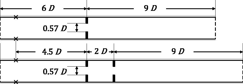
Flow domain for the single (top) and the double (bottom) diaphragm configurations. The marks × denote the listener position.

The reference flow fields for both cases have been processed from compressible LES data obtained using the AVBP solver²¹ (provided by CERFACS and EFP). It solves the Navier–Stokes equations on unstructured meshes using the Wall-Adaptive Layer Eddy (WALE) model²² for sub-grid scale modeling and the Navier–Stokes characteristic boundary conditions (NSCBC)²³ based on the so-called plane wave masking method.²⁴ The numbers of mesh elements used for the single and double diaphragm cases are 12 million and 15.5 million, respectively. The unit distance of the first element near the wall is r+ = 5 on the duct surfaces, and r+ = 1 around the edges of the diaphragm(s) in both cases. A mesh convergence analysis demonstrated that this resolution, while being generally too coarse for a proper wall-resolved LES on the duct surfaces, is sufficient in this case where the dominant sources are shed at the sharp diaphragm edge. A uniform velocity profile with magnitude 6 m/s was prescribed as the inlet boundary condition, while the pressure at the outlet was set to 101,625 Pa. The inlet velocity and the outlet pressure are corrected by subtracting the acoustic velocity and pressure obtained from the NSCBC at each time step to avoid numerical reflections. The time step of the simulation satisfied a Courant-Friedrichs-Lewy (CFL) number equal to 0.7 at maximum. The frequency range of interest is 100–6000 Hz. 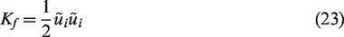The listener is located at $4.5 D$ upstream of the diaphragm, ensuring far-field conditions for the given frequency range, i.e. the evanescent waves decay out before reaching the listener point. For both single and double diaphragm configurations, the simulations have been conducted for one duct axial through-flow, proven to be sufficient for converged Fourier transform and acoustic response calculations even for the lowest frequencies of interest, and have been stored at 12,500 Hz to satisfy the Nyquist theorem. The LES data (and later the SNGR data) have been processed in segments of 150 time steps and the fast Fourier transform (FFT) of those segments was taken using 256 FFT points.

SNGR method

All the SNGR formulations in the literature are based on the representation of the turbulent velocity field as a weighted summation of Fourier modes which are randomly and homogeneously distributed in three-dimensional space as follows

u_{t} (x, t) = 2 \sum_{n =1}^{N} {\hat{u}}_{n} cos (k_{n} \cdot x + ψ_{n}) σ_{n}

(1)

where

k_{n}

is the wavevector whose magnitude gives the wavenumber and

{\hat{u}}_{n}, ψ_{n}

, and

σ_{n}

are the amplitude, phase, and unit direction of the

n th

Fourier mode, respectively.

σ_{n}

is defined on a plane normal to

k_{n}

to obtain a solenoidal velocity field (see Figure 2). To achieve homogeneous distribution of the wave vectors in three-dimensional space, the following probability density functions (PDF) are used while determining the angles

θ_{n}

and

φ_{n}

which define the orientation of

n th

the wave vector

P_{φ} = {(2 π)}^{- 1}, - π \leq φ_{n} \leq π

(2)

P_{θ} = - sin (θ_{n}) / 2, 0 \leq θ_{n} \leq π

(3)

Figure 2.

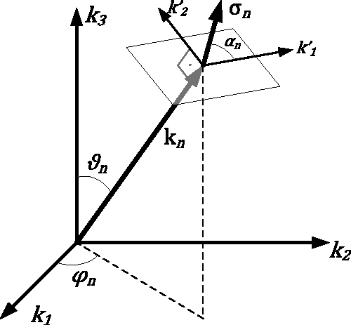
Geometric representation of a wave vector.

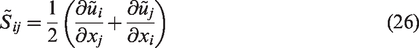
The direction of the $n th$ Fourier mode defined by the angle $α_{n}$ is expected to be randomly distributed on the plane perpendicular to the $n th$ wave vector. Therefore, the PDF corresponding to $α_{n}$ is given as follows

P_{α} = {(2 π)}^{- 1}, - π \leq α_{n} \leq π

(4)

Similarly, the phase of the $n th$ Fourier mode, $ψ_{n}$ is determined randomly with the following PDF

P_{ψ} = {(2 π)}^{- 1}, - π \leq ψ_{n} \leq π

(5)

The amplitude of the $n th$ Fourier mode is ${\hat{u}}_{n} = \sqrt{E (k_{n}) Δ k_{n}}$ , where E(k) denotes the one-dimensional von Karman-Pao energy spectrum^25,26 for isotropic turbulence given as

E (k) = \frac{4}{\sqrt{π}} \frac{Γ (17 / 6)}{Γ (1 / 3)} \frac{2 K / 3}{k_{e}} \frac{{(k / k_{e})}^{4}}{{[1 + {(k / k_{e})}^{2}]}^{17 / 6}} e^{- 2 {(\frac{k}{k_{η}})}^{2}}

(6)

and

Δ k_{n}

is the bandwidth of the

n th

wave number. In equation (6), K denotes the turbulent kinetic energy, k_e and

k_{η}

are the wavenumbers corresponding to the integral and Kolmogorov length scales, respectively. These scales are locally calculated by the following two equations

k_{η} = ϵ^{1 / 4} ν^{- 3 / 4}

(7)

k_{e} = \frac{9 π}{55} \frac{α}{Λ}

(8)

where ν, ϵ, and

Λ

correspond to the kinematic viscosity, dissipation rate, and the integral length scale, respectively. The coefficient, α is used for scaling the spectrum so that the integration of the spectrum along

(0, k)

where

k \to \infty

yields the turbulent kinetic energy. To have such an equality, α must satisfy the following, assuming Reynolds number

\to \infty

α = \frac{4}{\sqrt{π}} \frac{Γ (17 / 6)}{Γ (1 / 3)}

(9)

The integral length scale is computed by

Λ = \frac{K^{- 3 / 2}}{ϵ}

(10)

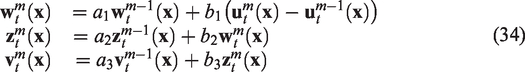
Two important physical phenomena to take into account in stochastic approaches are the convection and the temporal de-correlation of turbulence. There have been various approaches in the literature to include these effects in the resultant velocity field. Bechara et al.⁵ proposed including the convection effect by updating the position vector x in equation (1) as $x - u_{c} t$ , where $u_{c}$ is the mean convection velocity and t is the simulation time. In a later work, Bailly et al.⁶ added also a time varying phase, $ω_{n} t$ to introduce temporal de-correlation, where $ω_{n}$ denoted the angular frequency of the corresponding $n th$ mode. Investigating this approach, Omais et al.²⁷ showed that any time-dependent variable added to change the phase of the Fourier mode in equation (1) is to be uniformly distributed in space. This means that the time-dependent terms introduced for the convection and the temporal de-correlation of turbulence cause non-physical results in case of inhomogeneous turbulence.

Alternatively, Billson et al.¹¹ proposed a two-step method for the generation of synthetic turbulence to better represent the flow de-correlation in time, which is adopted in the present study. In their approach, the turbulent velocity field, $v_{t}^{m - 1} (x)$ at the time step $(m - 1)$ is convected through the convection equation

\frac{\partial (\bar{ρ} v_{t}^{m - 1})}{\partial t} + \frac{\partial (\bar{ρ u_{j}} v_{t}^{m - 1})}{\partial x_{j}} = 0

(11)

where

\bar{ρ}

and

\bar{ρ u_{j}}

correspond to the mean density and mean momentum, respectively. Then, to obtain the turbulent velocity field at time step (m), the convected velocity field is blended with the synthetic turbulent velocity fields generated at time steps (m) and

(m - 1)

using equation (1). This blending operation results an exponentially weighted temporal filter equation of Holt–Winters type^28,29

v_{t}^{m} (x) = a v_{t}^{m - 1} (x) + b (u_{t}^{m} (x) - u_{t}^{m - 1} (x))

(12)

where

a = exp (- Δ t / τ_{f})

and

b = \sqrt{(1 - a) / 2}

. The terms

Δ t

and

τ_{f}

are the time step size and the local dynamic time scale, respectively. Choosing a proper model for the time constant is crucial for accurate prediction of turbulent flow noise.³⁰ In the original work of Billson et al.,¹¹ the time constant

τ_{f}

was predicted as

τ_{f} = \frac{K}{ϵ}

(13)

The applicability of a frequency-independent time constant is to be verified for the present flow case, as the time and the length scales in turbulent flows can also be frequency dependent³¹ and the dependency of the scales on the frequency significantly affects the flow noise generation.³⁰ To examine the existence of such a dependency on the frequency in the present case, the cross-power spectral density (CPSD) of velocity has been computed at each point in the flow domain for increasing time-lag values using

Γ_{u u} (x, ω, τ_{i}) = F {u (x, t) u (x, t + τ_{i})}

(14)

where

F {\cdot}

is the discrete Fourier transform operator,

τ_{i} = i Δ τ

is the time lag at the

i th

iteration for

i = 1, 2, \dots, N

. The local Eulerian time scales are then calculated for each frequency

L_{ω} = \sum_{i = 1}^{N} Γ_{u u} (x, ω, τ_{i}) Δ τ

(15)

and normalized using

l_{ω} = \frac{L_{ω} U_{r e f}}{E {Λ}}

(16)

where U_ref is selected to be the inflow velocity and

E {Λ}

is the integral length scale averaged over the flow domain. The resulting normalized time scales at various points downstream of the diaphragm are plotted with respect to the Strouhal number,

S t = f D / U_{r e f}

in Figure 3, where U_ref is selected to be the inflow velocity.

Figure 3.

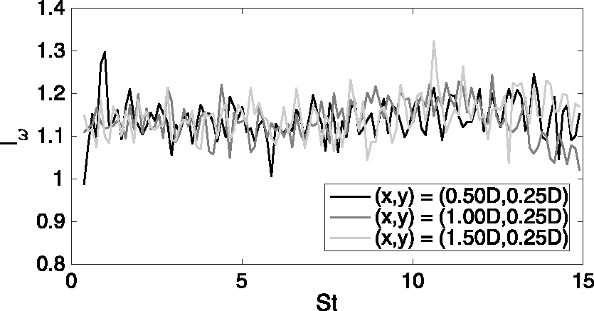
Normalized Eulerian time scales vs. Strouhal number computed at various points downstream the diaphragm for the single diaphragm case. The center of the diaphragm cross-section is taken as the origin.

As seen in the figure, no strong variation is observed for the frequency range of interest. Hence the expression used for the time scale given in equation (13) has been adopted for the present study. In the original implementation, the integral length and time scales, and the turbulent kinetic energy are tuned with some adjustment parameters. These parameters were neglected in the present study as no such tuning was conducted.

Anisotropy correction

To include the effect of anisotropy, Billson et al.¹² introduced the idea of distorting the isotropic synthetic turbulent velocity field using the Reynolds stress tensor as discussed below. The local Reynolds stress tensor, $τ = ρ u u^{⊤}$ is normalized as

a = - \frac{3}{2} \frac{τ}{\bar{ρ K}}

(17)

and is rotated to its principal axes to yield

a^{*} = R^{⊤} a R

(18)

Since a is symmetric, the above rotation can be achieved by finding the eigenvalues, h_i and the eigenvectors, $h_{i}$ of a such that $a^{*} = d i a g {h_{i}}$ and $R = [h_{1} \dots h_{z}]$ where z is the rank of a.

Anisotropy can be added to the isotropic turbulent velocity field, which is calculated using equation (1), by (i) rotating all the vectors to the principal axes (multiplying by $R^{⊤}$ ), (ii) scaling the Fourier summation with $a^{*}^{1 / 2}$ , and (iii) rotating the resulting vector field back to the original coordinate system (multiplying by $R$ ). To retain the divergence-free characteristic of the turbulent velocity field, the wave vector k is to be scaled with $a^{*}^{- 1 / 2}$ . It was shown in Billson et al.¹² that the stress tensor calculated from the resulting turbulent velocity field satisfies the given stress tensor $τ$ . There are various models in the literature for predicting the anisotropy from the mean flow velocity data. In Billson et al.,¹² a linear eddy viscosity model has been used to predict the anisotropy. Omais et al.²⁷ showed that use of a non-linear Reynolds stress model (RSM) significantly improves the prediction of the anisotropy, and so does the accuracy of the SNGR method. Following their approach, the non-linear RSM introduced by Shih et al.³² is implemented in the present study. The RSM is given by

\bar{u_{i} u_{j}} = \frac{2}{3} K δ_{i j} - C_{μ} \frac{K^{2}}{ϵ} 2 S_{i j}^{*} + 2 C_{2} \frac{K^{3}}{ϵ^{2}} (- S_{i k}^{*} Ω_{k j}^{*} + Ω_{i k}^{*} S_{k j}^{*})

(19)

where

S_{i j}^{*}

is the traceless strain tensor given as

S_{i j}^{*} = \frac{1}{2} (\frac{\partial {\bar{U}}_{i}}{\partial x_{j}} + \frac{\partial {\bar{U}}_{j}}{\partial x_{i}}) - \frac{1}{3} \frac{\partial {\bar{U}}_{k}}{\partial x_{k}} δ_{i j}

(20)

and

Ω_{i j}^{*}

is the vorticity tensor

Ω_{i j}^{*} = \frac{1}{2} (\frac{\partial {\bar{U}}_{i}}{\partial x_{j}} - \frac{\partial {\bar{U}}_{j}}{\partial x_{i}})

(21)

with

{\bar{U}}_{i}

representing the mean flow velocity. To satisfy the realizability in any flow condition, Shih et al.³² defined the coefficients

C_{μ}

and C₂ in equation (19) according to the rate of deformation and the rate of rotation of the mean flow

C_{μ} = \frac{1}{A_{0} + A_{s}^{*} \frac{U^{*} k}{ϵ}}, C_{2} = \frac{\sqrt{1 - 9 C_{μ}^{2} (\frac{S^{*} k}{ϵ})}}{C_{0} + 6 \frac{S^{*} k}{ϵ} \frac{Ω^{*} k}{ϵ}}

(22)

where

A_{0} = 6.5, C_{0} = 1, S^{*} = \sqrt{S_{i j}^{*} S_{j i}^{*}}, Ω^{*} = \sqrt{Ω_{i j}^{*} Ω_{j i}^{*}}, A_{s}^{*} = \sqrt{6} cos (\frac{1}{3} arccos (\sqrt{6} W^{*})), U^{*} = \sqrt{S_{i j}^{*} S_{i j}^{*} + Ω_{i j}^{*} Ω_{i j}^{*}}, and W^{*} = \frac{S_{i j}^{*} S_{j k}^{*} S_{k i}^{*}}{{(S^{*})}^{3}} .

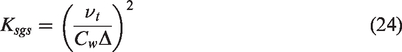
Computing the mean flow parameters using the LES data

The mean flow field required as input in the above analysis is usually provided by a RANS simulation in order to minimize the computational costs. However, the present study being aimed at evaluating the accuracy of the SNGR synthesis by comparing the predicted acoustic field with the prediction obtained from unsteady LES data, the mean flow statistics are here calculated from the LES data for the sake of avoiding ambiguities that could result from different RANS and LES statistics.

To obtain the turbulent kinetic energy and the dissipation rate from the LES, the conservation equation for the filtered turbulent kinetic energy has been used. Any flow variable in an LES model can be written as the summation of the filtered and the sub-grid scale parts. For the turbulent kinetic energy K, the filtered part, K_f can be directly computed using the filtered turbulent velocity field data, ${\tilde{u}}_{i}$

K_{f} = \frac{1}{2} {\tilde{u}}_{i} {\tilde{u}}_{i}

(23)

The modeled turbulent eddy viscosity $ν_{t}$ is an output of the solver. The sub-grid scale part of the turbulent kinetic energy, K_sgs can be predicted using

K_{s g s} = {(\frac{ν_{t}}{C_{w} Δ})}^{2}

(24)

where C_w is the model constant (=0.57 for the WALE model) and the

Δ

is the characteristic filter size computed as the cubic root of the volume of the corresponding mesh element. For the prediction of the dissipation rate, the conservation equation for the filtered kinetic energy, K_f as given in Pope’s book³³ is considered

\frac{\tilde{D} K_{f}}{\tilde{D} t} - \frac{\partial}{\partial x_{i}} [{\tilde{u}}_{j} (2 ν {\tilde{S}}_{i j} - τ_{i j}^{r} - \frac{\tilde{p}}{ρ} δ_{i j})] = - ϵ_{f} - P_{r}

(25)

where

{\tilde{S}}_{i j} = \frac{1}{2} (\frac{\partial {\tilde{u}}_{i}}{\partial x_{j}} + \frac{\partial {\tilde{u}}_{j}}{\partial x_{i}})

(26)

represents the filtered stress tensor, and

τ_{i j}^{r}

corresponds to the residual stress computed using the linear eddy viscosity model

τ_{i j}^{r} = - 2 ν_{t} {\tilde{S}}_{i j}

(27)

The left hand side of equation (25) represents the transport of the filtered energy, while the right hand side is related to viscous dissipation ( $ϵ_{f}$ being the viscous dissipation of the filtered field) and rate of the transfer of the kinetic energy to the sub-grid scale ( $P_{r}$ ). Assuming a temporarily stationary flow, i.e. the net production of the kinetic energy equals zero, the total dissipation rate, ϵ in the flow field can be found by summing these two terms

ϵ = ϵ_{f} + P_{r}

(28)

where

ϵ_{f} \equiv ν {\tilde{S}}_{i j} {\tilde{S}}_{i j}

(29)

P_{r} \equiv - τ_{i j}^{r} {\tilde{S}}_{i j}

(30)

A new temporal filter

The energy spectra of the noise sources observed in an Eulerian frame within a flow are affected by the sweeping of turbulence.¹⁸ This is achieved with the convection operation in the present SNGR implementation. In flow regions with strong convection, the noise sources are characterized by the spatially generated synthetic velocity field. However, for the flow regions where the mean convection velocity is close to zero, such as the recirculation zone(s) downstream of the diaphragm(s) shown in Figure 4, the temporal de-correlation obtained by the filter given in equation (12) becomes also effective in defining the turbulent fluctuations in an Eulerian frame. Despite their relatively low turbulence intensity, the acoustic sources contained within those regions may still have significant contribution, since their radiation efficiency is enhanced by the proximity of the diaphragm(s). Hence, it is important for the spectral decay of the filter to match the LES value for those regions. For the single diaphragm configuration, the energy spectra of the velocity data at randomly selected various points within the separation zone are calculated using the LES data and depicted in Figure 5. Since the LES data includes compressibility effects, peaks in the spectra are observed at the cut-on frequencies, where new acoustic modes become propagative. It is seen that for the frequency range where the shape of the spectrum is not dominated by acoustic mode cut-on, the spectral decay can be approximated by a −4.5 slope. This spectral decay being much steeper than −5/3, it can be inferred that the energy spectrum corresponding to the frequency range of interest exhibits more dissipation than in isotropic homogeneous turbulence. Similar values for the spectral decay in the dissipative range were reported in various experimental studies investigating the energy spectrum in pipe flows.^34–36 The Reynolds number of the flow investigated in the present study is $R e_{D} = U D / ν ≅$ 64,000. In the work of Torbergsen and Krogstad,³⁴ the closest experimental case available for comparison with $R e_{D} =$ 70,000, the computed spectral decay was −4.2, fairly close to the value predicted from the present LES.

Figure 4.

The mean u-velocity field for the single diaphragm case. The white-dashed line denotes the separation zone downstream of the diaphragm.

Figure 5.

Energy spectrum of the u-velocity at various points in the separation zone.

The logarithmic slope of the spectrum of the temporal filter given in equation (12) can be calculated by taking the Fourier transform

V_{ω} = a V_{ω} e^{- \frac{2 π ω}{N}} + b (U_{ω} + U_{ω} e^{- \frac{2 π ω}{N}})

(31)

where

V_{ω}

and

U_{ω}

are the Fourier Transform of v and

u

, respectively, and N is the number of the discrete time instants. Since the synthetic velocity field

u (x)

is uncorrelated in time, its Fourier transform yields a constant, γ. Reorganizing equation (31) and taking the logarithm, one obtains

log V_{ω} = log b +log γ +log (1 + e^{- \frac{2 π ω}{N}}) - log (1 - a e^{- \frac{2 π ω}{N}})

(32)

Taking the derivative of equation (32) with respect to $\log ω$ and multiplying by 2 yields the logarithmic slope of the energy spectrum of the temporal filter

slope = - \frac{4 π ω}{N} e^{- \frac{2 π ω}{N}} (\frac{1}{1 + e^{- 2 π ω / N}} + a \frac{1}{1 - e^{- 2 π ω / N}})

(33)

The slope given in equation (33) is only dependent on the coefficient a, which is a function of the time step $Δ t$ , and the time constant $τ_{f}$ , neither of which are suitable for freely adjusting the slope of the filter. Given a time step satisfying the ratio, $Δ t / τ_{f} = 0.0001$ , which yields a CFL value much smaller than the limit for numerical stability, the resulting slope of the spectrum in the frequency range of interest is almost constant and approximately equal to −2; while using a bigger time step makes the slope even closer to zero. This analysis implies that using the filter given in equation (12), it is not possible to obtain a velocity field with an energy spectrum matching the LES flow field. To overcome this issue, a cascaded temporal filter is proposed in the present study as follows

\begin{matrix} w_{t}^{m} (x) = a_{1} w_{t}^{m - 1} (x) + b_{1} (u_{t}^{m} (x) - u_{t}^{m - 1} (x)) \\ z_{t}^{m} (x) = a_{2} z_{t}^{m - 1} (x) + b_{2} w_{t}^{m} (x) \\ v_{t}^{m} (x) = a_{3} v_{t}^{m - 1} (x) + b_{3} z_{t}^{m} (x) \end{matrix}

(34)

where w and z are auxiliary variables, a₁ and a₂ are free parameters used for tuning the slope of the resulting filter spectrum,

b_{1} = \sqrt{(1 - a_{1}) / 2}, b_{2} = \sqrt{(1 - a_{2})}, a_{3} = exp (- Δ t / τ_{f})

, and

b_{3} = \sqrt{(1 - a_{1})} / σ

. The correction factor, σ is added to ensure that the standard deviations of v and

u

are equal. To tune the parameters, a₁ and a₂, a random series

u

with constant spectrum is used. Setting

a_{1} = 0.98

and

a_{2} = 0.7

, the logarithmic slope of the filter spectrum over the domain of interest for the single diaphragm case lies between −4.42 and −4.51, with an average equal to −4.50. The corresponding correction factor σ is numerically computed to be 8.26 by taking the ratio of the standard deviation of v to that of

u

Once the turbulent velocity field is generated, the acoustic sources corresponding to this field and the noise generated by these sources are computed using Ligthill’s analogy¹⁶ and tailored Green’s function approach. The details can be found in Appendix 1.

Numerical setup and synthetic flow field

The mesh used for the SNGR method has to be fine enough to minimize the numerical dissipation when solving the convection equation. The SNGR mesh has been determined based on the average cell size of the LES mesh taken as reference. For both single and double diaphragm configurations, the upstream boundary of the SNGR domain has been set matching with the downstream face of the (upstream) diaphragm. Such a boundary is selected owing to the very low levels of turbulence intensity that are ingested through the upstream diaphragm, in comparison with the turbulence that develops in the downstream jet shear layer. Meshes of 1.67 × 10⁶ and 2.56 × 10⁶ elements have been created for the single and double diaphragm cases, respectively, without any particular refinement for the boundary layers. To decrease memory and computational costs for the acoustic calculations, a grouping scheme detailed in Appendix 2 has been introduced. Both the inflow and outflow boundary conditions for the turbulent velocity field have been set to 0 m/s. A buffer layer of length 2D has been applied to the downstream end of the domain to avoid spurious noise generation, where the synthetic source data are weighted by a semi-Hanning decaying window function. No buffer layer is required for the inlet, as the turbulence intensity at the upstream interface of the (upstream) diaphragm is already very close to zero.

The convection equation has been solved using a forward-time forward-space (FTFS) explicit scheme with a time step of 2 × 10⁻⁵ s. The maximum CFL number with the given mesh and time step is 0.75, below the stability limit of 1 for the selected numerical scheme. The wavenumber range has been determined through a convergence analysis. The lower bound has been taken as 0.1 min(k_e) where the minimum of the k_e-distribution within the domain of interest is calculated to be of order 10 m⁻¹ using equation (8) for both configurations. Acoustic convergence has been achieved with the upper bound of k_e set to 200 and 500 m⁻¹, and the number of wavenumbers equals 50 and 125 for the single and double diaphragm configurations, respectively.

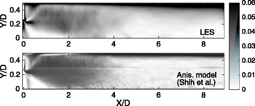
The anisotropy model investigated in the present study is compared with the anisotropy data computed from LES. The approach proposed by Lumley and Newman³⁷ has been adopted thereto. In their approach, the relation between the two invariants $I I = - a_{i j} a_{j i} / 2$ and $I I I = det (a_{i j})$ , with $a_{i j} = τ_{i j} / 2 K - 1 / 3$ , is used for determining the characteristics of the turbulence. $I I = I I I = 0$ indicates isotropic turbulence, while $I I >$ 0 and $I I I ≅$ 0 indicate two-component axisymmetric turbulence. In the present SNGR data, the invariant III is seen to be very close to zero for the entire flow domain of interest for both single and double diaphragm cases. Hence, the comparisons between the anisotropy models and the LES data are made regarding the invariant, II. In Figure 6, the II-distribution obtained from the anisotropy model and the LES data are plotted for the single diaphragm case.

Figure 6.

Comparison of the anisotropy tensor invariant, II for the single diaphragm case.

The anisotropy model is seen to underpredict the anisotropy at the onset of the jet region and in the boundary layer on the diaphragm and duct surfaces. Besides, an overprediction is observed at the tip of the jet cone at $x / D = 2$ . However, the aeroacoustic sources contained in these regions are not strong, and little effect on the noise generation is expected due to such a discrepancy. For the shear zone, the anisotropy prediction by the model is in good agreement with the LES data with a slight overprediction until $x / D = 3.5$ .

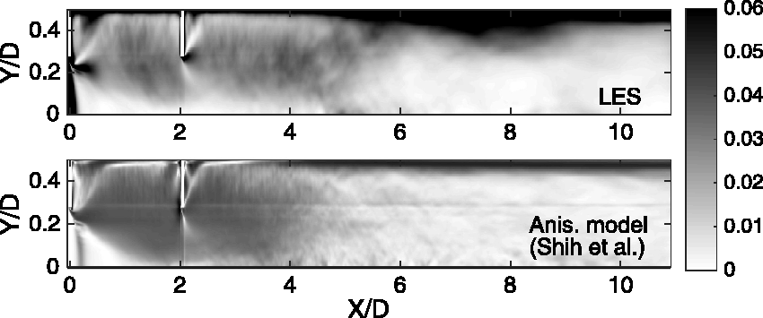
More severe discrepancies are observed in the anisotropy prediction in the tandem diaphragms case depicted in Figure 7. Once again, the anisoptropy at the onset of the jet region at $x / D = 0$ and in the boundary layer around the duct surface is underpredicted by the model. Besides, the model is observed to overpredict the anisotropy in the regions close to the opening of the downstream diaphragm. Contrary to the underpredicted parts, the flow region around the downstream diaphragm is known to be effective in noise generation. Therefore, an effect in the resulting noise prediction is expected due to this discrepancy. For the rest of the domain, the model can be considered to yield an accurate anisotropy distribution again with a slight overprediction.

Figure 7.

Comparison of the anisotropy tensor invariant, II for the double diaphragm case.

The comparison of the computational costs per CPU of a converged simulation obtained by the isotropic and anisotropic implementations of the SNGR method against the LES is given in Table 1.

Table 1.

The CPU time required per time step for the SNGR method and the LES.

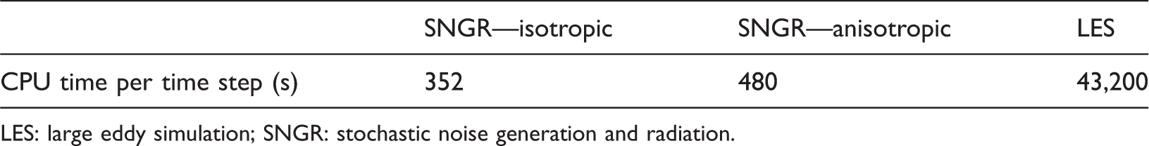
	SNGR—isotropic	SNGR—anisotropic	LES
CPU time per time step (s)	352	480	43,200

LES: large eddy simulation; SNGR: stochastic noise generation and radiation.

Comparison between acoustic predictions obtained from SNGR and LES data

The effect of the anisotropy correction developed in “Anisotropy correction” section is first evaluated, then the effect of the temporal filter proposed in “A new temporal filter” section is discussed.

Effect of the anisotropy correction

A comparison of the acoustic responses obtained from the SNGR method with and without the anisotropy correction, and from the LES data, is given in Figure 8. Using the proposed temporal filter and the non-linear anisotropy model, a very good match between the SNGR- and LES-based predictions is observed for the single diaphragm case. In contrast, an overestimation of 20 dB, about constant over the full frequency range, is obtained without the anisotropy correction. That correction consists in reorienting and scaling the velocity vectors to meet the targeted axisymmetric anisotropic character, without changing the invariants of Lighthill’s stress tensor. It can therefore be expected that the anisotropic flow field generates less noise than the isotropic one, as the correction reduces the amplitude of the off-diagonal elements of the Lighthill’s stress tensor.

Figure 8.

Far-field noise comparison of the SNGR implementations with or without anisotropy correction vs. LES in the single diaphragm case.

For the double diaphragm configuration, the effect of the anisotropy correction is seen in Figure 9 to depend on the frequency. Surprisingly, it improves the match with the LES-based prediction in the high-frequency range (above 3 kHz), but degrades the agreement in the low-frequency range (below 400 Hz). A possible reason for such a discrepancy is explained as follows. The noise generated by the sources contained in a cylindrical zone which is 0.6D in both diameter and length, and centered around the downstream diaphragm is compared to noise generated by the rest of the sources in Figure 10. It is seen that the depicted zone is mainly responsible for noise generation below 400 Hz. As mentioned above, the non-linear eddy viscosity model used in the present study overpredicts the anisotropy in this region. The anisotropy correction redistributes the energy in $x -, y -$ , and $z -$ directions which reaches its maximum in case of isotropy. Therefore, an overprediction of anisotropy causes a drop in source strength, yielding such a discrepancy in the noise levels below 400 Hz.

Figure 9.

Far-field noise comparison of the anisotropic (a) and the isotropic (b) SNGR implementations vs. LES in the double diaphragm case.

Figure 10.

The zone defined around the downstream diaphragm (a) and comparison of the noise generated by this region to that of the rest of the sources (b).

Effect of the temporal filter

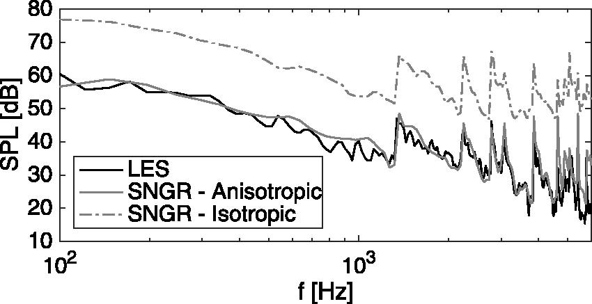
It was mentioned in the fourth section that the temporal filter used in the SNGR method is expected to have a significant effect on the noise prediction for the single diaphragm case, due to possible acoustic contribution of the flow regions with almost zero convection velocity. To see this effect, the noise prediction by the SNGR method with the cascaded temporal filter is compared to that of the original method of Billson et al. in Figure 11. The anisotropy correction is applied for both implementations. As the original temporal filter yields a shallower spectrum, a similar behavior in the resulting acoustic response is observed. It is seen in Figure 11 that the SNGR method of Billson et al. underestimates the far-field noise for frequencies lower than 1300 Hz, while an overestimation is obtained for higher frequencies.

Figure 11.

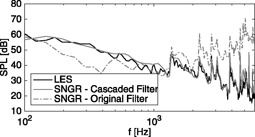
Far-field noise comparison of the SNGR implementations with different temporal filters vs. LES in the single diaphragm case.

A similar conclusion is reached for the double diaphragm case as shown in Figure 12, although the effect is less pronounced. A possible reason is that the convection velocities of the dominant noise sources are larger for the double diaphragm case than for the single diaphragm case. Hence the temporal de-correlation effect is possibly less important compared with the convective effect.

Figure 12.

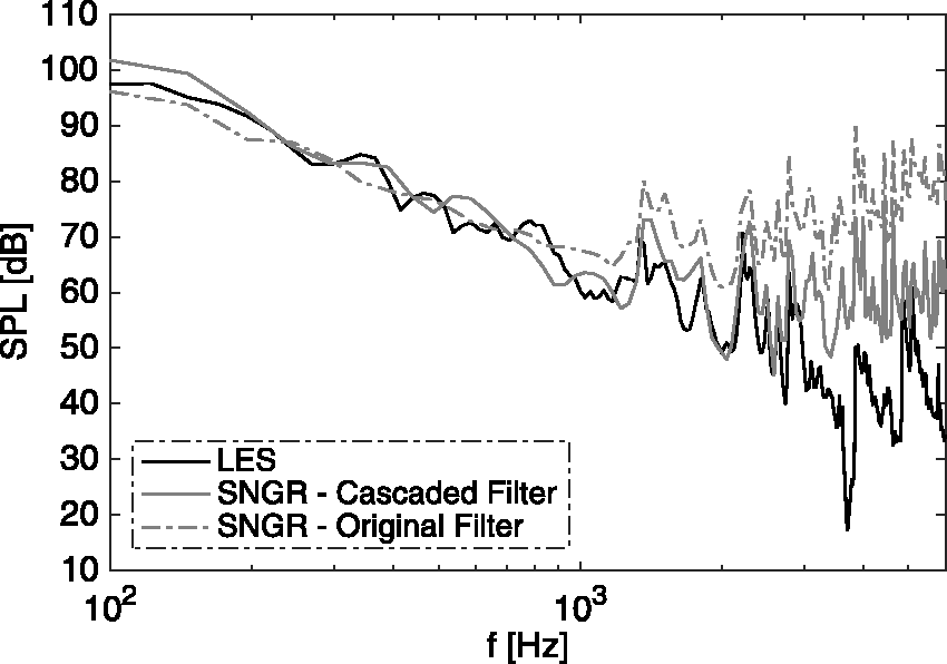
Far-field noise comparison of the SNGR implementations with different temporal filters vs. LES in the double diaphragm case.

Conclusions

The applicability of the SNGR method for the prediction of the noise emitted by single and double ducted diaphragms has been investigated. An analytical solution has been used for the propagation problem in order to avoid the effect of numerical propagation errors and focus the analysis on the accuracy of the source reconstruction. The required flow data have been obtained from LES statistics. A cascaded filter has been proposed, which was shown to yield a better match of the turbulence spectral decay with the LES data, than using the previously published temporal filter. An anisotropy correction has been implemented as well, which was shown to have a significant effect on the space–time correlation of the synthesized flow field. Lighthill’s aeroacoustic analogy has been used for computing the noise sources, and the propagation problem has been solved using a tailored Green’s function for ducted diaphragms. A significant reduction of the memory requirement and CPU time has been attained by applying a grouping scheme that was automatically optimized on the basis of dummy source data, and which should therefore not depend on the specific source data used in later calculations. This has been verified using the SNGR dataset. The noise generated by the ducted diaphragm(s) was proven to be quite accurately predicted through comparison with the LES-based result, provided that an accurate anisotropy model and a temporal filter with the correct spectral decay are applied. In particular, the benefit of introducing an anisotropy correction was quite clear for the single diaphragm case, but was shown to depend on the frequency range for the double diaphragm configuration. The good match between the SNGR and the LES results, where the CPU cost of the SNGR approach was about 1/50th of the LES CPU cost, indicates that such stochastic methods are a viable option for this category of flows and could be used for optimization purposes.

Footnotes

Declaration of conflicting interests

The author(s) declared no potential conflicts of interest with respect to the research, authorship, and/or publication of this article.

Funding

The author(s) disclosed receipt of the following financial support for the research, authorship, and/or publication of this article: the Marie Curie People program FlowAirS (ITN—project number: 289352) of the European Commission.

Appendix 1

References

Gloerfelt

Lafon

Direct computation of the noise induced by a turbulent flow through a diaphragm in a duct at low Mach number. Comput Fluids 2008; 37: 388–401.

Shur

Spalart

Strelets

et al . A hybrid RANS-LES approach with delayed-DES and wall-modelled LES capabilities. Int J Heat Fluid Flow 2008; 29: 1638–1649.

Kraichnan

RH.

Diffusion by a random velocity field. Phys Fluids 1970; 13: 22–31.

Karweit

Blanc-Benon

Juvé

et al . Simulation of the propagation of an acoustic wave through a turbulent velocity field: A study of phase variance. J Acoust Soc Am 1991; 89: 52–62.

Bechara

Bailly

Lafon

et al . Stochastic approach to noise modeling for free turbulent flows. AIAA J 1994; 32: 455–463.

Bailly

Lafon

Candel

Computation of noise generation and propagation for free and confined turbulent flows. In: AIAA and CEAS, Aeroacoustics Conference, 6-8 May 1996, 2nd, State College, PA, USA. AIAA.

Bailly

Juve

A stochastic approach to compute subsonic noise using linearized Euler’s equations. In: 5th AIAA/CEAS aeroacoustics conference and exhibit. 10-12 May 1999, Bellevue, USA, AIAA.

Bauer

Zeibig

Költzschc

Application of the SNGR-model to compute trailing edge noise. Dresden University of Technology, Germany, 2006.

Rubinstein

Zhou

The frequency spectrum of sound radiated by isotropic turbulence. Phys Lett A 2000; 267: 379–383.

10.

Lafitte

Garrec

Laurendeau

et al . A study based on the sweeping hypothesis to generate stochastic turbulence. In: 17th AIAA/CEAS aeroacoustics conference. Portland, USA, 2011. AIAA.

11.

Billson

Eriksson

Davidson

Jet noise modeling using synthetic anisotropic turbulence. In: 10th AIAA/CEAS aeroacoustics conference, 10-12 May, 2004, Manchester, Great Britain. Manchester: AIAA.

12.

Billson

Eriksson

Davidson

et al . Modeling of synthesized anisotropic turbulence and its sound emission. In: 10th AIAA/CEAS aeroacoustics conference, 10-12 May, 2004, Manchester, Great Britain. Manchester: AIAA.

13.

Karban

Ogus

Kucukcoskun

et al . Noise produced by a tandem diaphragm: experimental and numerical investigations. In: 20th AIAA/CEAS aeroacoustics conference, 16-20 June, 2014, Atlanta, GA. Atlanta: AIAA

14.

Curle

The influence of solid boundaries upon aerodynamic sound. Proc R Soc A 1955; 231: 505–514.

15.

Karban

Schram

Sovardi

et al . Tailored Green’s functions for the prediction of the noise generated by single and tandem diaphragms in a circular duct. Acta Acust Acust 2016; 102: 779–792.

16.

Lighthill

MJ.

On sound generated aerodynamically. I. General theory. Proc R Soc A 1952; 211: 564–587.

17.

Lilley

GM.

The radiated noise from isotropic turbulence. Theor Comput Fluid Dyn 1994; 6: 281–301.

18.

Rubinstein

Zhou

Time correlations and the frequency spectrum of sound radiated by turbulent flows. Institute for Computer Applications in Science and Engineering (ICASE), 1997.

19.

Ribner

HS.

Quadrupole correlations governing the pattern of jet noise. J Fluid Mech 1969; 38: 1.

20.

Lynch

Blake

Mueller

TJ.

Turbulence correlation length-scale relationships for the prediction of aeroacoustic response. AIAA J 2005; 43: 1187–1197.

21.

Sengissen

Caruelle

Souchotte

et al . LES of noise induced by flow through a double diaphragm system. In: 15th AIAA/CEAS aeroacoustics conference, 11-13 May, 2009. Miami: AIAA.

22.

Nicoud

Ducros

Subgrid-scale stress modelling based on the square of the velocity gradient tensor. Flow Turb Combust 1999; 62: 183–200.

23.

Poinsot

Lelef

SK.

Boundary conditions for direct simulations of compressible viscous flows. J Comput Phys 1992; 101: 104–129.

24.

Polifke

Wall

Moin

Partially reflecting and non-reflecting boundary conditions for simulation of compressible viscous flow. J Comput Phys 2006; 213: 437–449.

25.

von Kármán

Progress in the statistical theory of turbulence. Proc Natl Acad Sci U S A 1948; 34: 530–539.

26.

Pao

YH.

Structure of turbulent velocity and scalar fields at large wavenumbers. Phys Fluids 1965; 8: 1063.

27.

Omais

Caruelle

Redonnet

et al. Jet noise prediction using RANS CFD input. In: 14th AIAA/CEAS aeroacoustics conference, 11-13 May, 2008. Vancouver: AIAA.

28.

Holt

CC.

Forecasting seasonals and trends by exponentially weighted moving averages. Int J Forecasting 2004; 20: 5–10.

29.

Winters

PR.

Forecasting sales by exponentially weighted moving averages. Manage Sci 1960; 6: 324–342.

30.

Azarpeyvand

Self

RH.

Improved jet noise modeling using a new time-scale. J Acoust Soc Am 2009; 126: 1015–1025.

31.

Harper-Bourne

Jet near-field noise prediction. In: 5th AIAA/CEAS aeroacoustics conference and exhibit, Bellevue, USA, 1999. AIAA.

32.

Shih

Zhu

Lumley

JL.

A new Reynolds stress algebraic equation model. Comp Methods Appl Mech Eng 1995; 125: 287–302.

33.

Pope

SB.

Turbulent flows. 1st ed. Cambridge / New York, NY: Cambridge University Press, 2000.

34.

Torbergsen

Krogstad

Axisymmetric contraction of fully developed pipe flow. In: Proceedings of the 13th Australasian fluid mechanics conference. Vol. 1, 13-18 December 1998, Melbourne, Australia, pp.659–662.

35.

Zuniga Zamalloa

Experiments on turbulent flows in rough pipes: spectral scaling laws and the spectral link. Dissertation. University of Illinois at Urbana-Champaign, USA, 2012.

36.

Rosenberg

Hultmark

Vallikivi

et al . Turbulence spectra in smooth- and rough-wall pipe flow at extreme Reynolds numbers. J Fluid Mech 2013; 731: 46–63.

37.

Lumley

Newman

The return to isotropy of homogeneous turbulence. J Fluid Mech 2001; 82: 161–178.

38.

Rienstra

Hirschberg

An introduction to acoustics. Eindhoven: Eindhoven University of Technology, 2001.