
Abstract
The Ffowcs Williams–Hawkings equation is widely used in computational aeroacoustics to post-process unsteady simulations and provide the sound at distances beyond the accurate range of the grid. It distinguishes the monopole/dipole contributions from solid surfaces Σ and that from quadrupoles present in the volume of the fluid. Curle showed that at low Mach numbers, the solid-surface terms are stronger than the volume term. Very few studies have included the volume term itself, but many have used a permeable Ffowcs Williams–Hawkings surface Σ, which in principle surrounds the quadrupoles, giving valid results independent of Mach number; in reality for external flows, the surface cannot surround all the quadrupoles. However, in spite of doubts over the solid-surface approach even at low Mach numbers, it is widely used because of its simplicity and the difficulties associated with turbulence crossing the permeable surface. We consider Mach numbers M up to 0.25, which challenges approximations based on the property that “M ≪1.” An additional attraction of the solid-surface approach is the idea of identifying the “true” source of the sound by computing separately the Ffowcs Williams–Hawkings integrals for different components. We wish to determine whether this “self-evident” argument gives an effective approach, and in general to assess Curle’s approximations, using a sphere-dipole problem and three model problems related to landing-gear noise, namely an isolated rectangular body, a fuselage with a cavity, and one with a bluff body under it. One key test is the shielding of sound toward various directions; any approach that misses this shielding is suspect. The overall conclusion is, again, that Curle’s approximations succeed in some cases but are quite inaccurate in the audible range for an airliner in approach and for high-speed trains, and also that separating the components’ contributions is often misleading. In contrast we verify that, for our model problems and with adequate grid resolution and surface placement, the permeable-surface results are as accurate as the simulation itself is, irrespective of distance, direction, or Mach number.
Keywords
Introduction
Overview and Ffowcs Williams–Hawkings (FWH) formula
Our purpose is an improved understanding based on quantitative results of the issues covered in a primarily theoretical paper by one of the present authors on Acoustic Analogies, 1 hereafter JSV13 (with equation numbers such as JSV13-6). Its motivation was to clarify the community’s thinking and reporting for aerodynamic noise at low but industrially relevant Mach numbers such as 0.25, and an outcome was a challenge to some of Curle’s arguments, 2 which very much guide the interpretation of many results in this field. For instance, Curle’s statement that “quadrupole sound” scales with M8 while “dipole noise” scales with M6 was shown to be incorrect (there is a cross-term of order M7 in JSV13-16, and thus the approximation is of lower order than claimed, namely M instead of M2, which is a potent difference when M = 0.25). Yet, in the literature, the attraction of the M6 law is powerful. A practical consideration when conducting simulations, also related to Curle’s theories, is the choice between solid and permeable Ffowcs Williams–Hawkings surfaces, 3 which we discussed at length in JSV13, in Spalart et al., 4 and other papers. However, no clear guidelines on this choice are yet available in the literature.
Below we present a literature survey starting in 2013 and weight it toward 2017 and 2018, much of it based on the LAGOON model, 5 hoping this sums up the state of the art.
For reference, we present the FWH formula as we generally use it, in its far-field approximation, although a near-field version will also be used

Here,
Curle
2
correctly argued that, for aerodynamic sound at low Mach numbers, the volume term, the first one on the right-hand-side of equation (1), is of order M4, whereas the other two if evaluated on the solid surface are of order M3. He failed to recognize the cross-term of order M7 which appears when forming the intensity
Permeable surfaces and end-caps
A known issue with permeable Σ surfaces is that, for external flows, the turbulence and therefore the quadrupoles in the wake of the body inevitably cross the surface, thus negating the assumption that Σ “surrounds all the turbulence” so that the volume integral can be omitted with rigor. To combat this error, the simulation grid can be extended, but not with a resolution fine enough to sustain the turbulent eddies to the same standards as in the near-field; this has been called the “Departure Region,” as opposed to the “Focus Region.” 6 The simulation gradually removes the small-scale kinetic energy (faster than physical dissipation does, unless the Reynolds number is low), either via a subgrid-scale model, or numerical dissipation brought about by upwind-differencing or filtering. In either case, these are substantial viscous-like effects which to be rigorous would be added to the quadrupole tensor; this is far from simple and has not been done. We know of no rigorous estimate of how close to the body it is tolerable to initiate “departure-region errors.” The danger of stretching the Σ surface far downstream is of calculating “the accurate integral for turbulence that has become inaccurate,” due to numerical dissipation.
Somehow, the spurious sound caused by this “hydrodynamic” effect is often stronger for upstream observers and at low frequencies. Quite a few remedies have been proposed, which allow weakening the spurious sound. A common one is to omit the integral on the downstream “end-cap,” i.e. to use “open” control surfaces. Another is to extend the surface so far that the turbulence has essentially decayed, a decay possibly forced by the inevitable coarsening of the grid as explained above. Along with this, some approximate corrections based on “frozen turbulence” being convected through the end-cap have been tried with some successes, but we find the necessary assumptions crude, considering that the turbulence is certainly not frozen, especially for static jets.
Lockard and Casper 7 clearly based their correction on a “frozen gust” assumption. They report success for a 2D vortex, but uncertain findings for fully 3D unsteady RANS and detached-eddy simulations. We have not found extensions of this work, but it was influential.
Rahier et al.
8
in order to create an end-cap correction appear to invoke the absence of a noise source through a surface
The proposal by Ikeda et al. 9 is similar, again invoking frozen turbulence and a hypothetical FWH surface which would travel with the mean-flow velocity. They also had partial success, reducing the sensitivity to surface length, but the agreement with experiment depended on direction and frequency. They tested in addition open surfaces which failed at low frequencies (for a jet) and multiple end-caps which had little effect. Overall, the semi-analytical end-cap corrections do not appear fully understood, as of 2019.
An idea which may have more basis in the equations is to use multiple permeable surfaces with different end-caps, and to average the sound calculated from each of them (in the time-domain, or the complex signal in the Fourier domain). 10 The motivation is that the retarded times in equation (1) combine the contributions to the integral that are “traveling” toward the observer at a velocity c0. The hydrodynamic content that injects spurious contributions into the second and third terms of equation (1) travel essentially at the fluid velocity, so that the contribution of a large eddy, for instance, will approximately cancel thanks to phase differences over the multiple end-caps, if the volume they define is larger than the volume of the eddy. With M < 0.25, the disparity of velocities is substantial, even for an observer in the downstream direction. This approach is by no means exact, but it is considered effective and used by a significant part of the community.11,12 Some authors regret the additional cost and decision load (number and location of the caps), but both are moderate, and any approach that allows a shorter domain for the simulation (or more to the point a shorter focus region 6 ) will probably be quite advantageous in terms of overall cost. Recall that the placement of the lateral boundaries is itself delicate, with the need to avoid either contact with turbulence, or excessive grid coarsening.
The elaborate efforts to improve the permeable-surface approach illustrate how it is in theory the correct one, but applying it flawlessly is not possible for practical flows. We also note that several careful studies obtained satisfactory results from the solid-surface terms for such practical flows; in some cases, permeable-surface results came out close also. These include work of Vatsa et al., 13 Casalino et al., 14 and Khorrami et al. 15 Overall, in the LAGOON summary of Manoha and Caruelle, 5 the permeable-surface results were often disappointing. It is possible the permeable approach was partly misused in some cases, but we cannot presume this was the case, and we must consider the solid-permeable question to be controversial, before and after the present paper appears.
Mach-number scaling
Turning to the Mach-number scaling, a fair number of papers were discussed in JSV13, many of which arrived at exponents well below 6 and therefore in conflict with Curle’s or any other theory. A more recent example of the “attraction” mentioned is in the interesting experimental paper of Rego et al.
16
for a simplified landing gear. In Figure 17(b) of their paper, they present the Mach-number exponent as a function of frequency; they are comparing spectra at fixed frequency (called “Strouhal number based on c”) rather than fixed Strouhal number (based on flow velocity U0). They appear to detect for
The paper by Reger and Cattafesta 17 on measurements over the rudimentary landing gear (RLG) is ambitious as it covers a wide range of Mach numbers from 0.09 to 0.18, and configurations with and without a plate representing the body of the airplane. It follows JSV13 for analysis in terms of powers of M. Some results strongly support M6 scaling, as predicted by Curle. In fact, this seems to extend to values of M×St close to 1, with the Strouhal number St based on wheel diameter, so that Curle’s compactness approximations are not well justified. The data have a curious step between 2000 and 2500 Hz, which is mentioned only in passing in the paper, and fairly predictable behavior on either side of it. With the plate in place, the results at different M do not collapse, which is explained by the reflection; a Strouhal number based on the distance between the wheel and its mirror image is justified when seeking a compactness argument, and is almost 4 times as large as the St based on wheel diameter. The results without the plate have even better collapse when plotted versus frequency and with M7 scaling. If both this scaling and that versus St and M6 apply, the spectrum must be proportional to 1/St2. The figures satisfy this property quite well, again separately on both sides of the step (and of course not toward zero frequency, because the integral of 1/St2 would be infinite). We do not know of a theoretical reason for a 1/St2 variation over two octaves and more; note that the RLG is free of small components, being composed of smooth wheels and posts of similar size but with rectangular cross-sections. Therefore, the eddies produced by the flow separation are of a rather homogeneous size, and the turbulent energy cascade proceeds from them. Such a 1/St2 behavior shifts the bulk of the sound intensity to low frequencies, where the simple M scaling stops working at fixed frequency; as a result the M scaling of the overall sound level is probably much closer to M6 than M7. The fixed-frequency figures in Reger and Cattafesta 17 also illustrate how the interference effects due to the plate are set by the time to travel from body to image at the speed of sound. Finally, there is no indication of M8 scaling, even at high frequencies.
The solid FWH formula is often justified by it giving good agreement with experiment. This is the case for Ricciardi et al. 18 who use it partly because of the (questionable) M8 argument, partly because of the permeable difficulties downstream, and partly because of better previous results. Curiously, here and in other papers the results for far-field noise on LAGOON appear significantly better than the wall pressures, which were the source of data for the noise; error cancellation must be taking place in the integrals. Many of the results in Figure 28 of Ricciardi et al.’s paper are excellent, especially at high frequencies, even though the Mach number was 0.23. There were open questions about the application of FWH in an open wind tunnel.
Hajczak et al. 19 specifically addressed the issue of solid and permeable surfaces (possibly open at the end), using a single wheel body and M = 0.23. Unfortunately, they did not have a reference result to compare with (something we believe we achieved in the present work). After seeing agreement between solid results and permeable results when that surface was resolved properly, they concluded in favor of the simpler solid formulation.
A recent full-scale simulation is that of a Gulfstream full aircraft with main landing gear down by Appelbaum et al. 20 This computationally massive and thorough study used the PowerFLOW lattice-Boltzmann approach, with up to 17 billion voxels and a finest spacing in contact with the surface of 0.32 mm; five million time steps were taken. The volume of the permeable FWH surface is of the order of 100 m3 (based on Figure 4 and assuming symmetry), providing in the average on the order of 2 × 10⁸ voxels per m3, leading to a typical voxel size under 2 mm, which we assume was maintained up to the permeable surface. This appears to resolve the audible range, assuming on the order of seven points per wavelength; they present results up to 5 kHz, a wavelength of 7 cm. This estimate however ignores the near-body refinement, and in fact Figure 3 suggests a voxel size at the permeable surface closer to 12 mm; this may not be a figure of the finest grid (which was 2.25 times finer than the coarse grid). The flow visualization in Figure 8 is consistent with a voxel size of a few millimeters, with typical LES aspect for the smallest eddies. In the FWH results, they found the permeable surface to be noticeably more accurate when comparing with the sound extracted from the simulation, while surmising that the sound in the simulation suffered from “departure effects” damping the sound at higher frequencies, even though they extended a fine-grid region to the observer. This paper did not provide comparisons with measurements. Those in the paper of Khorrami et al., 12 on the same aircraft and from essentially the same team, were ambiguous in that the raw spectra in Figure 12 did not agree, but spectra after beam-forming did. This latter paper was also ambivalent between solid and permeable surfaces.
Yu and Lele
21
extensively studied the quadrupole issue, in particular introducing the concept of “true physical quadrupole noise,” and actually calculating volume integrals. They also used permeable surfaces. The flow was over an airfoil, with a circular rod nearby causing vortex shedding over an already turbulent boundary layer, itself resolved by LES (unlike those in our fuselage simulations below). They found that the solid-surface formula was not accurate enough for M = 0.3, and still far from perfect at M = 0.1; the relative error certainly did not come down by a factor of M2 (the peak pressure fluctuation
To summarize, the measured Mach-number scaling of the sound can be far from Curle’s prediction, which many authors fail to recognize; solid FWH surfaces are often preferred but primarily for convenience; the use of permeable FWH surfaces while it is better justified is delicate and exposed to numerical errors and other little-known effects in the simulation itself.
Partial surface integrations
As mentioned above, the idea of partial solid FWH (PSFWH) integrals has currency in some groups, and would appear to have much potential for technological purposes, if it allows one to identify which parts of a system, especially one as complex as landing gear and its cavity, are to blame for more of the noise.13,19,22 This would compare well with the beam-forming technique, which from measured sound identifies “hot spots” using the phase relationship detected by a phased array of microphones. It is not always very precise in locating the sources. The two concepts have rather similar purposes, and both can be applied over selected frequency ranges. Naturally, sound can be “made” by one component, but due to turbulence generated by another component impinging on it, so that engineering judgment is needed. In the present paper, the PSFWH idea is tested.
We suspect that, for instance if the landing-gear cavity is treated as a partial solid surface, the formula could fail to reflect the key fact that the pressure fluctuations derive from turbulence active inside the cavity, as opposed to turbulence outside it (i.e. we imagine that the inside of the cuboid is the solid body, and the flow surrounds the cuboid, and argue that the same pressure fluctuations would be interpreted as radiating sound upwards). If so, there could be little difference between the sound predicted upwards and downwards. In fact, if the cavity ceiling is considered by itself, the argument is exact since only the
De Azevedo and Wolf 23 in their extensive landing-gear study separated not only the contributions of various parts of the solid surface, but also parts of the permeable surfaces, as well as many of the terms in equation (1). The permeable end-cap was dominant, which was a serious concern. When its contribution was removed, the predictions went from too high to much too low, compared with solid-surface calculations and with experiment. The authors left a solution of this problem for future work, possibly helped by multiple end-caps, but viewed the solid-surface approach as satisfactory.
Giret 22 explicitly applied the PSFWH approach to a two-wheel LAGOON landing gear. He did not use any permeable surfaces. A remarkable observation was the strong cancellation between apparent contributions from the left and right wheel. Giret concluded that they together formed a cavity, so that separating their contributions was artificial. These results were not in an earlier paper by Giret et al., 24 which focused on grid-refinement studies.
Numerical simulation approach
All the computations were performed with the use of the in-house general-purpose code NTS
25
which is capable of simulating turbulent flows in the framework of a full range of turbulence-modeling and turbulence-resolving approaches. This is a structured finite-volume high-order CFD/CAA code accepting multi-block overlapping grids of Chimera type. It has been validated on numerous aerodynamic (in the framework of DNS and hybrid RANS-LES approaches) and aeroacoustic problems and shown to be rather reliable and accurate (see, e.g. Shur et al.,26–28 Spalart et al.,29 Suzuki et al.
30
). For numerical solutions of the compressible Navier–Stokes equations, the code employs an implicit flux-difference splitting method of Roe type.
31
For the approximation of the viscous fluxes in all the governing equations the second-order centered scheme is used, while the inviscid fluxes are approximated with the use of the weighted fifth-order upwind-biased/fourth-order centered scheme with a solution-dependent weight function.
32
In the considered flows computed with the use of a hybrid RANS-LES approach delayed detached-eddy simulation (DDES
33
) this resulted in a low-dissipation scheme with the weight of the upwind part
Calculations of the FWH integrals were performed with two different acoustic post-processors. Namely, the far-field noise was computed with a cost-efficient method10,34 implemented in Fourier space, whereas the FWH-based computations of the acoustic pressure in the near-field were performed with a general FWH utility operating in the time-domain, 35 which was generously provided by Drs A. Duben and T. Kozubskaya of Keldysh Institute of Applied Mathematics (Moscow). It was verified that in the far-field the two utilities give virtually identical results.
Overview of the study
The first problem we consider is inviscid and without flow, making the modeling choices simple. In contrast, the other problems, as already mentioned, are treated with DDES. 33 The reason not to use the preferable direct numerical simulation (DNS), besides a high Reynolds number, is that the problems have a large fuselage over which the flow is attached and quasi-steady, while the flow is highly unsteady in the region of interest. This is similar to the practical problem of the most interest, namely landing gear, both for the external components and cavities. In addition, the bodies here impose separation at sharp edges, which lessens the impact of the boundary-layer turbulence, or the Reynolds number for that matter. Motivation came from results, not presented in Ricciardi et al., 18 by the team of University of Campinas and Boeing, which had the symptom mentioned above, namely that the solid-surface sound predictions failed to have the expected directivity; this is discussed in detail below.
Another obstacle to DNS, mentioned above is the impracticality of applying DNS resolution over enough of the domain. Conceivably, the entire focus region would have DNS resolution, and contain the permeable FWH surface Σ, but the cost of this would be very high. Admittedly, in the present study and in industrial ones, the resolution in various regions is assessed mostly visually; grid-refinement studies have been conducted only in isolated instances, one of them here.
The paper proceeds with the four model problems: the dipole-sphere in still air, isolated bluff body, fuselage-cavity, and fuselage-bluff-body, followed by conclusions. We believe the questions we pose in the present paper remain delicate and will not have a simple answer, but the scientific and industrial motivation to properly process simulation flow fields is very high. New attempts at a reliable solution will be made in the near-future.
Dipole placed under a sphere
Problem statement and sound field
Our first problem does not involve quadrupoles, but leads to the identification of sound sources, and shielding. As shown in Figure 1(a), a dipole is placed under a sphere. This is a generic model for an aircraft component such as a wheel applying an unsteady force to the fluid. The grid used has 200, 220, and 204 cells in the radial, azimuthal, and polar directions, respectively, and is fine enough for the simulation results to be the reference at all the observer positions considered; the departure region begins beyond those. This contrasts with the other problems, which cannot avoid the uncertainties due to modeling of small turbulent eddies, or to departure effects.
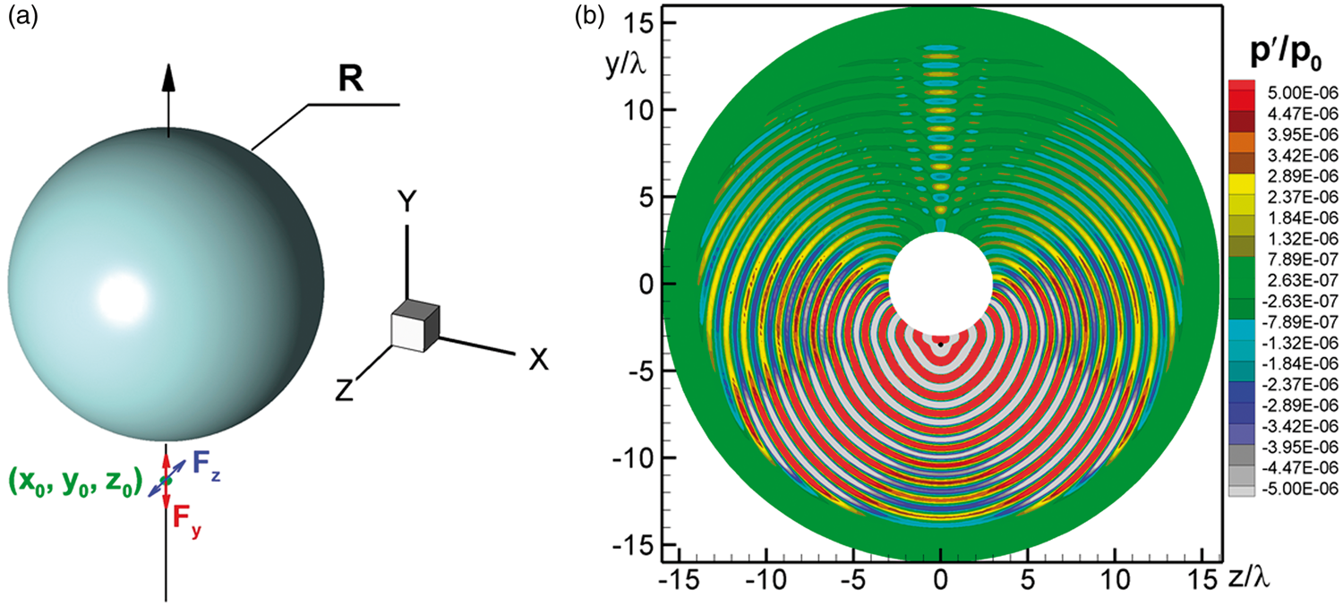
Dipole placed under sphere. (a) Geometry and (b) pressure field. Coordinates are normalized with the wavelength λ = R/3.
The “straightforward” identification approach we called PSFWH would calculate the solid-FWH sound field, and declare that “this is the sound of this part of the airplane.” Here, the sound field of the dipole is known analytically. The dipole is injected into the flow field via source terms
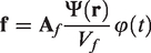
Here
Below we only show cases with a vertical dipole (Fy in the figure), but results with a horizontal dipole led to the same conclusions.
There is no flow, and the walls are treated as free-slip surfaces. The parameters are as follows: the wavelength is 1/3 times the sphere radius R, and the dipole is 1/2 a wavelength away from the surface. This creates interference patterns with approximately 45° for the dominant direction, as seen in Figure 1(b); other cases, with different offsets for the dipole, produced different patterns. As could be expected, the shielding by the sphere in the upward direction is very definite.
Results
We now turn to quantitative results, comparing the sound at a distance of 11 wavelengths λ from the origin, i.e. in the near-field, which allows comparisons with the direct output of the simulation, where the grid is still fine. The same conclusions would be reached for far-field sound, but the simulation cannot provide that, since the grid coarsens for large r and a sponge layer was introduced. In Figure 2(a) the simulation result, solid line, confirms the interference pattern and the shielding seen in Figure 1(b). The peak level at ±45° downwards is 30 dB higher than the lowest level, close to the straight-up direction. This result is accurately reproduced by the permeable FWH formula, independently of the radius of the FWH sphere (dotted and dash-dot curves). The sound field of the isolated dipole itself (long-dashed), in contrast, does not reproduce shielding; the only difference between the up and down direction is due to the difference in distance (14.5λ versus 7.5λ). It also misses the interference patterns. The sound field of the dipole with an opposite image dipole inside the sphere (not shown), which would be appropriate for a plane wall, does capture interference, to leading order, but it misses the upwards shielding and in any case does not provide a very practical method, with non-trivial geometries.
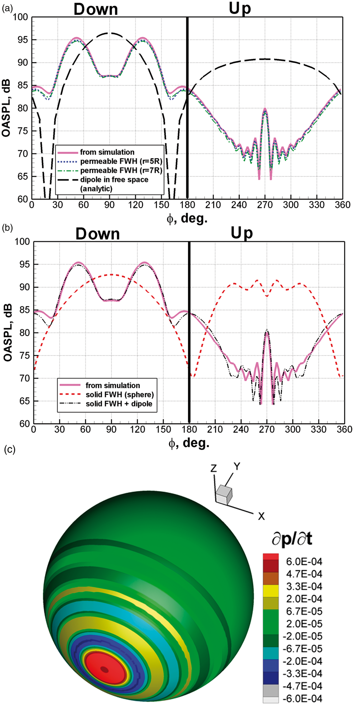
Sound extracted from simulation, and sound produced by integral formulas (a, b), and FWH surface term on the sphere (c). In frames (a, b), observers are located at
Of more interest are the results of the sphere’s solid-surface contribution, dashed curve in Figure 2(b), and its combination with the dipole, dash-dot-dot. In the upwards direction, the two almost cancel. This combination gives a very accurate answer, almost as good as the permeable formula. On a theoretical basis, this may be unsurprising, since this problem has no quadrupoles. However, in practice, this shows that while the dipole is the true source of sound, the calculation of the sound field must include the sphere’s contribution, which in aeronautical practice would mean the airplane’s fuselage and wing. Figure 2(c) shows the FWH integrand on the sphere, in other words the “footprint” of the dipole. Its extent appears to be a few times the distance from the dipole to the surface. This will be a guide in practice when designing FWH surfaces, solid or permeable, and even grids, that is here the upper hemisphere contributes very little.
Isolated bluff body over a range of Mach numbers
Problem statement and flow field
The body is a right parallelepiped, with unit height h, width 1.5h, and length 3h. The Reynolds number based on h is 105, and four Mach numbers from 0.0625 to 0.5 were considered. The flow is treated by DDES; the grid is seen in Figure 3 and has 340 by 245 by 245 cells in the (x, y, z) directions, and the time step is 5 × 10⁻³h/U. The grid is clustered at all the walls, with the near-wall step equal to 10−4h, which corresponds to not more than 1.5 in the law of wall units, except for the vicinity of the forward stagnation point. The lateral steps in the “wakes” of the refined grid near the walls are equal to 5 × 10⁻³h. Away from the wall, the wall-normal grid steps increase with the ratio of 1.3, until reaching Δ = 5 × 10⁻²h in all the three spatial directions, and then is kept constant up to the sides and the front face of the control FWH surface. The streamwise grid step at the closest end-cap is twice larger, 0.1h. At the highest considered Mach number M = 0.5, this grid ensures accurate resolution of the sound waves propagation inside the FWH surface up to Strouhal number based on the body height around 6.
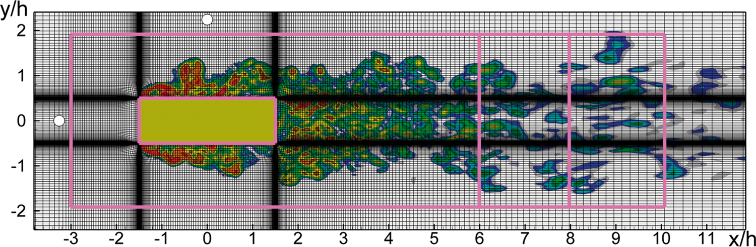
Fragment of grid, FWH surfaces, and vorticity contours.
The duration of the simulations was ≈80 time units, based on U and h, the last 40 of which were used for the FWH-based noise computations. Naturally, this leaves noticeable statistical noise in the spectra especially for Strouhal numbers of O(1), and scientific judgment is essential when interpreting the results. A decisive improvement in this respect would require orders of magnitude more computing effort. The figure also displays the FWH surfaces, vorticity contours, and the position of two near-field observers (white circles). The separation at the front corner naturally pours turbulence along the lateral faces and into the wake; the range of scales is rather wide. The usual gradual grid coarsening in the departure region is visible, and the eddy size adapts to the grid. Organized vortex shedding is not present due to the three-dimensionality of the shape.
Figure 4 displays the overall sound power level spectra, in raw form and then rescaled from different Mach numbers to M = 0.0625 using Curle’s M6 law. The power level is calculated relative to the reference power Wref = 10−12 W (PWL( f ) = 10log10(W( f )/Wref )), for the upward direction in the xy-plane (as if the acoustic pressure were independent of the azimuthal angle


Sound power level: (a) raw results, and (b) and (c) corrected using M6 scaling law. PWL: power level.
The spectra in Figure 4 reflect the broad-band turbulence. Curle’s theory is here quite successful, in two respects. First, the M6 law renders the Mach-number effect well, although the statistical noise on the spectra is too large for precise conclusions. Second, the solid-surface result is quite close to the permeable result, at least up to Mach 0.25 and more so at low frequencies, which is highly consistent with the key role of the product M×St. Still, the agreement appears to apply well outside the compact-body range, since M×St is well above 1. At M = 0.5, the permeable result is consistently higher, indicating a positive correlation between the dipole and quadrupole contributions. The apparent Mach-number power is between 6 and 7. Note that comparisons between FWH approaches in the same simulation are less hampered by statistical noise than comparisons between separate runs at different Mach numbers. We recognize that the “true” spectra would be significantly smoother, and judgment is needed for simulations of manageable cost when dealing with massive separation.
Figure 5 qualifies this finding about Curle’s theory, by examining results in specific observer directions rather than the sound power level. The far-field results at an angle of 90° repeat the findings of Figure 4, but those at 0° (directly upstream) do not: solid results are up to 10 dB lower than permeable ones. The latter results come from averaging the three end-caps, which we consider the most reliable approach. However, results from single surfaces were very close to the averaged results, suggesting that there is little contamination by end-cap effects. A factor that is more difficult to rule out is the effect of coarsening grid on the eddies, mentioned in the “Introduction” section, but this coarsening is most visible precisely between the three end-caps, so that it is reasonable to expect that it would force a difference between the results from the different end-caps. An end-cap at x = 4 would move outside the major coarsening region, but also begin to eliminate part of the focus region, and therefore well-resolved eddies and quadrupoles.
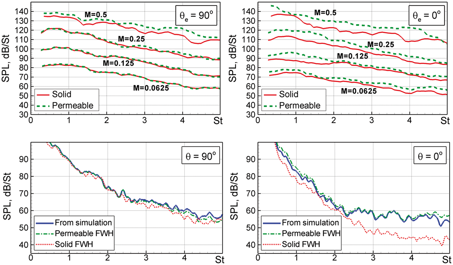
Spectra in different directions (
The lower frames of Figure 5 finally present direct comparisons between the two FWH predictions and the true sound of the simulation in the near field at M = 0.25; this is the “litmus test.” These show that the permeable-surface FWH formula reproduces the near-field sound in the simulation quite accurately for both considered near-field observers. Other than that, the near-field results are consistent with the far-field ones in the sense that at θ = 90° the solid and permeable FWH results are very close and at θ = 0° the noise from the solid surface is tangibly lower than from the permeable one. However, the difference between the solid and permeable predictions at θ = 0° in the near field is larger at the high frequencies, whereas in the far-field (top right frame in Figure 5) it is larger at the low frequencies. This reflects a significant input of high powers of 1/r in the near-field terms, which are absent in equation (1).
Overall, the results for a single bluff body producing massive separation and broad-band turbulence although free of a wide range of scales in the geometry tend to support Curle’s theory, even at Mach numbers which are not very small. There are however mild qualifications, particularly about the solid formula in the upstream direction. We now turn to more complex geometries.
Generic fuselage with a simplified landing-gear cavity
Problem statement and flow field
Next, a generic fuselage with a simplified landing-gear cavity is considered, as illustrated in Figure 6.
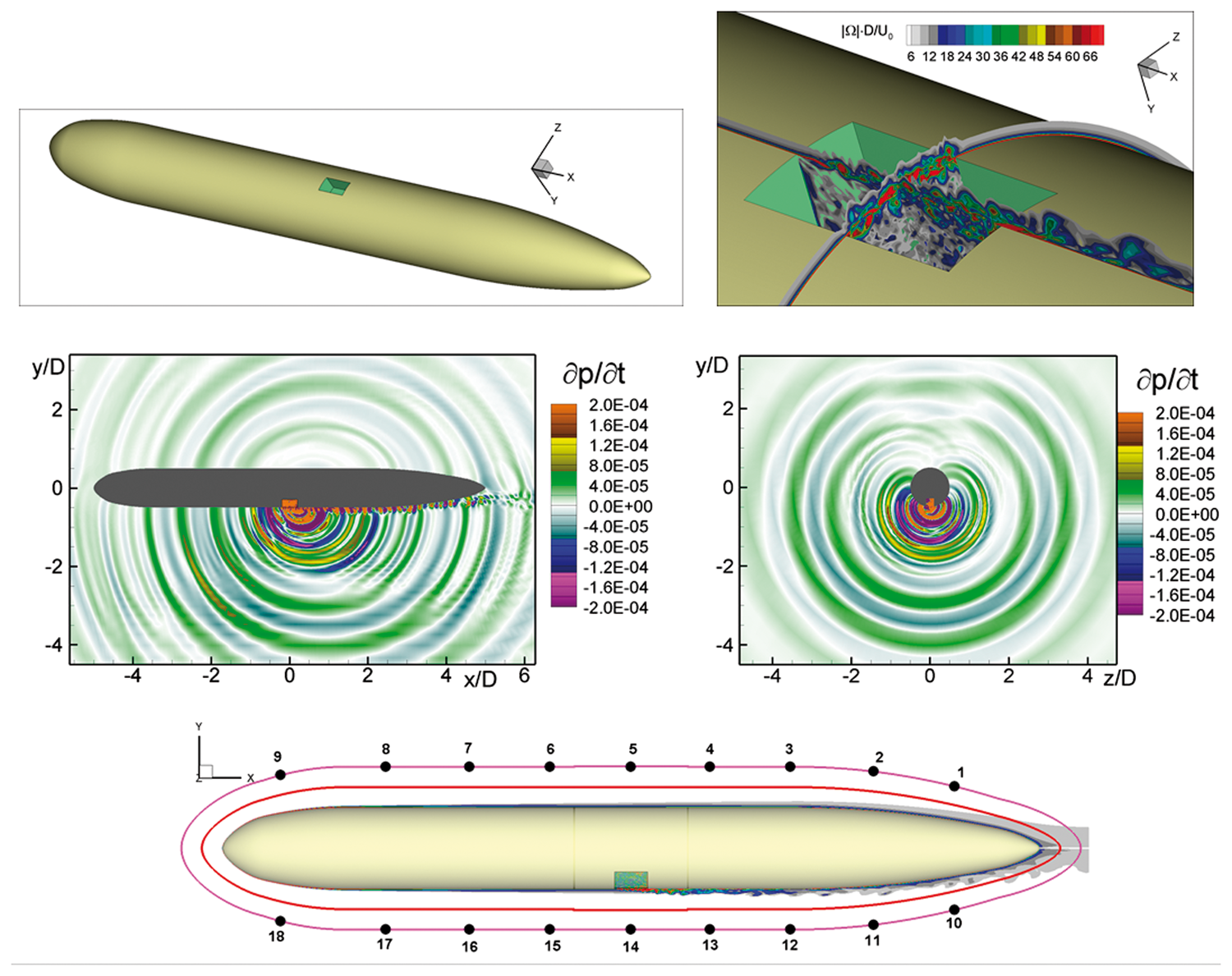
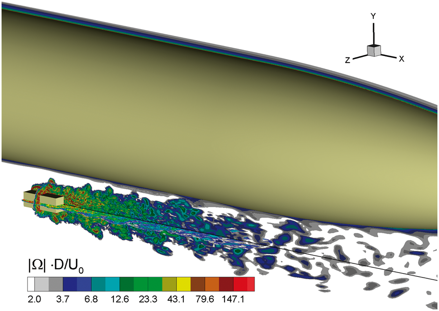
Simplified landing-gear cavity. Top left, geometry; top right, vorticity contours; middle, pressure field in XY and YZ planes (time derivative in the acoustic range normalized with
It has some key ingredients of the industrial problem, while being far less costly to compute, and separating cavity effects from bluff-body effects. This flow having quadrupoles, eddies crossing the permeable surface, and a departure region, the results will not be as close to perfection as in the first case, but we expect strong effects of shielding, with the PSFWH approach separating various parts of the surface in the FWH integral possibly leading to paradoxes.
The Mach number is 0.25 and the Reynolds number based on fuselage diameter D is 107. The cavity has length Lx = 0.4D, width Lz = 0.2D, and depth Ly = 0.2D. The flow is treated with DDES,
33
with most of the fuselage boundary layer in quasi-steady RANS mode. The grid used in the simulation (see Figure 7) has
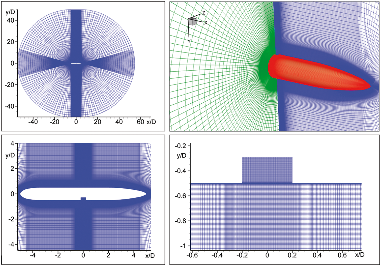
Some details of computational grid used for simplified landing-gear cavity flow.
Acoustic results
Figure 8 shows that unlike the solid-surface formula the permeable-surface FWH formula reproduces the near-field sound in the simulation very accurately, suggesting that the departure, end-cap, and similar effects are very moderate. This conclusion is however qualified when observing that the observer points are close to the permeable surface, so that the sound is primarily produced by local contributions to the integrals; this could conceal end-cap errors, for instance. The agreement would in a sense be “tautological.” Simulation results free of dissipation at larger distances are not expected with the grids we were able to run on. Vatsa et al. 13 to overcome this limitation extended a funnel-shaped fine-grid region all the way to the microphones, at a distance of the order of 2D, and the permeable results were only slightly more accurate. This was in the downward direction, like Point 14 is; it would be most valuable for them to repeat the exercise in the upward direction, emulating Point 5. The present comparison, at least, strongly suggests that the FWH utility is free of errors. Appelbaum et al. 20 conducted a very similar test, already reporting the same success only for the permeable surface. Far-field permeable predictions are therefore also considered reliable. This includes the strong sheltering, since the sound level at Point 5, above the body, is about 25 dB lower than at Point 14, below it; this is very consistent with Figure 6. This result, observed at a distance of D/2 from the fuselage, may not apply for large distances. The peak is at a Strouhal number close to 3.5; compare with the rough visual estimate of 4. On the other hand, the spectrum shape for low frequencies up to St ∼ 5 is similar although by no means identical at those two points, which we have not explained yet. The plateau over St=(8, 15) for Point 14 is also difficult to predict.
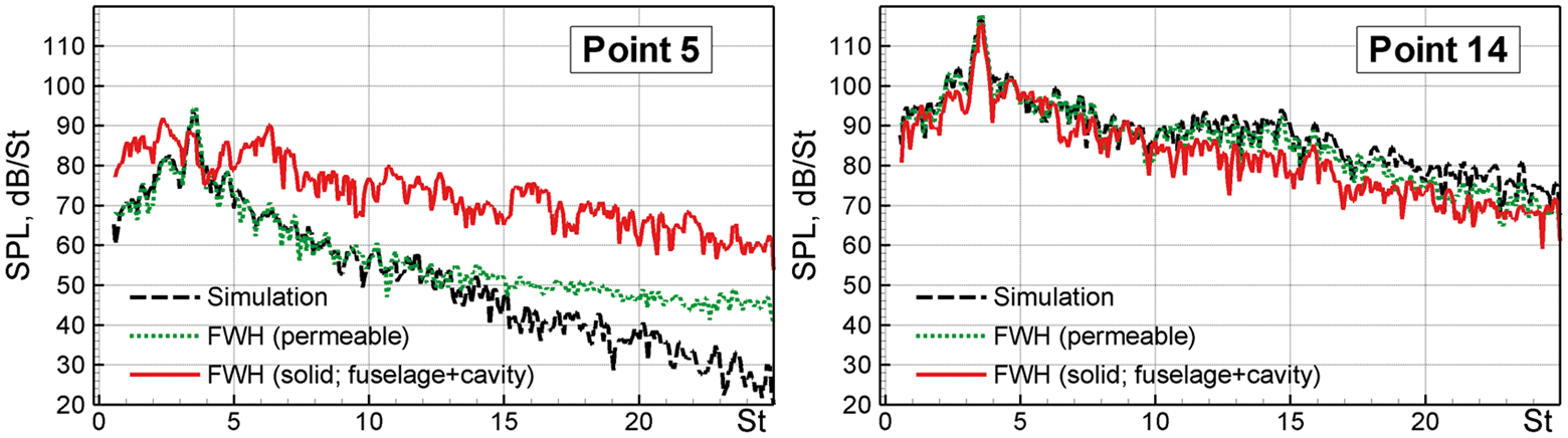
Spectra from simulation and from solid- and permeable-surface integrals at two points above and below fuselage (see Figure 6). FWH: Ffowcs Williams–Hawkings; SPL: sound pressure level.
Figure 9 presents another test of the near-field permeable utility of Abalakin et al. 35 In theory, the FWH formula returns zero for the pressure field inside the surface. This can be viewed as a “compatibility condition” for the distribution of all the terms on Σ in equation (1). The figure shows that the level drops by at least 26 dB when crossing the surface inwards, which is quite satisfactory and strongly suggests that the quadrupoles external to the permeable surface have a very small impact. It also suggests that the simulated flow field is free of strong “viscous-like” effects outside the surface, which were discussed in the “Introduction” section, and that the grid is fine enough near the surface for an accurate integration. The fact that the integrand contains wavenumbers twice as large as the flow field does presents a challenge to accurate numerical integration (this phenomenon depends on the exact formulation, and in equation (1) it is essentially driven by steep variations of the retarded time, for high frequencies).
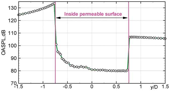
Distribution of near-field overall sound-pressure level along vertical axis (x = z = 0), as produced by permeable FWH integration. OASPL: overall sound pressure level.
Figure 10 presents far-field results of different approaches, which are not as simple as for the sphere-dipole case. Namely, it compares sound power spectra in the upwards and downwards direction computed with the use of solid FWH and permeable FWH approaches, the latter with two nested surfaces which give virtually identical spectra. The figure shows that according to permeable FWH the difference between directions is weaker than in Figure 8, around 10 dB in terms of the peak values, due to this applying in the far-field. However, this is still a large difference.
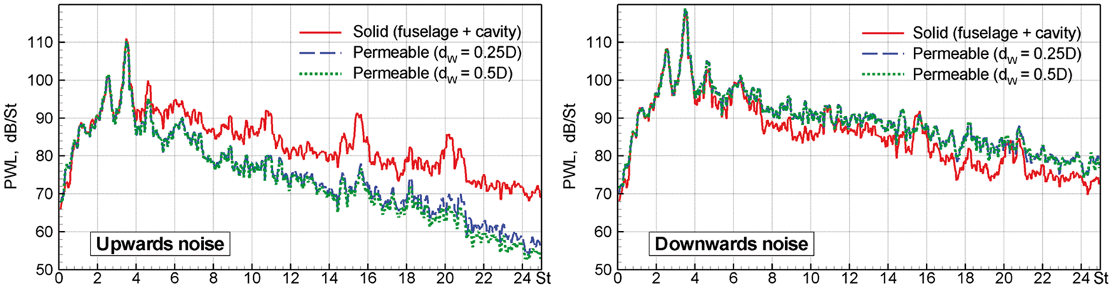
Sound power levels in the vertical direction with different FWH approaches. Far-field results. Left: upwards; right: downwards. PWL: power level.
Other than that, the solid and permeable results in Figure 10 are almost identical up to a Strouhal number of 4, and in particular the peak at St ∼ 3.5 is identical. For St larger than 4, the two results diverge, and the solid-FWH calculations essentially miss the shielding effect, even though these are results with the full surface (both cavity walls and fuselage skin), an approach which was successful for the sphere-dipole case. This appears to reflect the quadrupole contribution, which would have constructive interference with the surface terms in one direction, and destructive interference in the other direction. The relative success of the solid formula for low frequencies (which would not be relevant in airline practice) followed by an abrupt divergence has not been explained yet; in particular, a simple argument such as the source being compact does not seem to apply since λ ∼ D. This is if the entire fuselage is viewed as the source, as opposed to the cavity, of depth D/5, not to mention the eddies in the shear layer, of smaller size yet.
Figure 11 gives a more detailed idea on the relationship between the sound levels predicted with the use of different approaches including the PSFWH with partial surfaces being the fuselage skin w/o the cavity and the cavity walls only. Strouhal numbers below 4, which are too tainted by statistical imperfections, were not included. In addition to the considerable difference between the solid and permeable results mentioned above, the figure strongly confirms our conjecture in the “Partial surface integrations” section about the apparent contribution of the cavity walls: it has almost no directivity in the transverse vertical plane, while its directivity in the longitudinal plane is almost the same upwards and downwards, but curiously includes a much higher level in the upstream direction. The directivity for the ceiling alone (not shown) exactly confirmed our conjecture in the “Partial surface integrations” section. The directivity of the permeable result, peaking at 50° downwards, is fully consistent with Figure 6.
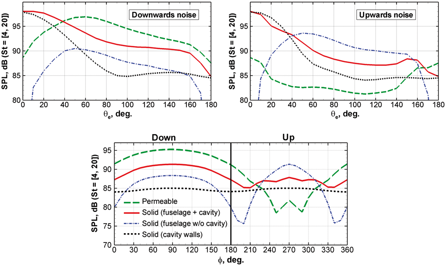
Far-field sound pressure level directivity curves for two symmetry planes of the configuration reduced to emission distance 1.0D. The SPL is computed by integration of spectra over the Strouhal number range St = [4, 20]. Upper graphs: XY-plane; lower graph: YZ-plane. SPL: sound pressure level.
The dominant frequency is of interest. If we assume that the large eddies in the mixing layer propagate at half the freestream velocity, St = 3.5 corresponds to an eddy spacing of D/7, which is much larger than the visual spacing in the simulation, based on Figure 6. The Strouhal number based on cavity length L is 1.4, which would approximately correspond with the third Rossiter mode (using StL = (n −γ )/(M + 1/κ) with γ = 0.25 and κ = 0.57). Finally, the cavity length and depth are 0.4D and 0.2D, respectively, so that conjectures based on half- or quarter-wavelength modes are not satisfied either. In other words, various plausible estimates based on the geometry or the flow visualization fail to predict the observed frequency.
Overall, our results for the generic fuselage with a simplified landing-gear cavity configuration strongly support the permeable-surface FWH formula, and indicate that the solid-surface formula can be highly misleading regarding the actual sources of sound, and in particular fail to capture directional effects. This conclusion applies only for frequencies above the primary peak, but in a typical airliner, St = 3.5 would be below 50 Hz, and therefore of little interest; St ∼ 50 is far more relevant in flight.
Generic fuselage with a simple bluff body
The next problem aims at turbulence generated by massive separation in the vicinity of a large body. The shape is again simple, a right parallelepiped of thickness h, length 3h, and width 1.5h with h = 0.1D, free of disparate scales (unlike real landing gear), and with sharp corners which minimize the effects of Reynolds number and turbulence model. The turbulence will originate away from the fuselage, but still interact with it. The flow Mach number and the Reynolds number based on D are the same as in the fuselage-cavity problem considered in the previous section.
Figure 12 shows the geometry and the grid used in the bluff body block with size

Geometry of the fuselage with bluff body configuration and grid in the bluff body block.
Instantaneous vorticity contours.
Figure 14 shows that the pressure perturbations generated by the bluff body interact intimately with the fuselage, even though the turbulence itself almost does not make contact with the fuselage surface (based on the vorticity contours in Figure 13). The figure also makes the shielding in the upwards direction again very visible. This flow has a much wider range of wavelengths than the previous one; the waves which reach above the fuselage have a wavelength close to 0.6D. The damping by grid coarsening appears definite around 3D below the fuselage, but is not relevant to the permeable surfaces.

Time-derivative of the pressure in the acoustic range.
The far-field spectra in Figure 15 reveal much about all approaches. First, similar to the fuselage-cavity configuration, the permeable approach captures the shielding, which is of the order of 8 dB, but the solid approaches essentially fail to. Second, the solid predictions are unnatural for the upwards direction. Namely, the contribution of the fuselage in this direction is about 5 dB larger than that of the bluff body although physically, the latter is a major sound source. Overall, considering this and, also, based on the results obtained with the use of the permeable FWH surface, the PSFWH answers are quite different and misleading.

Sound power levels in upwards direction (left column) and downwards direction (right column). PWL: power level.
Note finally, that the simulation results presented above were repeated on a grid with the fuselage block refined by a factor of 2 in the azimuthal and polar directions (this Grid 2 had around 62 million cells). This improved both the resolution of the simulation and of the FWH integration. This however did not lead to any systematic alteration of the noise predictions discussed above. See Figure 16 comparing the SPL spectra obtained on the two grids at θe = 90° for the upwards and downwards direction with the use of both solid and permeable FWH surfaces. The differences in Figure 16(a) for St < 6 are noted, but may be statistical. This supports the accuracy of the computations, at least, in terms of the sound waves’ propagation and their scattering by the fuselage surface.

Effect of grid on the far-field SPL spectra at
Finally, Figure 17 addresses the impact of the cross-term between dipoles and quadrupoles, discussed in the “Introduction” section (JSV13-16). The quadrupole term
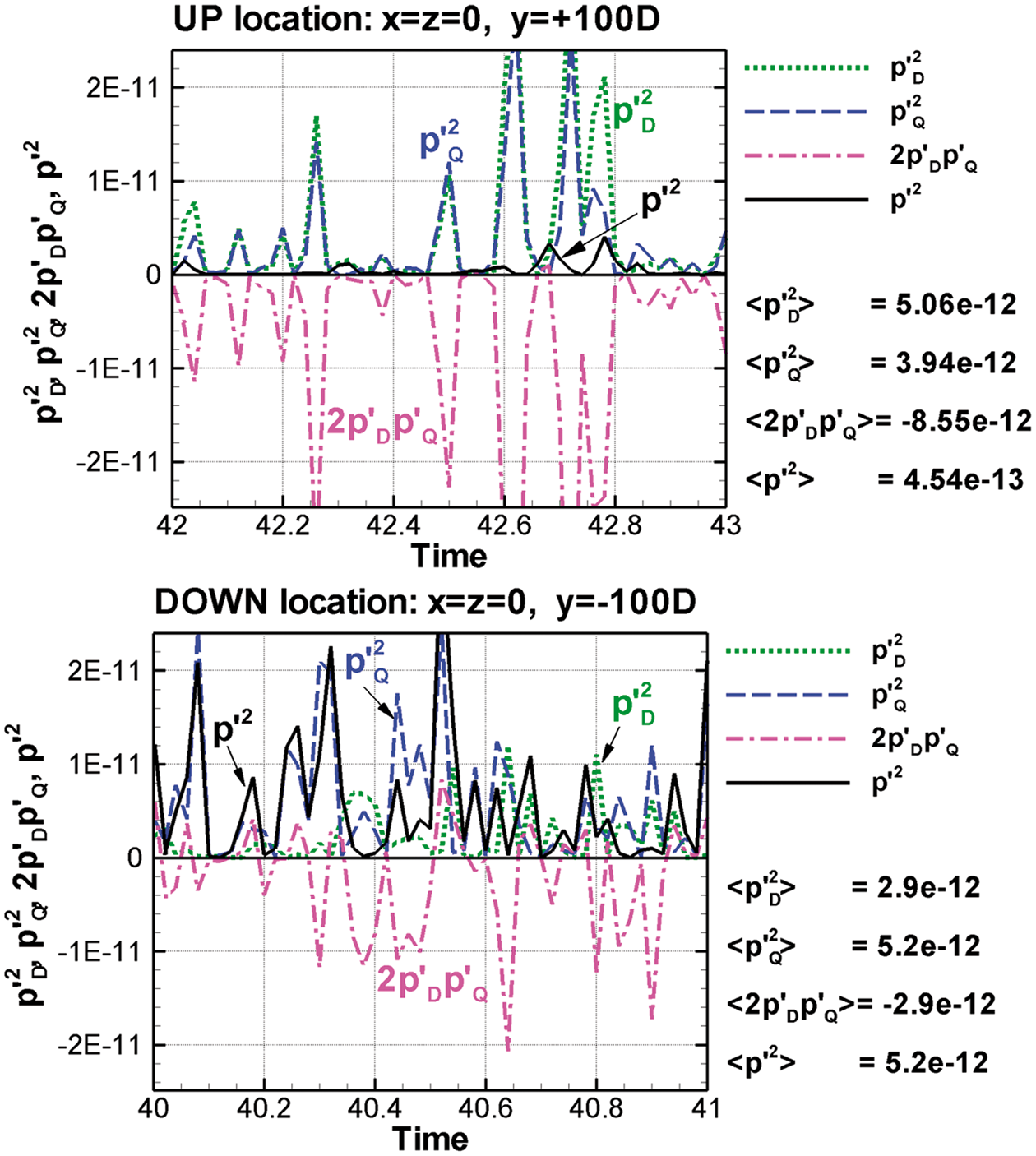
Time-domain traces of the dipole, quadrupole, and cross-term contributions to the square of pressure,
Conclusions
We presented simulations and acoustic results via different versions of the FWH integral formula for a set of four model problems relevant to airframe noise, including in some cases wide variations of the Mach number, and moderate variations of the grid spacing. Curle’s widespread low-Mach-number theory is emphasized in two respects: his prediction that the solid-surface terms dominate, and that aerodynamic sound scales like M6 (for
Few of our questions had simple answers, and the success of Curle’s theory is case-dependent. This paper adds knowledge to the JSV13 line of thinking, without exhausting the subject. Sharp answers are made more difficult by the statistical noise in the spectra; presuming that this effect scales with
Conclusive results for the near-field sound showed that the permeable-surface FWH formula gives results that are as accurate as those of the simulation. The design of that surface is based on flow visualization and “common sense,” but careful grid generation with very gradual stretching is needed. By extension, the same formula gives far-field results that are as accurate as the simulation is, whereas the solid-surface formula fails often, especially when shielding effects are powerful. In addition, the partial surface FWH approach is close to illusory.
Progress in both research and industrial computational aero-acoustics will depend on the present results being accepted by the community, and confirmed in different enough flow solvers, FWH utilities, and without excessive sensitivity to the placement of the permeable surface. This will take time. The scientific community very much values independent findings, and for good reason. A favorable development would be the selection of one of the present test cases for a future workshop, in the BANC or other series. The range of scales in the geometries was not very wide, and it must be remembered that pantographs, on trains, and brake lines, on airplanes, are very thin and generate high frequencies. This will severely challenge the creation of grids that are fine enough to resolve such phenomena over a large-enough volume to reach a global permeable FWH surface. The accurate simulation of landing gear, 5 m tall and with 1 cm tubes shedding vortices (well within the audible range), is clearly demanding of many billions of grid points and tens of thousands of time steps; this is even before attempting to calculate the radiated sound. The “brute force approach” is not practical yet, recent claims at conferences notwithstanding.
Footnotes
Acknowledgements
The calculations were performed at the Computer Center “Polytechnichesky” of St Petersburg Polytechnic University. We enjoyed excellent discussions with Dr U. Michel, Prof. S. Lele, Dr T. Ricciardi, and Dr W. Wolf. Finally, we thank Drs A. Duben and T. Kozubskaya for sharing their near-field FWH utility.
Declaration of conflicting interests
The author(s) declared no potential conflicts of interest with respect to the research, authorship, and/or publication of this article.
Funding
The author(s) received no financial support for the research, authorship, and/or publication of this article.