Cost-effective hybrid RANS-LES type method for jet turbulence and noise prediction

Abstract

Jets at higher Reynolds numbers have a high concentration of energy in small scales in the nozzle vicinity. This is challenging for large-eddy simulation, potentially placing severe demands on grid density. To circumvent this, we propose a novel procedure based on well-known Reynolds number (Re) independent of jets. We reduce the jet Re while rescaling the boundary layer properties to maintain incoming boundary layer thickness consistent with high Re jet. The simulations are carried out using hybrid large-eddy simulation type of approach which is incorporated by using near-wall turbulence model with modified properties. No subgrid scale model is used in these simulations. Hence, they effectively become numerical large-eddy simulation with Reynolds-averaged Navier–Stokes covering the full boundary layer region. The noise post-processing is carried out using the Ffowcs-Williams-Hawking approach. The simulations are made for Mach numbers (M) of 0.75 and 0.875 (cold and hot). The results for the overall sound pressure level are observed to be within 2–3% of the measurements, and directivity of sound is also captured accurately for both the cases. Hence, the low Re simulations can be more beneficial in saving time and cost while providing reasonably accurate results.

Keywords

LES Jet Noise Hybrid RANS-LES Ffowcs Williams-Hawking method

Introduction

Aircraft noise is a critical issue for people living in the vicinity of airports and has adverse effects on healthy living. Jet noise is the second largest contributor in total engine noise after fan noise. One of the three new targets of Advisory Council of Aeronautical Research in Europe, to be achieved for clean engine by 2020, is noise reduction by 10 dB.¹ Therefore, it is a critical issue for engine manufacturers to be able to predict noise levels using economical methods that allow testing of noise reduction techniques. Various research groups are focused on addressing this issue. Some are inclined on doing what is called in DeBonis,² the rigorous large-eddy simulation (LES). This is good for development of methods and understanding flow physics at a deep level. This paper on the other hand focuses on practical LES. It involves validating LES for industrial flows in realistic configurations. The goal is to come up with a robust technique which is economical and can be used confidently by the industries without having to think about different dependency factors while gaining reasonably accurate solutions. The hybrid RANS–NLES technique has been used in past by Eastwood and Tucker.³ Through the use of a RANS layer, it has been shown to reduce the high-density grid requirements near surfaces, eliminating non-physical separation from convex nozzle surfaces. The NLES component reduces excessive dissipation when using robust industrial solvers through subgrid scale model omission. Most studies into jet noise tend to be at lower Re.^4–6 As we move towards more engine realistic jets, the Re increases. A few researchers have tried running jets at higher Re^7,8 but have not successfully validated their approach. Noise levels are clearly over-predicted in Fayard et al.⁸ Although Andersson et al.⁹ report data comparison for a case run on lower Re than that of experiments, they do not mention anything about the boundary layer state at nozzle exit. Jets are Re independent beyond the boundary layer region above a threshold value of order 10⁵.^10,11 However, with increasing Re, more energy will be contained in small scales. This will impact LES solution in following ways:

For a fixed filter, the numerics will become more stressed due to more energy interacting at the filter scale;

The LES subgrid scale model will need to model a greater fraction of turbulent energy.

Since, for a jet, the size of large scales increases downstream for a fixed filter width, moving downstream the characterization of energy in the smaller scales becomes less of an issue. For example, DNS of a jet reports that the ratio of the energy in the small to large scales is 42%, 12% and 5% for $x / δ ω o$ = 40, 60 and 80, respectively, where $δ ω o$ is the initial vorticity thickness in Bodony and Lele.¹² If the LES modelling sits in the inertial range, as it should, then the turbulence energy spectrum can be expressed as, following Bodony and Lele¹²

E (k) ~ \frac{ε 2 / 3}{k 5 / 3}

(1)

where k is the wave number. Then it follows that the energy under the filter E_under is given by

E under = \int_{k c}^{\infty} E (k) d k ~ \frac{ε 2 / 3}{k_{c}^{2 / 3}},

(2)

where k_c is the cut-off wave number of the subgrid filter. Now, we know that the dissipation

ε \approx u' 3 / l

where

u'

represents the turbulence fluctuation levels and l is the length scale. The l will increase linearly with downstream distance while

u'

will remain relatively constant. Hence,

E under \propto x - 1

and the energy contained with the scales will decrease with downstream distance x. The foregoing scaling argument from Bodony and Lele¹² implies that the greatest area of numerical and LES model sensitivity will be near the jet outlet at high Reynolds numbers. The issue of grid dependency thus arises for high Re LES. Hence, here the idea is to capture the larger scales and the basic structure of the turbulence by running the simulation at lower Re while preserving the momentum thickness Re in the upstream boundary layer (as in high Re rig condition). Figure 1 shows a schematic of the regions in the jet and the corresponding treatment applied to them.

Figure 1.

Re-sensitivity zones in various regions of jet flow.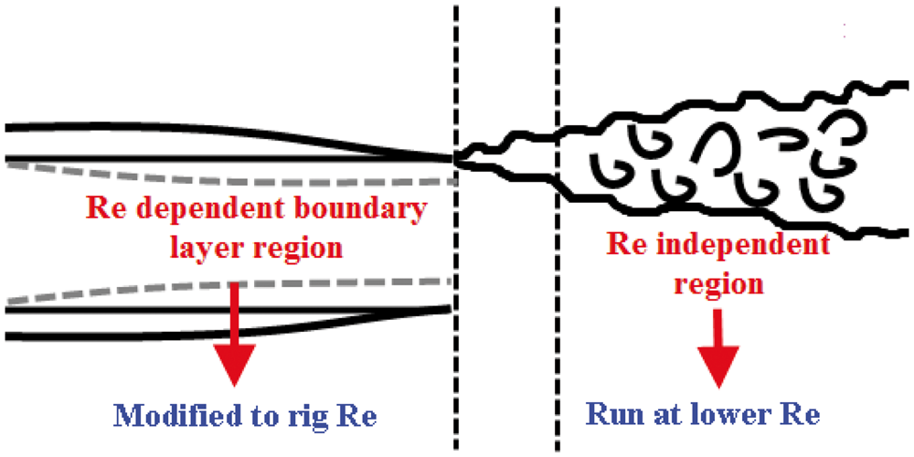

This paper is set out as follows. First the numerical methods are discussed. The case setups are given. The application of the approach is then demonstrated for cold jets at two Mach numbers. Also, some hot jet results are presented.

Computational method

Main computation

The solver is second order accurate in space and time. Although sophisticated higher order schemes will be more accurate, second order-centered schemes are known to give sufficiently accurate results. There is also the relative ease of implementing them in a CFD code to be considered. The solver used is node-centered control volume based. The second order central difference for flux calculation is represented by the equation below

Φ f = \frac{1}{2} (Φ L + Φ R) - \frac{1}{2} | A | [φ L - φ R]

(3)

The second term is a smoothing term. This can be approximated as

\frac{1}{2} | A | [φ L - φ R] = \frac{1}{2} ɛ | A | [{\tilde{\nabla}}_{L}^{2} φ - {\tilde{\nabla}}_{R}^{2} φ]

(4)

with tunable smoothing parameter ɛ and Jacobian matrix A. This is distributed in the domain as shown in Figure 3. The smoothing parameter is increased towards boundaries. This yields a sponge zone which helps in avoiding reflection of spurious waves from boundary. The lowest value used in these simulations is 0.3. This value is tuned to get a minimum for which stable solution can be obtained. The code has been extensively tested for canonical problems for its accuracy¹³ and has been successfully used to predict both the flow and acoustic fields for several single stream¹⁴ and coaxial jets.¹⁵

Figure 2.

Blending between RANS and NLES zone through wall distance function.

Figure 3.

Smoothing control parameter(ɛ) distribution in domain.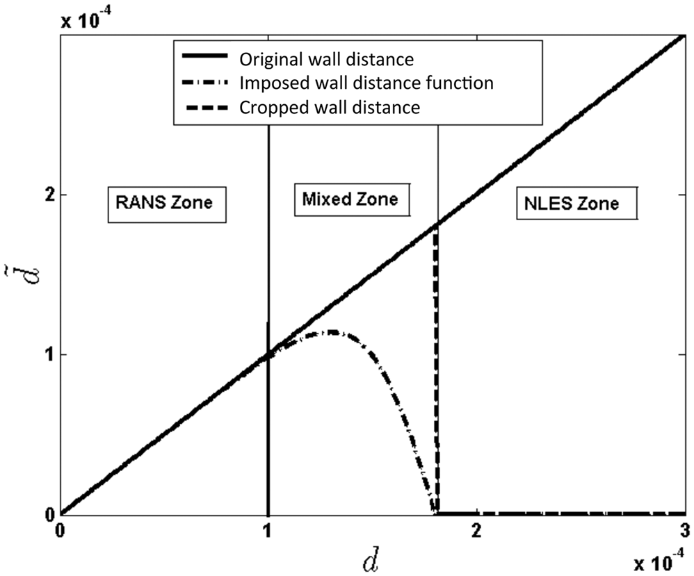

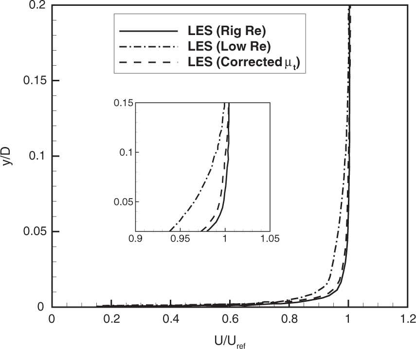
The boundary layer region uses the Spalart Allmaras (SA) RANS model. The eddy viscosity μ_t yielded from this is scaled down to keep Re consistent with actual jet conditions in the boundary layer region. Figure 9 shows a boundary layer velocity profile comparison. This is explained later in Results and discussion section. However, the key point is that the expected rig scale velocity profile is matched in the lower Re LES. >

The hybrid RANS–NLES scheme is incorporated by simply modifying the wall distance using Hamilton-Jacobi (HJ) equation.¹⁶ This gives smooth blending between the RANS and NLES regions. The HJ equation is given below

| \nabla \tilde{d} | = 1 + f (\tilde{d}) \nabla 2 \tilde{d} + g (\tilde{d})

(5)

where

f (\tilde{d}) = ɛ o \tilde{d} and g (\tilde{d}) = ɛ 1 (\frac{\tilde{d}}{d c}) 2

(6)

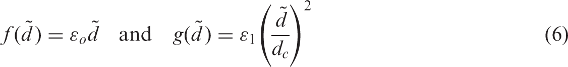
The function f( $\tilde{d}$ ) controls the smoothing between the exact wall distance, d, zone needed near walls for the RANS model and the d = 0 NLES zone with its zero explicit implied modelled LES content. The g( $\tilde{d}$ ) function gives biasing $d c = δ$ , the boundary layer thickness. The parameters $ɛ o$ and $ɛ 1$ are constants. The form of the $\tilde{d}$ distribution is shown in Figure 2. The full line in Figure 2 shows the raw wall distance as used by a typical RANS model. The dashed line shows a cropped wall distance. This is then smoothed to the chain-dashed line as shown in the figure.

The RANS layer thickness is such that it covers the boundary layer region. Note that the RANS layer is ultimately used in a frozen state. This saves wasted computational effort, solving an additional transport equation through a lengthy LES run.

Acoustic post-processing

The Ffowcs Williams-Hawkings (FW-H) approach is used to evaluate farfield noise. The acoustic post-processing is done on instantaneous flow data stored at points on a surface enclosing the noise sources (but outside them). In jets, the main sources of noise lie in the shear layer. Hence, we need to enclose the region of fluctuating quantities inside our surface. The relation for acoustic pressure, $p' = p (x, t) - p o$ is

4 π | x | p' (x, t) = \frac{x i x j}{| x | 2 c 2} \frac{\partial 2}{\partial t 2} [\int V T ij dV] + \frac{x j}{| x | c} \frac{\partial}{\partial t} [\int S p' n j + ρ u j u n dS] + \frac{\partial}{\partial t} [\int S ρ u n dS]

(7)

where S is the FW-H surface and V is the volume outside S. Figure 5 shows the FW-H surface location with respect to the flow and domain. The vector x defines the observer position. The integrals in the square brackets are calculated at a time when sound was generated. This is at

τ r = t - \frac{| x - y |}{c}

where y is the source location. Projections of the vector of outer normal to S are n_j. Note,

T ij = ρ u i u j + p ij - c 2 ρ' δ ij

is the Lighthill tensor. In this

ρ' = ρ - ρ o

is the acoustic density,

p ij = p δ ij - τ ij

the total stress tensor. Also, τ_ij is the viscous stress tensor which can be neglected for high Re flows. The final Lighthill tensor is

T ij = ρ u i u j + (p' - c_{o}^{2} ρ') δ ij

where u_j and u_n are the velocity and normal velocity components, respectively. The farfield sound can be calculated in terms of overall sound pressure level (OASPL). This is computed using the pressure history given by FW-H solver at particular observer location

OASPL = 20 \log 10 (\frac{p' rms}{2 \times 10 - 5})

(8)

Case setup

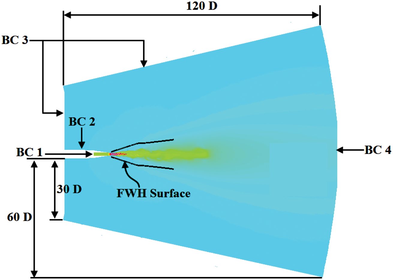
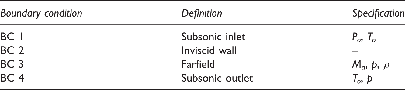
A round converging nozzle is used for all simulations. Figure 4 shows images of the geometry. The nozzle diameter, D, is 0.106 m. Figure 5 shows the overall domain size and labels the boundaries used. Table 1 summarizes various boundary conditions. The domain has radial extent of 60D and axial length of 120D. The domain is designed to make it suitable for noise calculation so as to avoid any reflection from the boundaries.

Figure 4.

Geometry of nozzle.

Figure 5.

Domain, dimension, boundary conditions and position of FW-H surface.

Table 1.

Boundary conditions for Figure 5.

Boundary condition	Definition	Specification
BC 1	Subsonic inlet	P_o, T_o
BC 2	Inviscid wall	–
BC 3	Farfield	M_a, p, ρ
BC 4	Subsonic outlet	T_o, p

Structured hexahedral meshes are the most suitable for LES.¹⁷ A key grid requirement is to resolve the jet shear layer and capture the initial turbulent structures. The strategy used for meshing is thus an O-mesh around the H-mesh block at the jet centreline. Figure 6 shows mesh cut planes at the jet exit. Moving from left to right, the images represent views zoomed in closer to the jet axis. The high shear layer resolution at the nozzle’s the edge is evident. Figure 7 shows the three-dimensional views of the mesh topology again showing the mesh following shear azimuthally as well as axially. Grid densities of 18 and 50 million cell meshes are generated. The 18 million cell mesh has 120 azimuthal nodes with $Δ x$ = 0.005D and $Δ r$ = 0.000045D across the shear layer to capture the initial instability in nozzle lip region. The 50 million cell mesh on the other hand contains 180 azimuthal nodes with $Δ x$ = 0.003D and $Δ r$ = 0.000025D across the shear layer. This results in around 40 and 70 nodes across the shear layer in 18 and 50 million cell meshes, respectively.

Figure 6.

YZ-plane mesh at jet exit.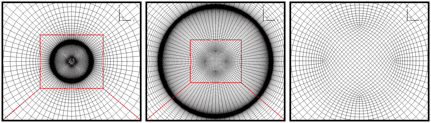

Figure 7.

3D mesh.

Five LES simulations were run at different grid densities. Table 2 gives the conditions at which the cases were run with their corresponding Re. Case 1 and Case 2 were run at a lower Re(=10⁵) by reducing the nozzle diameter by a factor of 10. However, the relative boundary layer thickness was fixed to represent the rig Re. This was achieved by uniformly reducing μ_t by a factor of 10 in SA RANS model uniformly covering boundary layer. These cases were run for 18 and 50 million cell meshes at both the rig and LES Re. Case 3 for a hot jet was run on the rig Re. The high temperature lowers the jet Re automatically. This eliminates the need for using the Re lowering technique. A typical 18 m cell simulation takes 400 h using 1024 cores (approximately a month). On the other hand, a 50 m simulation takes approximately thrice the resources used for 18 m simulation. The non-dimensional time,

t *

is defined as the time taken by the flow to travel a distance equal to one diameter and is defined as

t * = \frac{tU j}{D}

. The averaging for Case 1 and Case 3 is done up to 80

t *

and for Case 2 up to 140

t *

. The variables are further averaged azimuthally.

Table 2.

Test conditions.

Jet conditions	Case 1	Case 2	Case 3
Jet velocity (m/s)	255	300	300
Jet Mach No. (M_j)	0.75	0.875	0.56
Acoustic Mach no. ( $M \infty$ )	0.75	0.875	0.875
Jet temperature (K)	325	330	760
Rig Reynolds no.	1.15 × 10⁶	1.2 × 10⁶	4.0 × 10⁵
LES Reynolds no.	1.15 × 10⁵	1.2 × 10⁵	4.0 × 10⁵

To capture the directivity of noise, the OASPL and the FW-H surface used can be expressed using the equations below

r = {2.75 \frac{x}{10} + 1.25 0 \leq x / D \leq 10 \frac{x - 10}{20} + 4 10 < x / D < 30

(9)

Note that no closing disk is used. A full exploration on optimal surface locations can be found in Naqavi et al.¹⁴

The points at which the OASPL is calculated can be seen in Figure 8. Each observer location is placed along an arc with the center at the jet exit plane. The arc radius is equal to 120D and data on the arc is stored at 10° increments from centerline.

Figure 8.

Location of points where OASPL is calculated with respect to the jet exit.

Figure 9.

Boundary layer profiles demonstrating correction effect.

Results and discussion

The higher rig Re boundary layer properties are conserved while running the simulation at low Re. The boundary layer profiles are shown in Figure 9. The solid black line represents rig Re boundary layer state at the nozzle exit. The dot-dashed black line shows the LES at the lower Re. The dashed black line shows the boundary layer adjusted to match that in the rig through scaling μ_t.

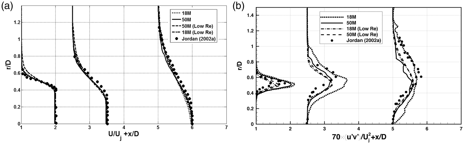
Figures 10 and 11 compare the simulations with measurements in Andersson et al.¹⁸ (Note: The measurements reported are from Jordan 2002a – Internal project report) and Bridges and Wernet.¹⁹ Figure 10(a) shows the centerline (U) velocity and Figure 10(b) stream wise fluctuating ( $u' rms$ ) velocity distributions. Figure 11 shows the radial profile comparisons for velocity and primary Reynolds shear stress. The dotted and dot-dashed lines represent 18 m and solid and dashed lines the 50 m mesh simulations. The solid and dotted lines in Figure 10 show simulations at rig Re. These lines show grid sensitivity. The lower Re (with corrected μ_t in the boundary layer) shown by the dashed and dot-dashed lines do not show much mesh sensitivity and follow the experimental data represented by the symbols. The measured centerline $u' rms$ distribution of Andersson et al.¹⁸ erroneously shows high turbulence levels inside the nozzle. This must arise from some facility issue. Such high levels are not evident in the measurements of Bridges and Wernet.¹⁹ Hence, we can see from the data of Andersson et al.¹⁸ a higher peak turbulence level at the end of potential core than suggested by the LES. The radial profiles are shown at $x / D = 1.0, 2.5$ and 5.0. Simulations are able to capture peak turbulence levels. Hence, as will be shown later, they also show encouraging noise data agreement.

Figure 10.

Centerline average velocity distributions for different mesh densities – case 2. (a) Mean velocity and (b) streamwise fluctuating velocity.

Figure 11.

Radial profiles for different mesh densities – Case 2. (a) Mean axial velocity and (b) Reynolds shear stress.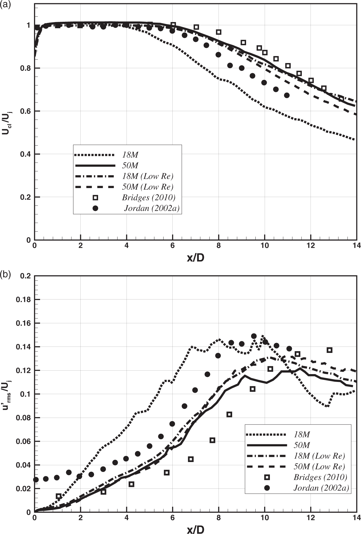

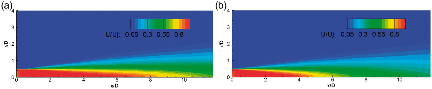
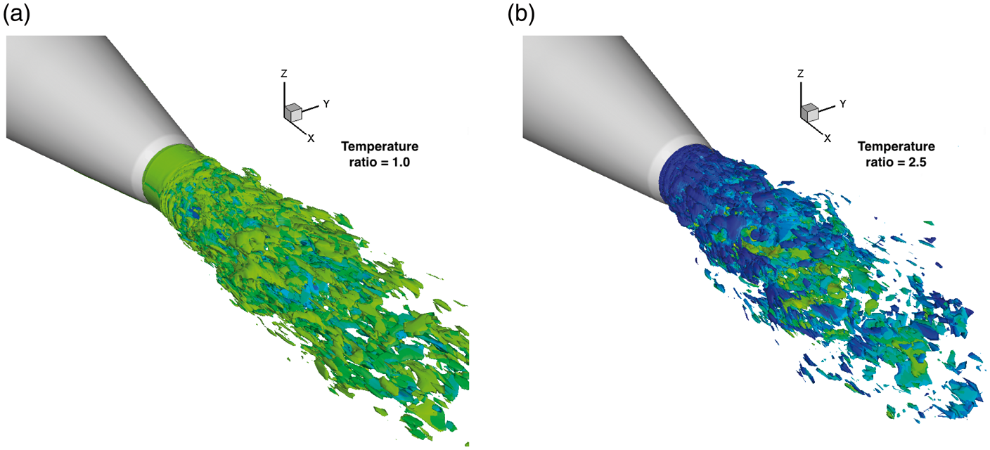
Instantaneous and time average flow pictures are show in Figures 12 and 13, respectively. The frames are non-dimensionalized axis with respect to jet diameter, D. Figure 12 contrasts instantaneous velocity contours for cases 2 and 3. Both frames compare the jet development for different temperature ratios. Figure 13 shows the averaged contours for both the cases. As would be expected, the potential core for hot jet is much shorter than the cold jet. This demonstrates fast mixing of a lower density hot jet with the ambient air. Vorticity iso-surfaces for the cases are shown in Figure 14. The iso-surfaces are flooded with temperature. This gives an idea about the temperature ratio of the jet to ambient air.

Figure 12.

Instantaneous velocity contours: (a) case 2 and (b) case 3.

Figure 13.

Average velocity contours: (a) case 2 and (b) case 3.

Figure 14.

3D Vorticity iso-surfaces flooded by temperature: (a) case 2 and (b) case 3.

OASPL at various observer locations as described in Figure 8 were calculated and the results are compared with measurements of Andersson et al.¹⁸ (Note: The measurements reported are from Jordan 2002b – Internal project report.) and Tanna²⁰ (for M = 0.875). The noise data are scaled to 100D in Figure 15(a) to (c). The results show encouraging agreement being within 2–3% of the experimental data. However, as shown in Shur et al.,²¹ the results can be sensitive to the FW-H surface location. Figure 15(d) shows that the current process can capture the influence of Mach number and temperature. This combines current results for M = 0.875 with a high Re simulation of $M = 0.875 (T / T o = 2.5)$ and a result from Eastwood et al.,²² $(M \infty = 1.375, T / T o = 2.3)$ . The latter uses the same numerical procedure. The results give evidence that the temperature influence can be captured. However, a special care with numerical smoothing is needed for the heated jet calculations.²³

Figure 15.

Farfield OASPL directivity at R=100D for: (a) case 1, (b) case 2, (c) case 3 and (d) cases 2 and 3 compared other jet simulations.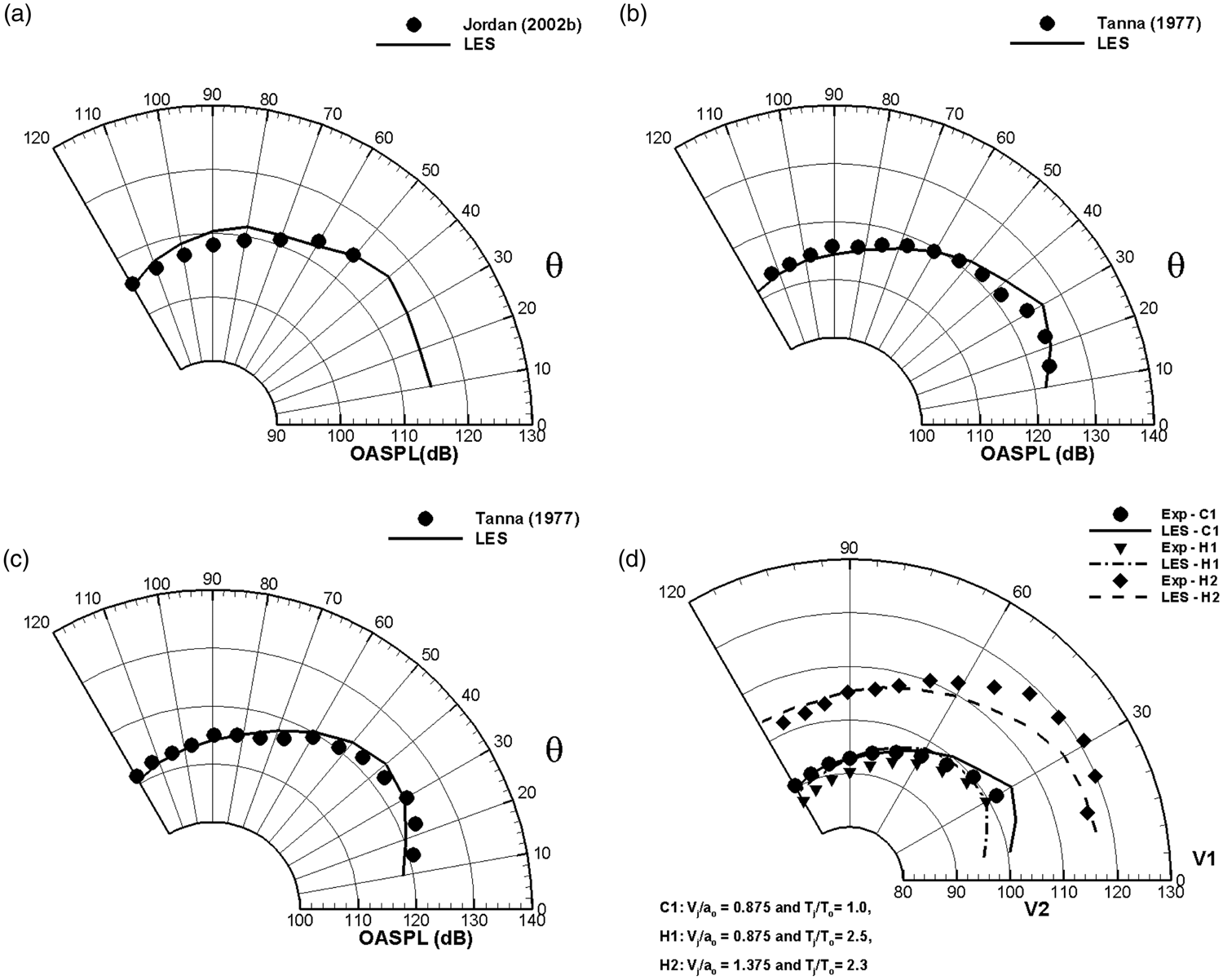

Figure 16 shows the sound pressure level (SPL) spectra for case 2 at $R = 100 D$ at three observer angles of $30 \deg, 60 \deg$ and $90 \deg$ . The LES spectra are in good agreement with the measurements. The current spectra are resolved up to Strouhal number $St ~ 2 - 3$ for the current grids.

Figure 16.

Sound pressure level (SPL) spectra for case 2 at R=100D, at (a) 30°, (b) 60° and (c) 90°.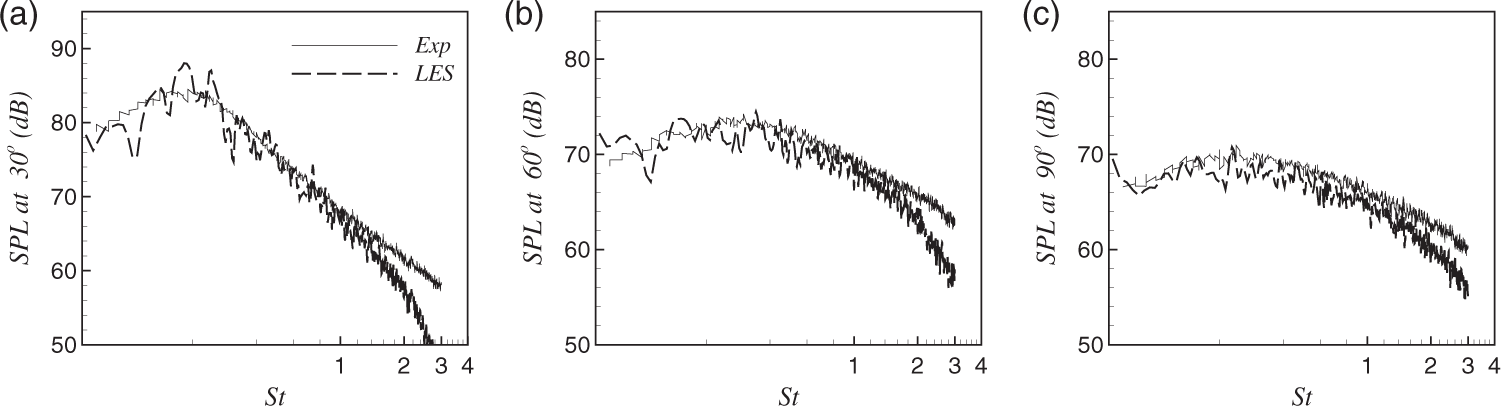

Conclusion

To validate a new simulation strategy, simulations were run for two different Mach numbers and also for two different mesh densities. Simulations for both cases were run at a Re lower than the rig Re, while maintaining the boundary layer state at the nozzle exit. A RANS layer was used over the full boundary layer thickness allowing tuning to rig conditions. The scaling of μ_t in the RANS model has successfully shown to conserve the rig Re for the Re dependent boundary layer region. The technique promises reliability for industrial scale simulations. The flow computation is able to predict peak turbulence levels reasonably well, thus showing the effectiveness of the scheme. The proposed method also eliminates the grid dependence of the solution. The farfield noise directivity gave encouraging match with measurements. This demonstrated usefulness of the proposed technique for noise computations.

Footnotes

Acknowledgements

We would to like thank Engineering and Physical Sciences Research Council (EPSRC) and United Kingdom turbulence consortium (UKTC) for the computational resources used for this study, on UK supercomputing facilities, ARCHER and HECToR under EPSRC grant EP/L000261/1. Some of the computations were also performed under PRACE award on HERMIT.

Declaration of conflicting interests

The author(s) declared no potential conflicts of interest with respect to the research, authorship, and/or publication of this article.

Funding

The author(s) disclosed receipt of the following financial support for the research, authorship, and/or publication of this article: The first author was supported by Dr Manmohan Singh Scholarship. Some of the work was funded in HARMONY and SILOET projects under the UK government TSB.

Appendix

References

Wilfert G, Sieber J, Rolt A, et al. 2007. New environmental friendly aero engine core concepts. In: ISABE, Beijing, China, 2–7 September 2007.

DeBonis

. Progress toward large-eddy simulations for prediction of realistic nozzle systems. J Propulsion Power 2007; 23: 971.

Eastwood

Tucker

. Hybrid LES-RANS of complex geometry jets. Int J Aeroacoustics 2011; 10: 661–686.

Bogey

Bailly

Juvé

. Noise investigation of a high subsonic, moderate Reynolds number jet using a compressible large eddy simulation. Theor Comput Fluid Dyn 2003; 16: 273–297.

Boersma

. Numerical simulation of the noise generated by a low Mach number, low Reynolds number jet. Fluid Dyn Res 2004; 35: 425–447.

Bogey C and Bailly C Investigation of subsonic jet noise using LES-Mach and Reynolds number effects. In: 10th AIAA/CEAS aeroacoustics conference, Manchester, UK, 10–12 May 2004.

Andersson N, Eriksson L and Davidson L LES prediction of flow and acoustic field of a coaxial jet. AIAA paper 2884, 2005, pp. 1–26.

Fayard B, Rahier G and Vuillot F. Modal analysis of jet flow from a coaxial nozzle with central plug. In: 15th AIAA/CEAS aeroacoustics conference, Miami, FL, 11–13 May 2009.

Andersson N, Eriksson L and Davidson L. A study of Mach 0.75 jets and their radiated sound using large-eddy simulation. AIAA paper 3024, 2004, p.2004.

10.

Bogey

Bailly

. Large eddy simulations of transitional round jets: influence of the Reynolds number on flow development and energy dissipation. Phys Fluids 2006; 18: 065101.

11.

Viswanathan

. Aeroacoustics of hot jets. J Fluid Mech 2004; 516: 39–82.

12.

Bodony D and Lele S Spatial scale decomposition of shear layer turbulence and the sound sources associated with the missing scales in a large-eddy simulation. AIAA Paper 2454, 2002.

13.

Ciardi

Sagaut

Klein

. A dynamic finite volume scheme for large-eddy simulation on unstructured grids. J Comput Phys 2005; 210: 632–655.

14.

Naqavi

Wang

Z-N

Tucker

. Far-field noise prediction for jets using large-eddy simulation and Ffowcs Williams-Hawkings method. Int J Aeroacoustic 2016; 15: 1–29.

15.

Eastwood

Tucker

Xia

. Large-eddy simulations and measurements of a small-scale high-speed coflowing jet. AIAA J 2010; 48: 963–974.

16.

Tucker

. Differential equation-based wall distance computation for DES and RANS. J Comput Phys 2003; 190: 229–248.

17.

Tucker

. The LES model’s role in jet noise. Prog Aerosp Sci 2008; 44: 427–436.

18.

Andersson

Eriksson

Davidson

. Investigation of an isothermal Mach 0.75 jet and its radiated sound using large-eddy simulation and Kirchhoff surface integration. Int J Heat Fluid Flow 2005; 26: 393–410.

19.

Bridges J and Wernet MP. Establishing consensus turbulence statistics for hot subsonic jets. In: 16th AIAA/CEAS aeroacoustics conference, Stockholm, Sweden, 7–9 June 2010.

20.

Tanna

. An experimental study of jet noise part 1: turbulent mixing noise. J Sound Vibr 1977; 50: 405–428.

21.

Shur

Spalart

Strelets

. Towards the prediction of noise from jet engines. Int J Heat Fluid Flow 2003; 24: 551–561.

22.

Eastwood

Xia

Tucker

. Large-eddy simulation of complex geometry jets. J Propulsion Power 2012; 28: 235–245.

23.

Eastwood S. Hybrid RANS-LES of complex geometry jets. PhD Thesis, University of Cambridge, Cambridge, 2009.