Characteristics of jet noise: A synthesis

Abstract

It is a distinct privilege to produce this article to honor Professor Tam, the foremost authority on jet aeroacoustics. The fundamental characteristics of jet noise have been studied for 70 years, since the pioneering work of Lighthill in the 1950s. The acoustic analogy, with many variants, has served as the leading theory for nearly 50 years. Many leading researchers in the 1970s formulated theories to interpret the measured trends from subsonic and supersonic jets, using acoustic analogy and flow features as the framework. Quadrupoles, dipoles and monopoles were believed to constitute the sources of noise. The discovery of large-scale organized structures in free shear layers and jets sparked a different avenue of thinking about their importance for noise generation. Tam was the first to clearly demonstrate that these structures are efficient generators of noise and constitute the dominant noise sources, especially in the downstream direction. Now, two schools of thought emerged on the sources of jet noise. Experimental measurements showed that the mean flow as well as the turbulence statistics exhibit a self-similarity in the mixing layer and another similarity in the fully developed jet. Based on these observations, Tam proposed that since noise is generated by the turbulence of the jet, the noise spectra generated by fine-scale and large-scale turbulence should also exhibit self-similarity. By examining a large set of supersonic jet noise data acquired at NASA Langley, Tam offered evidence that the turbulent mixing noise of high-speed jets does consist of two independent self-similar components. In this paper, experimental evidence is compiled from an extensive database that quantifies the effect of several parameters that affect jet spectra. A new scaling method is developed and extended to noise predictions for realistic dual-stream nozzle geometries. The objectives of this paper are to serve as a synthesis of noise characteristics and to focus on application to real-world problems. Results from five different experimental measurements are examined: (1) farfield spectral characteristics; (2) azimuthal and polar correlations in the farfield; (3) correlations of jet turbulence fluctuations and farfield sound; (4) measurement of source distributions with an elliptic mirror; and (5) space-time correlation measurements in the nearfield with a cage array, and nearfield-farfield correlations. Two distinctly different trends are observed in the angular ranges of 50° – ∼120° and ∼120° – 165° for all the parameters investigated with the above five approaches. The salient observations are mutually supporting, and the cumulative weight lends credence to the proposition that there are two distinct sources of turbulent mixing noise.

Keywords

Jet noise turbulent mixing noise noise measurements noise sources modeling and prediction

Introduction

The dawn of the age of turbojet engines began in the 1930s. Subsequent introduction into service for military aircraft in the 1940s drew attention to the unwanted annoyance of high noise levels. It became abundantly clear that major advances in noise reduction would be necessary, before widespread acceptance and application for commercial service. Intense research in the following decades led to turbofan engines of increasing bypass ratios, with attendant noise reduction and enhanced propulsive efficiency, thereby making them the dominant propulsion system since then. Experimental investigations in the early years provided information on the scaling of jet noise and guidance for theories for the generation and radiation of jet noise. The pioneering work of Lighthill^1,2 heralded the field of jet aeroacoustics and sparked major interest in the measurement, scaling, modeling and prediction of jet noise. Lighthill’s acoustic analogy has been the dominant theory of jet noise for several decades. The acoustic analogy established the eighth power dependence on jet velocity of the radiated sound power, and the high and low frequency dependencies of the jet spectra. Since the formulation of the acoustic analogy, there have been several theoretical developments and variants of the basic theory: see Proudman,³ Philips,⁴ Doak,⁵ Ffowcs-Williams,⁶ Ribner,⁷ among others. Lilley⁸ developed an acoustic analogy that explicitly accounted for the effects of the mean flow on the radiated noise. For a detailed and masterful exposition of these early jet noise theories, see Lilley.⁹ This paper is not meant to serve as a review of all the past studies: as such, only sample references are cited here, insofar as to highlight key topics and the main findings.

The author’s work has focused mainly on experimental research; it has encompassed both fundamental aspects as well as practical applications. As a researcher in the aerospace industry, it has been a vital objective to develop prediction methods that can be used readily for absolute spectral evaluations for actual modern turbofan engines that power aircraft today. However, this endeavor would not be possible without obtaining a clear understanding of the underlying and intrinsic characteristics of jet noise, first for simple single-stream jets and systematically progressing to representative and realistic dual-stream nozzle exhaust geometries. The results reported here build upon the vast body of knowledge gained and accumulated by numerous experts in the last 70 years. My own investigations have been informed and influenced by personal interactions with many leading lights in the field, who provided much inspiration. The author would like to take this opportunity to thank all of them.

The objectives of this paper are as follows: (1) highlight the contributions of Professor Tam in advancing overall understanding of the many features of jet noise; (2) use the author’s own jet noise database to bolster and expand the original observations of Professor Tam; (3) gather and collate the significant findings from the above database in one place (from several publications); (4) quantify the effect of parameters that could influence jet spectra, such as Reynolds number, jet temperature, initial conditions, etc.; (5) describe new scaling laws without invoking arbitrary assumptions; and (6) highlight the development of methods for direct absolute spectral predictions at all angles, first for single-stream jets, and then for realistic nozzle exhaust geometries of turbofan engines. As already stated, the emphasis is on practical applications vis-à-vis airplane noise certification, which represents the culmination of fundamental research. The equally important consideration of noise reduction is not covered here, as it is beyond the scope of this article.

Discovery of large coherent structures and their importance for noise

Turbulent flows were observed in the 1960s to be more ordered than had been believed previously. For the round jet, Mollo-Christensen¹⁰ was one of the first to report such a finding. This was followed in the early 1970s by Crow and Champagne¹¹ and Brown and Roshko¹²; they reported the observation of large coherent structures in turbulent jets and free shear layers. These structures were perceived as wave-packets. The intimate connection between stability and noise generation predates the discovery of these structures; see Mollo-Christensen and Narasimha,¹³ Batchelor and Gill,¹⁴ Mollo-Christenson,¹⁰ Michalke,¹⁵ Bishop, Williams and Smith,¹⁶ among many others.

It is now widely established that the turbulence in free shear layers is not completely random but more coherent and orderly, and turbulent flows contain both fine-scale and large-scale structures. Both fine-scale (uncorrelated) turbulence and large-scale turbulence generate noise. The coherent large-scale structures have been modeled as instability waves and their importance in noise radiation has been recognized, as noted. For supersonic jets, and subsonic jets at high temperatures as in practical jet engine applications, the large-scale structures propagate downstream at supersonic speeds relative to the ambient speed of sound. Though many researchers had suggested/hypothesized a possible link between instability waves and noise radiation, Tam¹⁷ was the first to clearly demonstrate that these structures are efficient generators of noise and constitute the dominant noise sources, especially in the downstream direction. There have been several experimental and theoretical developments related to the measurement and modeling of the source mechanisms associated with the large-scale structures: Tam,¹⁸ Chan and Westley,¹⁹ Morris,^20,21 Liu,²² Tam,²³ McLaughlin, Morrison and Troutt,²⁴ Ffowcs Williams and Kempton,²⁵ Morris and Tam,²⁶ Tam and Morris,²⁷ Seiner, McLaughlin and Liu,²⁸ Tam and Burton,²⁹ Tam, Chen and Seiner,³⁰ to name just a few. Tam and Burton,²⁹ by means of a matched asymptotic expansion solution, provided a detailed description of the physical mechanism by which supersonically propagating large-scale structures/instability waves generate noise. A comprehensive treatment of the role of the large turbulence structures in the generation of the turbulent mixing noise as well as the broadband shock-associated noise is given by Tam.^31–33

There are three components of jet noise; turbulent mixing noise is present for all jets. Two other components manifest themselves for imperfectly expanded supersonic jets; these are the broadband shock-associated noise and discrete screech tones. Broadband shock-associated noise is beamed towards the lower inlet angles, whereas turbulent mixing noise is radiated principally to large aft angles, close to the jet axis. The intensity of the shock-associated noise is dependent on the degree of mismatch between the design Mach number M_d and the fully expanded jet Mach number M_j. The relative importance of the broadband shock-associated noise and the turbulent mixing noise is a strong function of the radiation angle and the jet operating conditions. Throughout this paper, the polar angle is measured from the jet inlet. Let us first examine the polar directivity of the overall sound pressure level (OASPL) for the F-404 engine that powers the F-18 tactical fighter aircraft. Figure 1 from Viswanathan and Czech³⁴ shows the directivity of the overall sound pressure level (OASPL) for typical nozzle geometry at typical takeoff power, referred to as military (MIL) power here. Two sets of data, one obtained at static conditions and the other at a flyover Mach number of 0.233 are shown. For the static case, the peak level at ∼130° is ∼ 15 dB higher than those at the lower radiation angles, where shock-associated noise is dominant. Note that the turbulent mixing noise is the dominant component in the peak radiation sector in the aft quadrant. For the case with forward flight, the difference in level is still roughly 12 dB. The reduction in the mixing noise level due to forward flight is seen to be ∼ 4 dB at the peak angles.

Figure 1.

Directivity of the overall sound pressure levels at MIL power. Flight Mach numbers of 0.0 and 0.233.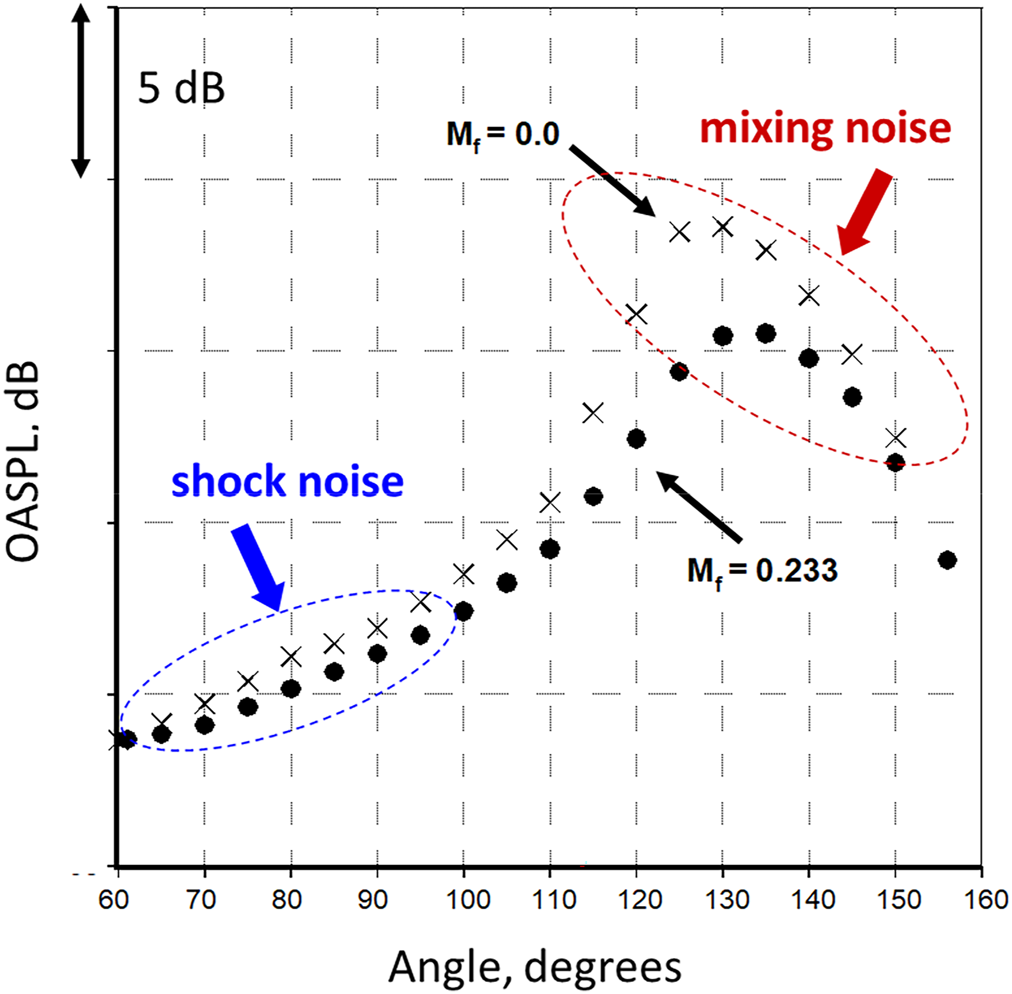

The choice of an actual engine operated at realistic over-expanded nozzle pressure ratio serves a vital purpose of assessing the relative importance for a real-world problem. The main message from this figure is the following: the mixing noise in the peak radiation sector must be reduced to mitigate the noise impact of even fighter aircraft. All turbofan engines that power commercial aircraft are operated at subsonic jet Mach numbers at takeoff. Therefore, turbulent mixing noise is the chief component of interest. Consequently, the main focus of this paper is on this component.

Identification of two similarity spectra

Experimental measurements have shown that the mean flow as well as the turbulence statistics exhibit a self-similarity in the mixing layer and another similarity in the fully developed jet. Based on these observations, Tam and Chen³⁵ and Tam, Golebiowski and Seiner³⁶ proposed that since noise is generated by the turbulence of the jet, the noise spectra generated by fine-scale and large-scale turbulence should also exhibit self-similarity. By examining a large set of supersonic jet noise data acquired at NASA Langley, Tam offered evidence that the turbulent mixing noise of high-speed jets does consist of two independent self-similar components. These were termed the fine-scale similarity (FSS) spectrum and large-scale similarity (LSS) spectrum. The relative contributions of these two noise sources are dependent on the jet Mach number, the jet temperature, and the radiation angle. The FSS spectrum has a broad peak and a slow roll-off at the lower and higher frequencies, away from the peak. The LSS spectrum has a narrower peak and a sharp roll-off at lower and higher frequencies; thus, they are distinctly different. The identification of the similarity spectra was a major achievement, based on the idea of the jet turbulence containing both small-scale (random) structures and large-scale organized structures, and both of them emitting noise. This original finding is on par with the demonstration of noise radiation by large-scale structures by Tam.^17,18

The analysis of Tam, Golebiowski and Seiner³⁶ was restricted to single-stream supersonic spectra obtained at NASA Langley’s Jet Noise Laboratory and unheated subsonic jets. Viswanathan³⁷ carried out an in-depth analysis of the similarity spectra and examined the spectral shapes of subsonic heated jets and those from dual-stream nozzle geometries. He also pointed out some shortcomings in the determination of the exact similarity shapes; however, these minor quibbles in no way detract from Tam’s seminal findings. Figure 2 shows measured spectra in the polar angular range of 90°–150°, from a heated jet at a Mach number of 1.0 and total (stagnation) temperature ratio of 3.2. Also presented in this figure are comparisons of the data with the FSS or LSS empirical spectra. There is excellent agreement between the measured spectra and the FSS shape at all the angles from 90° to 110°. The same trend prevails for spectra at lower inlet angles (not shown here). As we move aft, the spectral shape begins to change and gets peakier. The contribution from the large-scale structures becomes pronounced and there is gradual transition from the FSS to the LSS shape, which prevails at a polar angle of 150°. Note that the data in the intermediate angular range of ∼120° to ∼140° cannot be characterized by either of the empirical spectrum by itself, indicating that there is varying levels of contributions from the two sources. Viswanathan³⁷ also provided evidence from the analysis of noise from dual-stream nozzles that the measured spectra in the forward quadrant and near-normal angles conform to the shape of the fine-scale spectrum, regardless of nozzle geometry and operating conditions. This feature was seen even for inverted velocity profile jets, jets from mixer-ejectors, elliptic jets, etc. Therefore, the FSS shape is universal. The small-scale turbulence, at Kolmogorov scale, is nearly universal except in the near-wall viscous region. It stands to reason then, that the spectrum of the noise generated should also be universal in shape. Tam and Auriault³⁸ developed a semi-empirical theory capable of predicting the fine-scale turbulence noise from cold to moderate temperature jets. Tam, Pastouchenko and Viswanathan³⁹ extended this semi-empirical theory to high-temperature jets of present day commercial engines. Good spectral agreement between the predictions and data was obtained in the angular range of 50° to 110°, for a wide range of Mach numbers from 0.6 to 2.0, and total temperature ratios up to 3.2. See these two references for more details.

Figure 2.

Comparison of data with similarity spectra. M = 1.0, T_t/T_a = 3.2. Symbols: data; solid lines: FSS; dashed: LSS.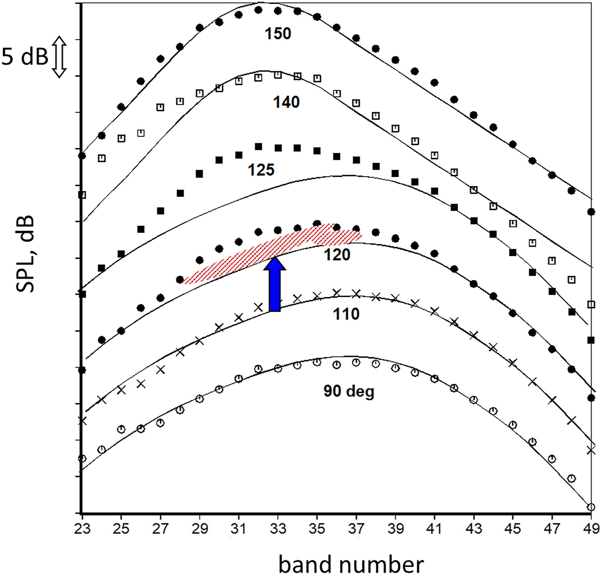

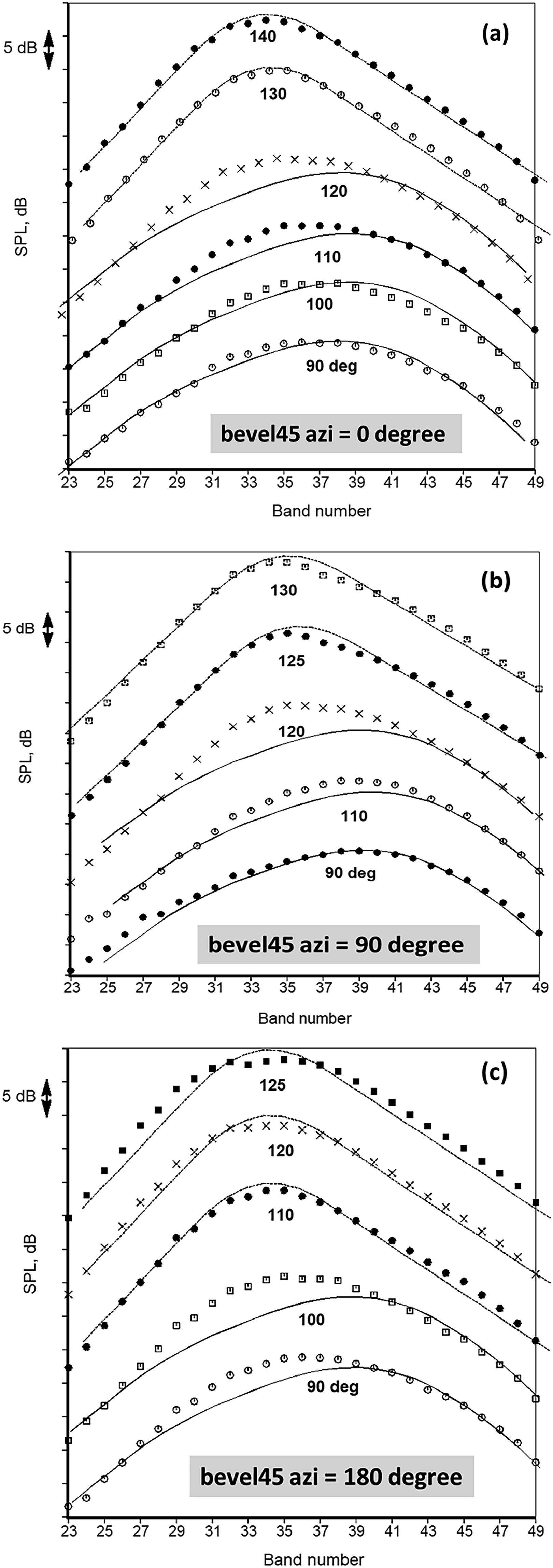
The picture for the LSS shape is more nuanced, as there is not a single fixed shape at large aft angles. This point will be reinforced with concrete examples in the following sections. Viswanathan⁴⁰ demonstrated that the basic noise radiation pattern observed for round nozzles could be modified with a simple beveled nozzle; by doing so, noise reduction could be achieved in the direction of the ground. Figure 3 shows a conceptual sketch of the beveled nozzle and the measurement conventions for the bevel as well as the azimuthal angles. Detailed aeroacoustic measurements were performed on two nozzles of different bevel angles. Noise measurements, over a wide range of polar angles, were made at several azimuthal angles to map the azimuthal variations. Figure 4 shows spectral variations for the same jet operating conditions as for the round nozzle in Figure 2: M = 1.0, and T_t/T_a = 3.2. For the bevel45 at an azimuthal angle of 0° (4a), the measured spectra start deviating from the FSS shape at a lower polar angle of ∼120° and a LSS shape is observed at a polar angle of 130°. As we go around the periphery of the beveled nozzle to an azimuthal angle of 90° (4b), we notice that the LSS shape is seen for the spectra at a polar angle of 125° and higher. At an azimuthal angle of 180° (4c), the spectral characteristics are dramatically different from those for the round nozzle. Even at 90° there is a slight hump near the peak; at 100° this hump is more pronounced and there is major deviation from the FSS shape. The most surprising feature is the observation of the LSS shape for the measured spectra at a polar angle of 110°.

Figure 3.

Conceptual sketch of the beveled nozzle and the measurement convention for the bevel angle, the polar angle (χ) and the azimuthal angle (ϕ).

Figure 4.

Comparison of data with similarity spectra. M = 1.0, T_t/T_a = 3.2. Symbols: data; solid lines: FSS; dashed: LSS. (a) bevel45, azi = 0°; (b) bevel45, azi = 90°; (c) bevel45, azi = 180°.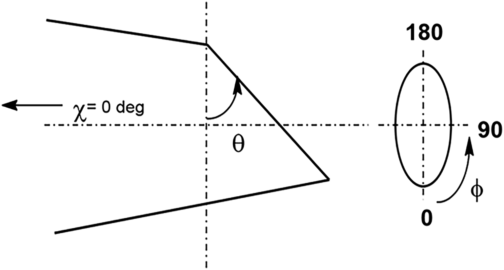

It is generally accepted that the large-scale structures do not radiate noise at an angle of 90°. Figure 5 presents spectra at three Mach numbers of 0.6, 0.7 and 1.0 at a polar angle of 90°. When we examine the spectra, it is obvious that the FSS shape by itself does not fit the measured data even at a low Mach number of 0.6. The LSS component must be added, as shown symbolically, to fit the spectral peak. For a round nozzle, the angular sector where both components are significant occurs at much larger polar angles. In fact, for the beveled nozzle one would have to be at a very low angle of 60 deg to recover the FSS shape, as shown in Figure 24 in Viswanathan.⁴⁰ Therefore, it is obvious that the radiation pattern has been completely altered with the above concept. First of all, the noise generated by the large-scale structures, which is beamed preferentially to angles close to the jet axis for a round nozzle, is radiated to lower polar angles for a beveled nozzle. Of greater significance is the fact that this component is radiated towards the azimuthal direction with the shorter side of the beveled nozzle. With the longer lip of the beveled nozzle at the bottom-dead-center, this means that the noise is radiated up into the sky. Additional evidence to underpin the above statements will be provided in a later Section on the “Evidence for Two Sources.”

Figure 5.

Comparison of data with the similarity spectra. Bevel45, T_t/T_a = 3.2, polar angle = 90°, azi = 180°. Symbols: data; solid lines: FSS; dashed: LSS.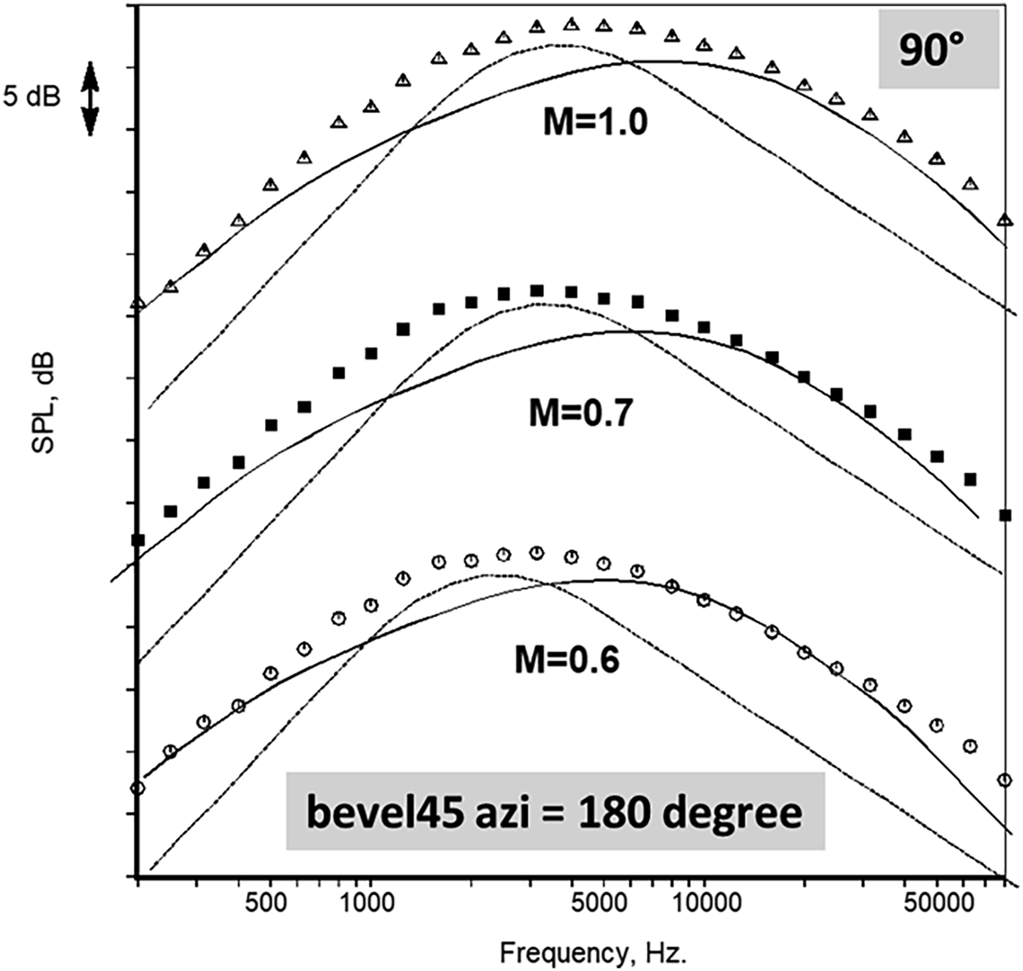

Viswanathan³⁷ showed clearly that the spectral shape associated with the large-scale structures of single jets does not characterize the noise of dual-stream jets at large aft angles. There are multiple sources of noise; the secondary shear layer between the fan flow and the ambient flow is responsible for the generation of high-frequency noise. When the primary jet velocity is increased with fixed secondary plenum conditions, there is an increase in spectral levels only at the lower frequencies. That is, there is a major change in spectral shape. It is not implied or suggested that the noise from large-scale structures is not important for dual-stream jets; rather, it is not possible to identify it through just an examination of the spectral shape.

Now there is spectral indication that these two distinct shapes prevail for unheated and heated subsonic and supersonic jets. The noise signatures could be generated by different mechanisms: that is, the jet turbulence (random and organized) constitutes the sources of jet noise. Tam⁴¹ provides a review of this viewpoint, with emphasis on the flow physics of turbulence and the mechanisms of noise generation. This is a radical departure from the classical theories of jet noise. Viswanathan⁴² carefully examined the tenets of the classical theories of jet noise with his own database and showed that there is no experimental evidence for the main classical ideas of jet noise, as consisting of quadrupoles, dipoles and monopoles, and moving sources, as they are inconsistent with the data. The notions of flow/acoustic interaction, Doppler frequency shift, and convective amplification are also tenuous; see Sections “Effect of Reynolds number on jet noise” and “Effect of temperature on jet noise” below for detailed treatment of these hypotheses. The idea of two distinct sources that are related to the fine-scale and large-scale turbulence of the jet plume was also investigated. Experimental evidence to support the latter proposition is presented in a later Section. Morris and Viswanathan⁴³ present a more balanced view of these disparate ideas of noise sources and delve into the potential reasoning behind the initial thinking. As emphasized by Viswanathan,⁴² even the brightest researchers are not immune to being misled by incorrect or ambiguous trends seen in the poor quality of the data obtained in the past. Advances in electronics, instrumentation and experimental techniques have led to better data, which in turn have enabled the evolution of more consistent theories.

All the above investigations and the salient observations on large-scale structures vis-à-vis noise generation have been restricted to high-speed jets, with supersonic convective velocities. For subsonic jets, especially at low and moderate temperatures, the large turbulence structures propagate downstream at subsonic speeds relative to the ambient speed of sound. We address the issue of the noise contribution from these structures even at low jet velocities in a later section.

Experimental program and results

Numerous experimental campaigns have been carried out over 15 years by the author, and a vast database of jet noise has been acquired for (1) single-stream jets, (2) dual-stream jets with separate flows, (3) dual-stream jets with internal mixers and a confluent common nozzle, (4) rectangular mixer-ejectors, and (5) a variety of novel geometries. The author had the good fortune to work for Boeing, with access to an extremely large aeroacoustic wind tunnel facility and the support of dedicated laboratory personnel with deep institutional knowledge and expertise. Furthermore, the author benefited from the available databases from static engine tests and airplane flyover tests, accumulated over 50 years of full-scale testing. For the sake of completeness, a short description of the Low Speed Aeroacoustic Facility (LSAF) is first included.

Boeing designed and built a jet simulator in the early 1990s, referred to as the NTL3800 rig. The jet rig consists of high-temperature supply piping, burners, instrumentation, and aerodynamic fairings designed for a high flow capability of 20 lb/s (9.07 kg/s) in single flow mode and 30 lb/s (13.61 kg/s) in dual-flow mode, for continuous operation. Both of the streams may be heated to 1950°R (1083 K) to simulate inverted-velocity-profile jets, if desired. The centerline of the jet simulator is 17.2 ft (5.3 m) above the ground. Several polar microphone arrays are usually installed on poles; these include both fixed-distance straight-line arrays and a 25-foot circular array. The polar angular range covers 50° to 160°. The origin of the coordinate system is located on the jet centerline, at the nozzle exit plane. The rig also has provision to control the external boundary-layer growth. A vacuum system with two perforated sections is located upstream of the model. Suction through the perforated skin allows the thickness of the external boundary layer to be controlled. This jet rig is integrated with a six-component force balance, referred to as the E-3 balance. A photograph of the anechoic facility is shown in Figure 6; the jet simulator is embedded in an open-jet wind tunnel, which can provide a maximum free-stream Mach number of 0.32. Both acoustic and thrust measurements are made simultaneously. The anechoic chamber is large enough to accommodate several diagnostic tools and ensures measurements in the true farfield of the sources. The six-component balance can pass two airflow lines, fuel flow lines, and a vacuum line for the control of the boundary layer, across the balance plane. The support structure for the balance and a service module (that routes instrumentation and control cables, fuel and hydraulic lines) are mounted on air bearings and may be placed anywhere within the anechoic chamber. All air lines, fuel lines and instrumentation are contained within an aerodynamic strut. This strut has provisions for all the lines to be passed across the balance interface in a manner that avoids interference with force measurements.

Figure 6.

Photograph of the Low Speed Aeroacoustic Facility (LSAF).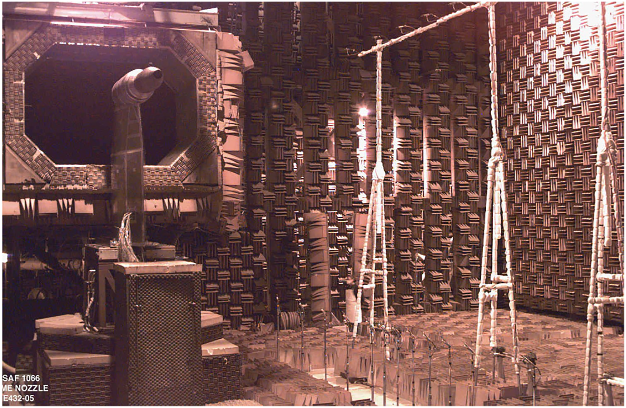

Bruel and Kjaer Type 4939 microphones (newer type that replaced Type 4135) are used for free field measurements. The microphones are set at normal incidence and without the protective grid, which yields a flat frequency response up to 100 kHz. Narrowband data with a bin spacing of 23.4 Hz are acquired and synthesized to produce one-third-octave spectra, up to a center band frequency of 80,000 Hz. The cut-off frequency for the anechoic chamber is well below 200 Hz. Spectra in the range of 200 Hz to 80,000 Hz are used in the analyses. The as-measured data are corrected to a common distance of 20 feet (6.096 m) from the center of the nozzle exit (coordinate system with origin at the center of the nozzle exit) and lossless conditions. The atmospheric attenuation coefficients are obtained from the method of Shields and Bass.⁴⁴ Implicit in this process is the assumption of linear propagation, with the sound pressure level obeying the (1/r²) dependence. The normalization process may be written as,

S P L_{(20 f e e t)} = S P L_{m e a s u r e d} - 10 Log_{10} {(\frac{20}{r})}^{2} + r [A A_{(t e s t d a y)}]

(1)

where r (ft) is the distance of the microphone from the origin of the coordinate system, [AA] are the atmospheric absorption coefficients (which are frequency dependent) per foot. The above equation provides spectra corrected to lossless conditions; lossless spectra are presented throughout this paper. The accuracy of the weather corrections and the suitability of the different proposed methods have been evaluated; it was shown that the method of Shields and Bass⁴⁴ was the best at the higher frequencies of interest in model scale tests

A major effort over several years was carried out to refurbish the jet rig, instrumentation systems, and establish good test practices for the acquisition of high-quality acoustic data, free from extraneous noise contamination. Significant improvements to flow uniformities, both in pressure and temperature distributions inside the supply duct, were first achieved so as to enhance the fidelity of setting up the proper nozzle operating conditions; see Figures 3 and 4 in Viswanathan.⁴⁵ Complete details on the efficacies of these actions may be found in Viswanathan.^45–47

Aeroacoustic data have been obtained at seven stagnation temperature ratios (T_t/T_a) of 1.0, 1.8, 2.2, 2.7, 3.14, 3.2 and 3.51 for the basic database, at fixed Mach numbers of 0.3, 0.4, 0.5, 0.6, 0.7, 0.8, 0.9, 1.0, 1.23, 1.36, 1.47 and 1.56. Data at additional plenum conditions were also acquired to resolve specific issues (fixed static temperature ratios, different nozzle contours, fixed jet velocities, etc.) as described throughout this paper. A variety of nozzles (mainly conical), with different diameters (D) of 1.5″ (3.81 cm), 2.45″ (6.22 cm), 3.46″ (8.8 cm), 4.21″ (10.69 cm), 4.71″ (11.96 cm), 4.9″ (12.44 cm), 5.34″ (13.56 cm) and different internal contours were used in the generation of the aeroacoustic database. The high flow capacity of the rig and a very large anechoic chamber enable the testing of large nozzles, which is essential for engine/airplane applications.

The good spectral quality is first demonstrated with a single plot in Figure 7. Lossless spectra from the above nozzles at a jet stagnation temperature ratio of 2.2, with Mach numbers of 0.5, 0.6, 0.7, 0.8, 0.9 and 1.0 have been normalized for noise per unit area (conveniently taken to be one square inch), through the subtraction of [10*Log₁₀(A), where A is the nozzle exit area]. A polynomial curve-fit is also shown. A velocity scaling, which is explained in a later section, has also been applied to the data. Thus, the parameter on the y-axis represents normalized spectra, plotted against the Strouhal number on the x-axis. It is recognized and acknowledged that this figure is out of sequence; however, this figure encapsulates and illustrates the data quality using the most stringent criterion. The spectra from more than 20 individual and independent measurements form one smooth curve. If there is internal noise contamination, it would be readily evident, as it would have a more severe impact with higher mass flows needed for the larger nozzles, especially at low Mach numbers. Obviously, that is not the case. Therefore, there should be no issues with the experimental findings and results reported in this article.

Figure 7.

Spectral collapse from six different nozzles of various diameters and jet Mach numbers. T_t/T_a = 2.2.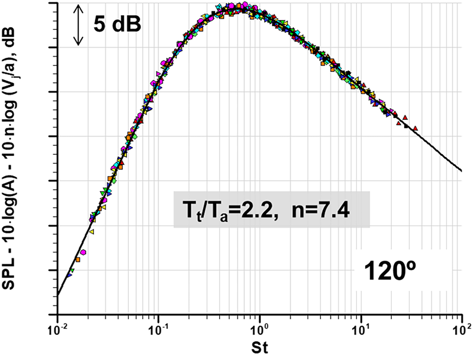

As clearly stated in the list of objectives, many of the results presented here are not entirely new. Rather, they are a recapitulation and compilation of the major characteristics of jet noise and meant to serve as a synthesis. Viswanathan^42,45,48 examined the quality of data from several major facilities and pointed out they were unreliable for extracting the finer effects and in formulating theoretical explanations. Therefore, the current database serves as the basis for most of the observations.

Lilley⁹ has this closing remark in his review article: “Finally, the importance of good, reliable, and accurate experimental data in all studies of aerodynamic noise is stressed. At best the theoretical work can only assist in providing a suitable framework in which to analyze the results and the presentation of the experimental data for prediction purposes.” This truism is timeless and always worth remembering.

Effect of Reynolds number on jet noise

Viswanathan⁴⁸ first uncovered an unexpected effect of Reynolds number on jet noise. The material presented in this section is taken mainly from this paper. The noise from heated jets has been measured since the early seventies by several researchers, both in Europe and in the USA. A careful examination of the available data reveals that the database is by no means comprehensive and that the quality of the data is not uniformly high. Measurement of noise at low jet velocities (V_j/a ≤ 0.5, where a is the speed of sound in ambient air) poses a daunting challenge since the magnitude of the contamination could be much higher than the jet noise level. Many fundamental questions on the noise of hot subsonic jets still remain unanswered, even after decades of study. For example, it has been believed widely by jet noise theoreticians that an extra source of noise, of the dipole type, is important at high temperatures, especially at low Mach numbers. The effects of Reynolds number of scale-model nozzles are rarely appreciated or investigated thoroughly. This study addressed these and several other issues. The effect of Reynolds number is evaluated through testing nozzles of different diameters at the same jet operating conditions. Comparisons of these data, properly scaled, would uncover the effect of the Reynolds number explicitly.

Three nozzles with conical contractions and shallow cone angles have been utilized to establish the effect of Reynolds number; the diameters are 1.5″, 2.45″ and 3.46″, respectively. The plenum conditions are fixed; there is lengthy axial section for the boundary layer to develop and become turbulent at the nozzle exit plane. The spectral shape of unheated jets is now presented. Figure 8 shows a comparison of the measured spectra (D = 1.5″) at 90° and the fine-scale similarity (FSS) spectrum of Tam et al.,³⁶ from unheated jets at several Mach numbers of 0.3, 0.4, 0.5, 0.6, 0.7, 0.8, 0.9, and 1.0. The curves have been spaced apart to enhance visual observation and the maximum spectral level associated with each curve is noted in all the figures. The peaks of the similarity spectra are placed on top of the peaks of the measured spectra in the following figures. There is excellent agreement for Mach numbers 0.6 and higher. However, at a Mach number of 0.5, the data at the highest frequencies are slightly higher than the empirical curve. At M = 0.4, the discrepancy is more pronounced and the spectrum starts deviating above a frequency of 20,000 Hz (band # 43, where band # = 10 × Log₁₀ (f), f is frequency in Hz.). The spectrum for M = 0.3 does not resemble that of jet noise at all and is corrupted completely by rig noise.

Figure 8.

Comparison of spectra from unheated jets. D = 1.5 inch, angle = 90°. Symbols: M = 0.3, 0.4, 0.5, 0.6, 0.7, 0.8, 0.9, 1.0; lines: FSS spectrum.

Let us now examine the effect of temperature on jet noise. The measured spectra at 90° (D = 1.5″) at various temperatures (T_t/T_a = 1.0, 1.8, 2.2, 2.7, 3.2) are shown for a M = 0.6 jet in Figure 9. Also shown in these figures are comparisons with the fine-scale similarity spectrum. Again, the curves have been spaced apart to enhance visual observation and do not reflect the noise increase due to heating. As can be seen, when the jet is heated at these low Mach numbers, the spectral shape changes. For the unheated case there is excellent agreement with the FSS spectrum, as seen in Figure 8. However, for the heated cases, the peak frequency shifts to lower values and there is an extra hump near the peak, which is more pronounced at the higher temperatures.

Figure 9.

Comparison of measured spectra with fine-scale similarity spectrum. M = 0.6, angle = 90°, D = 1.5”. •: T_t/T_a = 1.0; Δ: T_t/T_a = 1.8; o: T_t/T_a = 2.2; x: T_t/T_a = 2.7; □: T_t/T_a = 3.2.

Many researchers in the past have proposed that the source of jet noise consists of quadrupoles and dipoles, with the contributions of dipoles pronounced at high jet temperatures, see for example Figure 8 in Fisher, Lush and Harper Bourne.⁴⁹ Based on observations similar to those seen in Figure 9 here, from data obtained by Tanna, Dean and Fisher,⁵⁰ Tanna⁵¹ and others, Tester and Morfey⁵² and Morfey, Szewczyk and Tester⁵³ developed master spectra for the noise generated by quadrupole and dipole sources. The diameter of the nozzle in the above experiments was 2.0 inches. For cold and isothermal jets, the noise was modeled as being dominated by quadrupole sources. The additional noise caused by the effect of heating the jet was then represented by temperature-fluctuation terms of dipole order. The master spectra for the quadrupole and dipole sources at 90°, where convection and refraction effects are minimal, had different shapes, with the peak frequency for the dipole term lower than that for the quadrupole term. The dipole spectrum moves up and down relative to the quadrupole spectrum, according to (a) the difference in density between the jet and the ambient air, and (b) the jet velocity ratio (V_j/a). Many in the jet noise community have accepted this view of the noise generation mechanisms for hot jets; see for example Goldstein.⁵⁴

Let us now see if there is an alternative explanation. The spectra shown in Figure 9 are now acquired with larger nozzles. Figure 10(a) and (b) show similar comparisons between the measured spectra and the FSS spectrum for a Mach 0.6 jet (D = 2.45″) at two angles of 70°, 90°, respectively. Let us concentrate our attention near the peak frequency. There is excellent agreement with the FSS spectrum and the spectral shape does not change even at the higher temperatures! The humps seen in Figure 9 are either completely absent or only barely discernible at the two higher temperature ratios at the two angles shown. Similar trends are observed at other Mach numbers as well. Additional evidence is provided in Viswanathan⁴⁸ with an even larger nozzle. Once again, the agreement with the FSS spectrum is very good at the higher temperatures and there is no change in spectral shape due to heating.

Figure 10.

Comparison of measured spectra with fine-scale similarity spectrum. M = 0.6, D = 2.45”. Δ: T_t/T_a = 1.0; o: T_t/T_a = 1.8; x: T_t/T_a = 2.2; •: T_t/T_a = 2.7; □: T_t/T_a = 3.2. (a): 70°; (b) 90°.

Figure 11 summarizes the above findings and brings out the effect of Reynolds number explicitly. The spectra at 90° from a jet of Mach number 0.7 and temperature ratio 3.2 from three nozzles of diameters 1.5″, 2.45″ and 3.46″ and comparisons with the FSS spectrum are shown. The extra hump is obvious in the spectra obtained with the smallest nozzle (D = 1.5″). The magnitude of the discrepancy between the data and the similarity spectrum near the spectral peak decreases for the nozzle with D = 2.45″ and almost completely disappears for the largest nozzle. The only parameter different in the three cases is the Reynolds number, with values of 204 000, 333 200 and 470 600 for the three nozzles, respectively.

Figure 11.

Comparison of measured spectra with fine-scale similarity spectrum. M = 0.7, T_t/T_a = 3.2, angle = 90°. x: D = 1.5”; •: D = 2.45”; o: D = 3.46”.

It is recognized that this method of identifying the hump through comparison with the FSS is somewhat subjective. However, this issue is put on a firmer footing as follows. First of all, the effects of jet velocity (V_j/a) and nozzle diameter are scaled out from the spectra. Specifically, the variation of the normalized spectra with Strouhal number is examined. An exponent of 5.53 has been obtained for the velocity dependence at 90°, as discussed in a later section on scaling. The normalized spectra are presented in Figure 12. The spectra obtained with the smaller nozzle (D = 1.5″) and denoted by the open symbols collapse to a single curve. The spectra for the larger nozzle (D = 3.46″) and denoted by the closed symbols, collapse onto a different curve. The biggest difference between these two families of curves occurs near the spectral peak and at Strouhal numbers slightly lower than the peak, with the normalized levels being higher for the smaller jet. This trend, suggested by humps for the smaller nozzle and no humps for the larger nozzle, shows up clearly when the spectra are compared on a common basis. Figure 17 in Viswanathan⁴⁸ shows the comparison of the Overall Power Level (OAPWL) at several Mach numbers from 0.5 to 1.24 for jets at T_t/T_a = 3.2, obtained with two nozzles of diameters 1.5″ and 2.45”. The levels obtained with the smaller nozzle are higher for all subsonic Mach numbers, reflecting the trend observed in Figures 11 and 12.

Figure 12.

Comparison of normalized spectra. T_t/T_a = 3.2, angle = 90°. Open symbols: D = 1.5”; closed symbols D = 3.46”.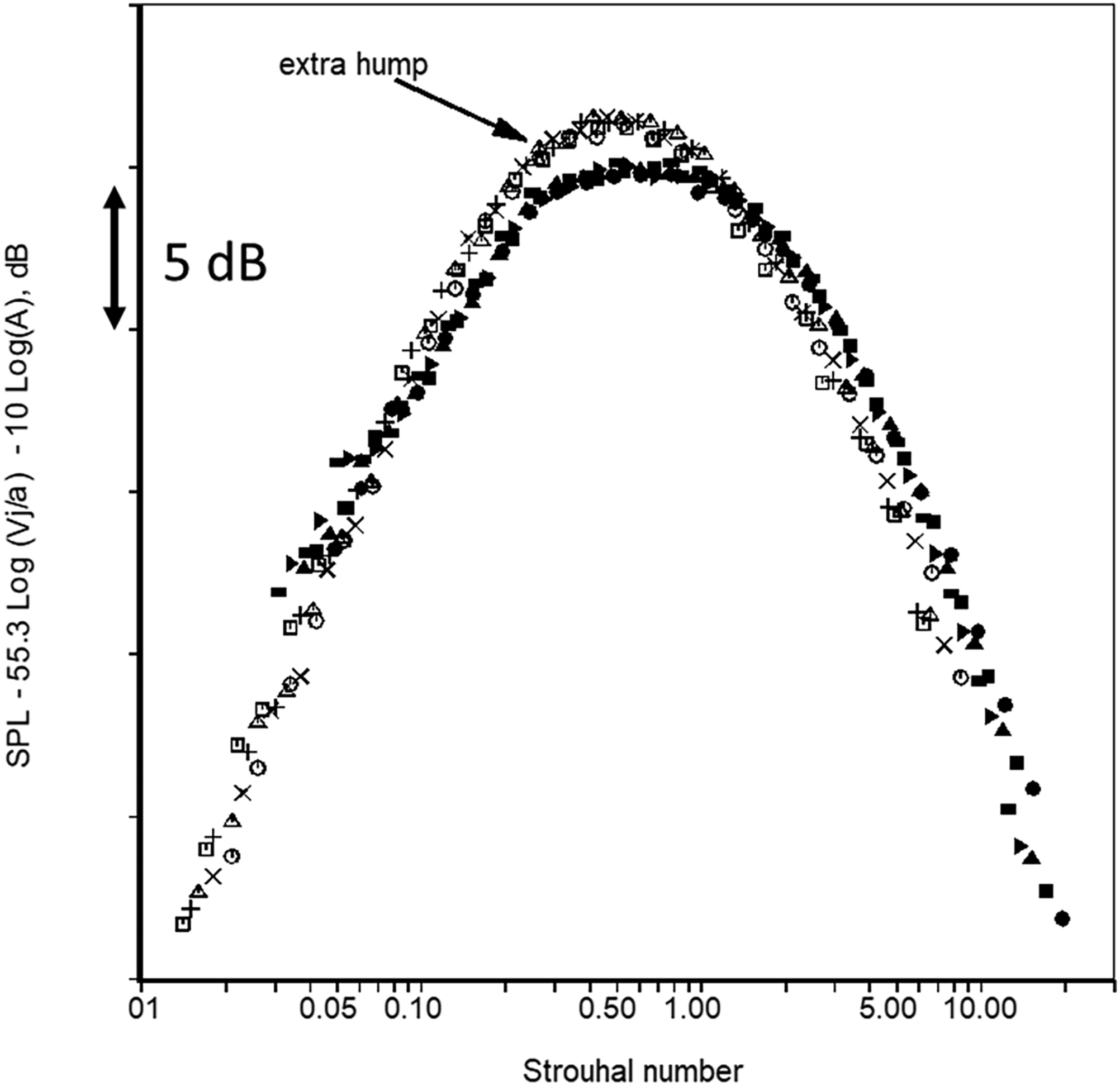

Many theoreticians of jet noise maintain that an extra source of noise of the dipole type is important at high temperatures, especially at low Mach numbers. As seen above, the dipole contribution was thought to cause the extra hump in the spectra from heated jets. In Figures 9–12 we notice the supposed presence of dipoles in the spectra obtained with the smallest nozzle (D = 1.5″) while there is no evidence of dipoles in the noise of larger nozzles. Obviously, the extra hump seen with small nozzles is due to Reynolds number effects as demonstrated in Figure 12 and has nothing to do with the presence of dipoles. It is worth reiterating the point that the Reynolds number decreases with increasing temperature, when a jet is heated at a fixed Mach number. A critical value of the Reynolds number that would need to be maintained to avoid the effects associated with low Reynolds number has been estimated to be ∼ 400,000, while a value of 500,000 or more would be desirable.

Effect of initial conditions: Laminar vs. turbulent boundary layer

Most noise tests do not include flow measurements. The large scatter in noise data acquired at various facilities is a cause for concern. Flow distortion, both in pressure and temperature, thickness and state of the boundary layer, quality of the measurement system and anechoic chamber, and analysis procedure could all play a role in the observed variations in data from different experiments. An extensive search of the literature failed to turn up any study that has systematically addressed this problem. Since the early investigation of Bradshaw,⁵⁵ there have been numerous studies on the effect of the initial conditions on the development of the flow field; see Lau,⁵⁶ Lepicovsky et al.,⁵⁷ Lepicovsky,⁵⁸ for example. A majority of these studies were restricted to extremely low Mach numbers to facilitate the use of hot wires, and were restricted to unheated jets. Given the difficulties associated with measuring clean noise at low jet velocities, the value of the conclusions for noise is dubious. Among the salient results of the various studies, two are highlighted here: (1) a strong correlation exists between nozzle exit boundary conditions and jet development, Lepicovsky⁵⁸; (2) an increased spreading rate can be achieved only in the developing region of a jet – regardless of the events in the developing region, all jets attain similar spreading characteristics far downstream, Zaman.⁵⁹

All the above studies focused on the influence of the inflow conditions on the flow development and not on the noise. A search of the literature (to the best of the author’s knowledge) revealed a few exceptions. Moore⁶⁰ examined the noise characteristics of subsonic jets with different initial conditions and determined that there was only a minor difference in noise levels. However, it is unclear if the characteristics of the boundary layers were very different since the nozzle geometries were not too dissimilar to the conic nozzle used in the current study. Zaman⁶¹ sought to quantify the effects of the initial conditions on noise for unheated subsonic jets. His results indicated that by tripping the boundary layer, one could reduce the noise levels at very low Mach numbers. Above a Mach number of 0.4, however, there was no effect due to tripping. As noted by Zaman,⁶¹ the trends for noise at very low Mach numbers and Reynolds numbers from different experiments were not consistent. Zaman⁶² carried out detailed measurements of the exit boundary layer, distributions of mean velocity and turbulence intensities, as well as the near field pressure and the far field spectra from an unheated jet at a Mach number of 0.5. Bridges and Hussain⁶³ investigated the effect of the initial condition on the sound generated by vortex pairing in unheated jets of low Mach number and confirmed that the noise produced by vortex pairing was not the dominant noise mechanism at practical jet velocities.

Here, we restrict our attention to jets at higher Mach numbers. Viswanathan and Clark⁶⁴ carried out a joint computational and experimental program to establish the effects on noise. Many references are cited in this paper and are not repeated here. It is crucial to decouple the effects on noise due to Reynolds number from those due to the state of the boundary layer. The main results from this reference are summarized here. Three nozzles of identical exit diameter (3.46 inch) have been designed and built. Based on the premise that apart from the variability in the jet rigs and nozzle construction, the state of the incoming flow to the nozzle and subsequent expansion through the nozzle is the primary candidate to have an effect on the aerodynamic performance and noise radiated, the internal contours of the nozzles were carefully shaped to control the thickness of the boundary layer. In past measurements, the Reynolds number was varied by changing the jet Mach number and certain trends were observed at low jet velocities. Then, conclusions were made as to the effects of the Reynolds number and the Mach number. However, it is not possible to isolate the effect of the state of the boundary layer from that of the Reynolds number with this approach. This ambiguity is avoided in the current study by maintaining the same Reynolds number while changing the characteristics of the boundary layer through nozzle shaping. For the results presented, the lowest Reynolds number is ∼ 577 000, which obtains for a highly heated jet with temperature ratio of 3.2 at a Mach number of 0.8. No flow field surveys have been carried out; however, the CFD results are taken to represent the prevailing flow conditions.

In-depth aerodynamic performance data presented in Viswanathan and Clark⁶⁴ indicate that the boundary layers are very different for the three nozzles and that the measured aerodynamic performance is consistent with the CFD results. Here, attention is restricted to the conic and cubic nozzles, as they have completely different boundary layer characteristics and represent the extremes. Typical gross features of the axial velocity fields for the conic and cubic nozzles are shown in Figure 13, for M = 1.0 and T_t/T_a = 2.7. Attention is drawn to the qualitative features, such as the thicker boundary layer build-up for the conic nozzle and the rapid acceleration of the flow with a very thin boundary layer for the cubic nozzle. There is also pronounced flow separation at the upstream edge of the contoured section for the cubic nozzle. The computed velocity profiles at the nozzle exit plane for the three nozzles have been examined for three Mach numbers of 0.8, 0.9 and 1.0 and two temperature ratios of 1.0 and 2.7 for each Mach number. We define the thickness of the boundary layer (δ) as the distance at which the local velocity reaches 99% of the value in the core. The boundary layer for M = 1.0 and T_t/T_a = 1.0, based on the above definition, is the thickest for the conic nozzle with a value of ∼5 mm. The long cylindrical section, which precedes the conic nozzle, serves to age the boundary layer. The cubic nozzle has the thinnest boundary layer, ∼1 mm (0.011D), with the ASME nozzle having an intermediate value of ∼3 mm.

Figure 13.

Gross features of the distribution of axial velocity. M = 1.0, T_t/T_a = 2.7. top: conic nozzle; bottom: cubic nozzle.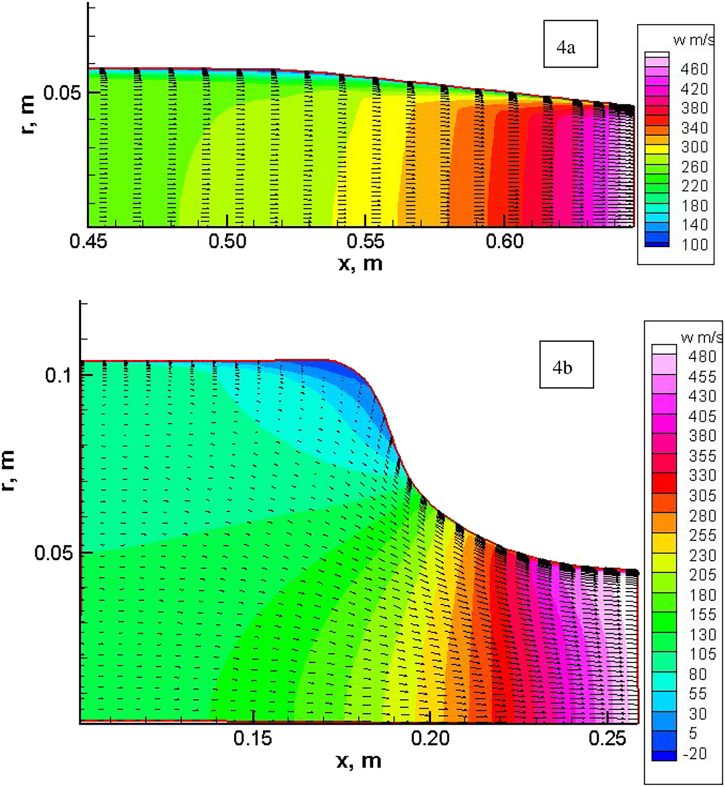

Grosche⁶⁵ investigated the sound sources in subsonic and supersonic jets through the use of an elliptical mirror. As part of this study, he examined the changes in the source distribution from initially laminar and turbulent jets. The jet diameter was 0.79″ and the Mach number of the unheated jet was 0.7. The clean nozzle was thought to produce a laminar boundary layer; a trip ring attached upstream of the nozzle exit produced a turbulent boundary layer. Figure 17 of this reference showed that the laminar boundary layer resulted in a higher noise production close to the nozzle exit than the turbulent boundary layer. This effect became more pronounced with increasing frequency, with the source levels being ∼8 dB higher for the laminar boundary layer. The increased levels were confined to a small axial distance, x/d < 2.5. Grosche⁶⁵ believed that the increased levels were caused by ring vortices or coherent structures very close to the nozzle exit. However, no spectral comparisons at the far field were presented to quantify the differences between the initially laminar and turbulent jets, though it was stated “Figure 17 demonstrates a very distinct influence of the boundary layer condition inside the nozzle upon the noise generation of subsonic jets”. Presumably, the reader is supposed to infer from this result that the jet with the initial laminar boundary layer would produce higher noise levels at the highest frequencies in the far field. It would be interesting to see if our expectations for noise, based on the current nozzle geometries and boundary layer features, are borne out by measurements.

Figure 14 shows spectral comparisons from the three nozzles from an unheated jet at a Mach number of 1.0 at three angles of 50°, 90° and 145°. For this unheated jet, a high value of Mach number is chosen to avoid the influence of the rig noise. The spectral levels for the cubic and conic nozzles are virtually identical, while the ASME nozzle generates higher levels of noise over a broad range of higher frequencies to the right of the spectral peak at the lower angles. The magnitude of the noise increase is 2⁺ dB in the forward quadrant and in the near-normal angles. As we move aft, the magnitude of the increase becomes less pronounced. Spectral comparisons are shown for a heated jet with a Mach number of 1.0 and a temperature ratio of 2.7 in Figure 15. As for the unheated jet, the ASME nozzle is the loudest, with a noise increase of ∼3 dB at the higher frequencies. The range of angles where this increase is prominent is from 50° to 100°. The spectral levels generated by the cubic nozzle are also slightly higher than those for the conic nozzle, especially at 90°. However, even at 90°, the magnitude is only ∼1 dB. In the peak radiation sector in the aft angles, the peak levels for the three nozzles are nearly identical, with the ASME nozzle generating slightly higher levels at the higher frequencies. A possible mechanism for the higher levels for the ASME nozzle is described in Viswanathan and Clark.⁶⁴

Figure 14.

Spectral comparisons. M = 1.0, T_t/T_a = 1.0. Solid: conic; dashed: cubic; dotted: ASME.

Figure 15.

Spectral comparisons. M = 1.0, T_t/T_a = 2.7. Solid: conic; dashed: cubic; dotted: ASME.

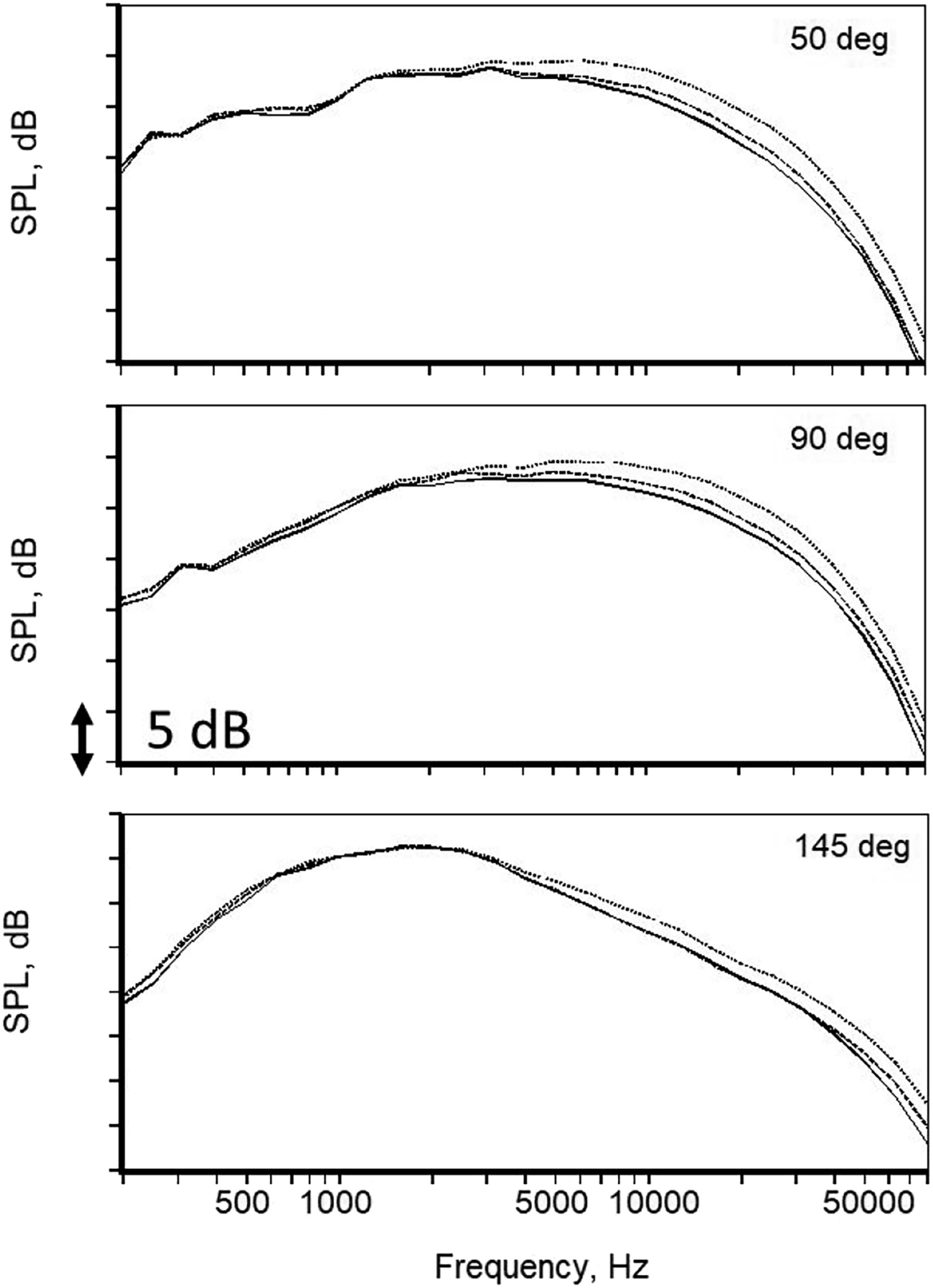
In summary, the noise levels for the conic and cubic nozzles, with thick and thin boundary layers, are nearly identical. It remains to be verified if the boundary layer is indeed laminar for the cubic nozzle. Typically, no boundary layer measurements are made in noise tests carried out in the industry. Therefore, one has to rely on CFD to investigate this issue here. This is not ideal, but there is no other recourse. The cubic nozzle was specifically designed to eliminate/minimize the upstream boundary layer buildup from the rig, with a resultant short nozzle and intense acceleration (Figure 13 bottom). One of the unknowns is whether the exit boundary layer is fully turbulent for the three nozzles. The issue of the boundary layer being laminar or transitional in most model scale experiments is well known. Jones and Launder⁶⁶ provide a detailed treatment of this problem for a generic flow (also see the references therein). There have also been several excellent review articles on this subject, see Narasimha and Sreenivasan,⁶⁷ for example. As mentioned in Jones and Launder,⁶⁶ several researchers in the 1960s discovered that the value of an acceleration parameter provided a reasonable indicator of whether turbulent boundary layers in nozzles would decay towards a laminar flow. The acceleration parameter K is defined as [ν/U² (dU/dx)], where U is the local freestream velocity and ν the kinematic viscosity of the fluid. Many characteristics of the boundary layers and their variations for different values of K were established in these experimental studies. Two salient results from Jones and Launder⁶⁶ are mentioned: (1) there is no discernible ‘universal’ logarithmic region in the velocity profile for a value of K greater than about 1.0 × 10⁻⁶; (2) above this acceleration level, the relative thickness of the viscous sublayer increases progressively with K until a value is reached at which the turbulent flow can no longer be sustained. The value of K at which relaminarization occurs was estimated to be 3.0 × 10⁻⁶. Spalart⁶⁸ carried out direct numerical simulations of sink-flow boundary layers at various values of K. The numerical simulations confirmed that relaminarization occurs at the above value of K. Several criteria and parameters have been proposed in the literature for the identification of the relaminarization process, see Brandt⁶⁹ and Mukund.⁷⁰ The difficulties with using K here are described in Viswanathan and Clark.⁶⁴ Brandt⁶⁹ proposed an alternate parameter K* defined as [K* = ν/U_o² (dU/dx)]. Here, U_o is the velocity at the location where the acceleration of the flow commences. K* introduces a history effect, whereas K is local. Brandt determined that the value for K* was greater than ∼8.0 × 10⁻⁶ for all relaminarizing flows.

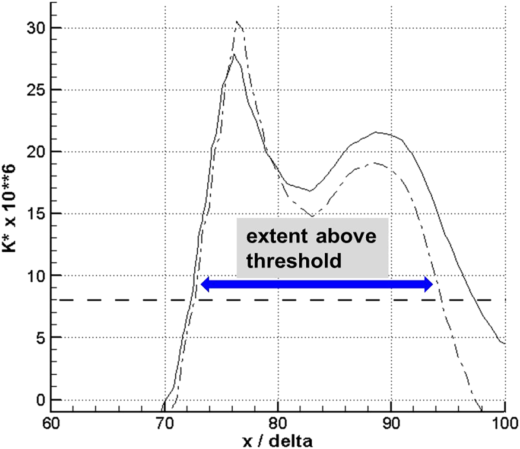
For a boundary layer on a flat plate, “x” usually coincides with the flow direction. Here, the derivative is calculated with respect to a streamline coordinate “s” [even though the notation of “x” is used]. Figure 16 shows contours of K* for the above case. It is readily seen that the picture is much clearer with this parameter (instead of K, see Viswanathan and Clark) and that there is an extended region of the flow where the values of K* exceed the threshold value. It has also been established in earlier studies that in addition to high values of the acceleration parameter, the extent of this region should be “many” boundary layer thicknesses long for laminarization to occur. We examine this feature as follows. The boundary layer thickness (δ) [and the displacement thickness (δ*)] at the nozzle exit is calculated. Next we track the value of K* along a streamline close to the edge of the boundary layer and an adjacent one. The variations of K* with (x/δ) are shown in Figure 17. Here, δ is the thickness of the boundary layer at the nozzle exit; the choice of this value bounds the problem since the thickness of the boundary layer would be smaller inside the nozzle. Typically, the distance along the streamwise coordinate is longer than x, especially close to the wall. Figure 17 indicates that there is a region of substantial length, ∼25δ, over which K* is above the threshold value. (The extent of this region would be longer if the streamwise distance s is used instead of x). There is a strong indication that the flow is laminar at the nozzle exit.

Figure 16.

Contours of the acceleration parameter K*. Cubic, M = 1.0, T_t/T_a = 2.7. U_o = 100 m/s.

Figure 17.

Variation of K* with axial distance. Cubic, M = 1.0, T_t/T_a = 2.7. U_o = 100 m/s.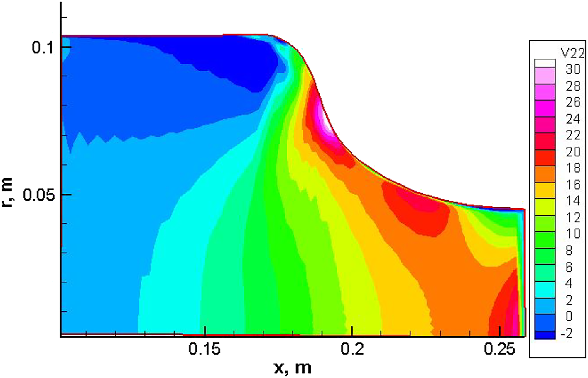

A possibly surprising conclusion is drawn from the above results. It has been determined that the state of the boundary layers is dramatically different for the short cubic and conic nozzles. Yet, the noise signatures are nearly identical. Perhaps the statement by Grosche,⁶⁵ unintended probably, caused much confusion and led to the mistaken belief that “jets with thin laminar boundary layers generate more high-frequency noise”. As demonstrated here, that is not the case at all.

The use of the acceleration parameter K* for establishing the state of the boundary layer does not provide conclusive proof, though certain insights may be gleaned. Recently, Zaman⁷¹ made boundary layer measurements from a conic and ASME nozzles; one of the variants of the ASME nozzles had a short straight section; another had an extension of a straight pipe of 3D to the end of the short section. The boundary layer characteristics were classified as turbulent, nominally laminar, and highly disturbed laminar. This study confirmed that the ASME nozzle (highly disturbed laminar) generates higher levels of noise than the conic (turbulent), as seen in Viswanathan and Clark.⁶⁴ Interestingly, the OASPL directivities from the nozzle with the extension are almost identical to those from the conic nozzle at all the Mach numbers (Figure 14); the boundary layers are classified as turbulent for both. Unfortunately, no noise measurements were taken for the short nozzle, which had a “nominally laminar” boundary layer. The author states that this short nozzle is similar to the cubic nozzle tested at Boeing. This is a real pity, as a definitive answer might have been obtained, with both noise and boundary layer data. Zaman also posits that a distinction should be made between “university-type” jet rigs and “industrial-type” jet rigs. The aeroacoustic facilities at Boing LSAF, NASA AAPL and QinetiQ NTF are classified as “industrial-type”. Viswanathan⁴² assessed the data quality from QinetiQ (and Tanna’s data) through comparison with the Boeing database and concluded that there is some extraneous contamination in the QinetiQ spectra.

In closing, this effect of the boundary layer is an interesting research question, but has little practical impact. All nozzles on engines are conical, with turbulent boundary layers. Even the divergent sections of military engines with CD nozzles have straight walls. Let us re-examine Figure 7 here; data from several conical nozzles of varying diameters and at several Mach numbers were used to produce the collapsed smooth spectral shape. Obviously, the only way to assure clear-cut and unambiguous spectral quality is through scaling at all angles and all frequencies, for both unheated and heated jets. It should be incumbent on experimentalists using any facility to first provide this proof, before analyzing and reporting trends. This approach is simple, straightforward and obviates the need for complicated boundary layer measurements. The supposition that a “university-type” rig would generate higher levels of noise is not based on concrete evidence, unless the quality is first established beyond doubt.

Effect of temperature on jet noise

A systematic study has been undertaken to quantify the effect of jet temperature on the noise radiated by subsonic and supersonic jets. Again, several nozzles were utilized. The test matrix consisted of three series: for one set of data, the Mach number of the jet [or nozzle pressure ratio (NPR)] was held constant and the jet stagnation temperature was increased progressively. For the second set, data were acquired at constant jet velocities obtained through the proper choice of NPR and temperature ratio, in order to quantify the so-called “density effect”. For the third set, the jet static temperature ratios were held constant and the Mach number was varied. Typically, aeroacoustic data have been obtained at seven stagnation temperature ratios (T_t/T_a) of 1.0, 1.8, 2.2, 2.7, 3.14, 3.2 and 3.51 for the first set. Only three static jet temperature ratios (T_j/T_a) of 2.0, 2.5 and 3.0 have been considered for the third set, because it is complicated and time-consuming to generate data at fixed static temperature ratios. Attention is drawn to the fact that the stagnation temperature ratio of 3.2 is higher than the operating cycle conditions of all turbofan engines in service. The highest ratio of 3.51 was later added to simulate the temperature of a military jet engine. An extensive database has been generated to answer many fundamental questions on the noise of hot jets as well as to provide high-quality data for the development of prediction methods for jet noise. The salient results from Viswanathan^48,72–74 are highlighted here.

Effect of temperature on power level and overall sound pressure level

The eighth-power dependence of the OAPWL on jet velocity was established circa 1950. Here, the power levels and overall sound pressure levels have been computed per unit nozzle area, through the subtraction of [10*Log₁₀(A)]. The variation of OAPWL with acoustic Mach number is shown in Figure 18. Also shown is a line representing a V⁸ variation. At first look, all the points seem to follow the eighth power law. Let us take a closer look and isolate the temperature effect by grouping the points as per the temperature ratio. Figure 19 shows the same plot, with the curves spaced apart, and a least-square fit through each group. As can be seen, the value of the velocity exponent decreases with increasing temperature, from a value of 8.74 for unheated jets to a value of 7.98 for heated jets at a temperature ratio of 3.2. Note that the value of the exponent is close to eight for the highly heated cases. It is evident that at no jet temperature is a V⁶ dependence observed. In Figure 18, two other values at Mach numbers of 0.3 and 0.4 (unheated) were included, denoted by the open squares. At these low Mach numbers, rig noise becomes an issue and the value of the velocity exponent obtained with these two values included with the other six, yields a value of 8.41 (down from 8.74) for the unheated cases. It is clear that contamination by rig noise, which is a big factor at low Mach numbers, could influence the value of the velocity exponent as shown in the above example.

Figure 18.

Variation of OAPWL with jet velocity, D = 2.45”. Solid line: V⁸. □,■: T_t/T_a = 1.0; x: T_t/T_a = 1.8; Δ: T_t/T_a = 2.2; o: T_t/T_a = 2.7; •: T_t/T_a = 3.2.

Figure 19.

Variation of OAPWL with jet velocity, D = 2.45”. ■: T_t/T_a = 1.0; x: T_t/T_a = 1.8; Δ: T_t/T_a = 2.2; o: T_t/T_a = 2.7; •: T_t/T_a = 3.2.

This subtle dependence of OAPWL on jet temperature was detected and reported first by Viswanathan,⁴⁸ nearly 50 years after the eighth-power dependence was determined. Following this idea of isolating the effect of temperature, variations of the overall sound pressure level (OASPL) and spectra were subsequently investigated. But first, we re-plot the OAPWL variation (from Figure 18) using a linear axis for the acoustic Mach number on the x-axis to glean some insights; see Figure 20. Least-square curve fits for the two extreme temperature cases, T_t/T_a = 1.0 and 3.2, are also shown. The slopes of these two curves suggest that at an acoustic Mach number of ∼0.8, the two curves could intersect. Also, this figure suggests that there is a small velocity range in which the power radiated by jets at different temperatures would be more or less the same. Hoch et al.⁷⁵ and Tanna et al.⁵⁰ quoted a value of 0.73 from their measurements. However, as seen in Figure 20, pinpointing a single value would be very difficult. Furthermore, the trends allow for the possibility that at lower relative velocities, a heated jet could produce more noise than a cold jet at fixed velocity, while the reverse is true in the higher velocity range.

Figure 20.

Variation of OAPWL with jet velocity, D = 2.45”. ■: T_t/T_a = 1.0; x: T_t/T_a = 1.8; Δ: T_t/T_a = 2.2; o: T_t/T_a = 2.7; •: T_t/T_a = 3.2.

The variation of OASPL of the radiated noise at 90°, where the contribution of the noise from large-scale structures is negligible, as a function of the acoustic Mach number is shown in Figure 21 (top). Again, the test points are grouped as per temperature ratio. Least-square curve fits are shown for two cases, with T_t/T_a = 1.0 and 3.2. The slopes of the curves (velocity exponents in this direction) decrease continuously as the jet temperature increases: from a value of ∼8 for the unheated case to 5.53 for T_t/T_a = 3.2. These trends are very similar to the ones observed for the overall power level, with the possibility that the hotter jets could radiate more noise in this direction at lower velocities. A similar variation of the intensities at 160° is shown in Figure 21 (bottom). As at 90°, there is a family of curves with decreasing slopes. The value of the velocity exponent again decreases as the jet temperature increases, from a value of 9.67 for the unheated case to 7.67 for T_t/T_a = 3.2.

Figure 21.

Variation of OASPL with jet velocity, D = 2.45”. Top: 90°, bottom: 160°. □: Tt/T_a = 1.0; o: T_t/T_a = 1.8; Δ: T_t/T_a = 2.2; x: T_t/T_a = 2.7; •: T_t/T_a = 3.2.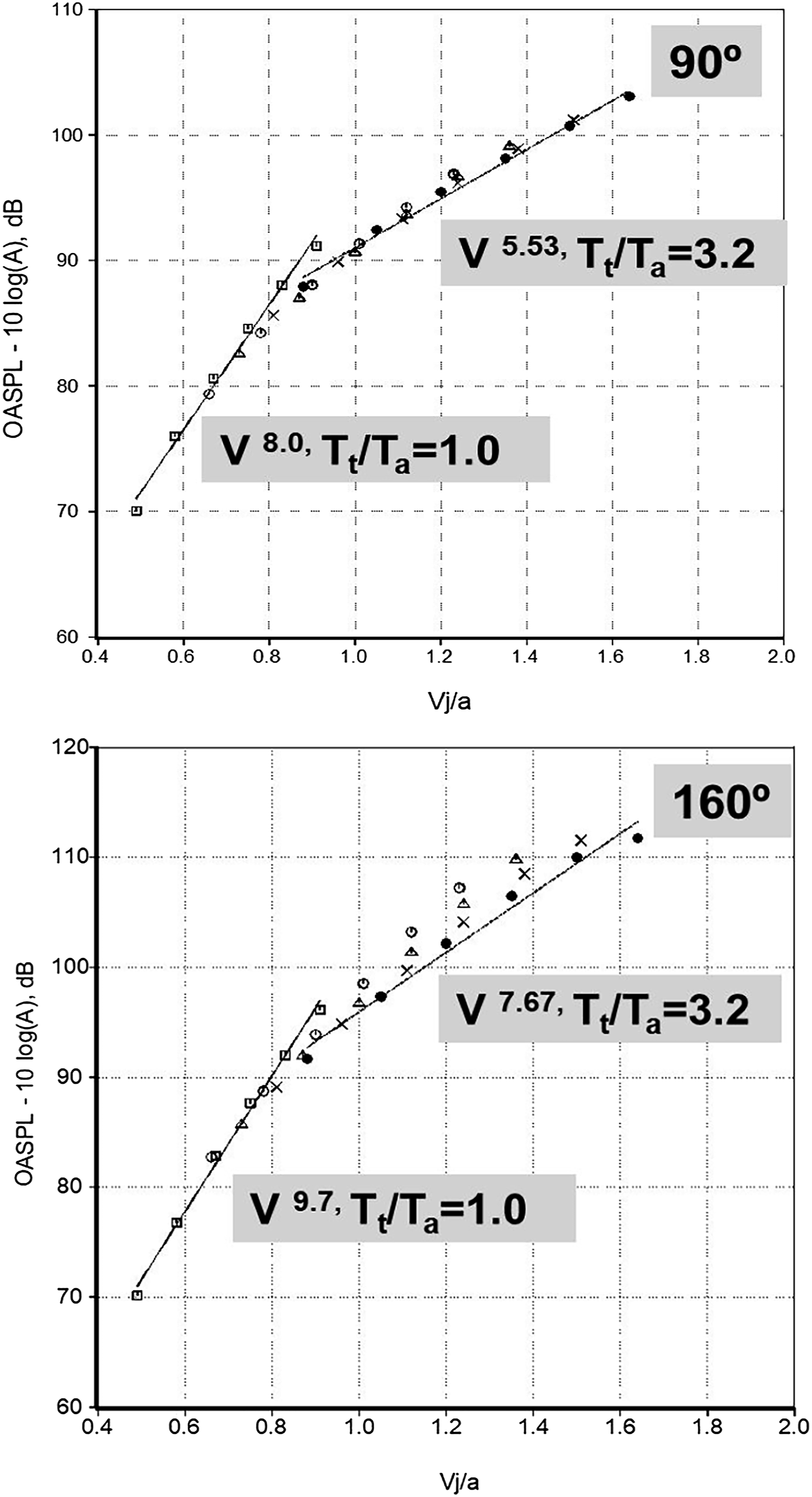

The velocity exponents have been calculated from the database, both for fixed stagnation and static temperature ratios at all polar angles. Figure 22 shows these variations with angle; first of all, the trends are very similar for the heated jets. In the forward quadrant and up to ∼90°, the curves are generally flat, with only a small increase in value. When we move to the aft quadrant, there is a rapid increase, with the highest values in the peak radiation direction. The highest values are seen for the unheated jet; the value of the exponent is ∼ 8 at lower angles and reaches ∼9.7 at aft angles. There is a sharp decrease in levels with increasing temperature ratios at the lower angles. Thus, there is a pronounced effect of jet temperature on the OASPL. Attention is drawn to the fact that there is only a weak dependence of OASPL on temperature in the peak radiation sector, unlike at the lower angles. These high levels at aft angles would contribute the most energy in the calculation of OAPWL. Perhaps this weak dependence of OASPL explains the weak dependence of OAPWL on temperature, as seen in Figure 19. Before we examine the spectral variations, results for the density effect on sound power are presented.

Figure 22.

Velocity exponent for various angles. Fixed jet total and static temperature ratios.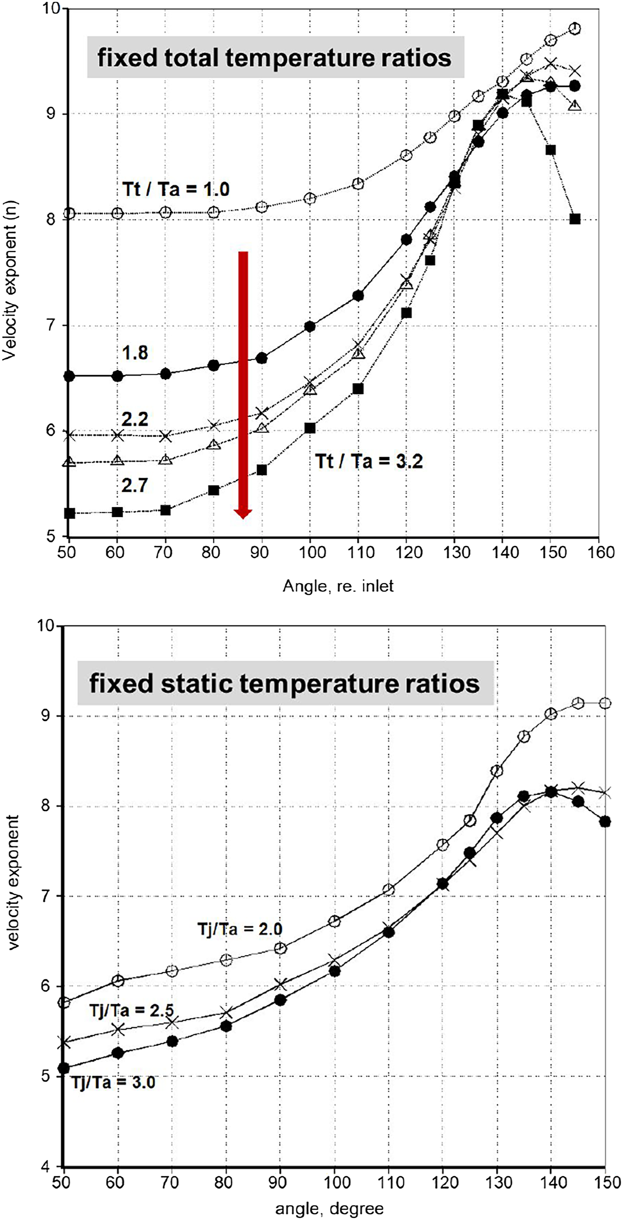

Noise of jets at fixed jet velocities: The density effect

First, the propulsive issues with studying jets at fixed jet velocities must be considered. With a suitable combination of NPR and temperature, one could attain a desired jet velocity. A thorough treatment of the nozzle aerodynamic characteristics is described in Section 3 of Viswanathan.⁴⁸ The measured thrust is only a function of NPR. The jet total temperature has an indirect effect since the gas constant (γ) is a function of temperature. When the jet is heated, the value of γ typically decreases. For the propane fuel used to heat the jet in the above experiments, the value of γ for the fuel/air mixture decreases from 1.4 at ambient temperature to approximately 1.34 at 944 K. This results in a decrease in thrust of ≈0.5% at a fixed NPR. Thus, the jet temperature has a weak effect on thrust. A crucial point should be kept in mind when examining the effect of jet temperature on noise at fixed jet velocity. Clearly, the thrust level decreases as the nozzle pressure ratio is decreased and the temperature is increased to produce the same jet velocity. Consequently, comparisons of noise at fixed jet velocity are not made at constant thrust.

In order to quantify the effects of density variation, measurements were taken at six values of (V_j/a) of 0.53, 0.62, 0.73, 0.8, 0.9 and 1.2. The corresponding jet velocities are 600 ft/s (183 m/s), 700 ft/s (213 m/s), 820 ft/s (250 m/s), 900 ft/s (274 m/s), 1010 ft/s (308 m/s) and 1350 ft/s (412 m/s), respectively. Since convergent nozzles have been used, data have been acquired only at heated conditions for the highest velocity case (V_j/a = 1.2) to avoid shock noise. Eight reservoir temperatures, ranging from T_t/T_a = 1.0 to 3.05 have been considered at each velocity, for this particular study. The utmost care is necessary, and has been exercised, in acquiring data at the lower velocities so as to avoid the Reynolds number effects and corruption by rig noise. As noted already, a Reynolds number of ∼400,000 would be adequate, while a value of 500,000 or more would be desirable. However, the transition spans a range of Reynolds numbers from ∼300,000 to ∼350,000. In the following figures, even though data were acquired at all eight combinations of NPR and temperature ratio at a particular jet velocity, only the test points that produced a Reynolds number of at least 335,000 have been included. Thus, any ambiguity with the results that may be attributed to the effects of Reynolds number is eliminated.

The overall power levels at each velocity for several jet temperatures are shown in Figure 23. The velocities have been chosen carefully such that two of them are in the transition region where the power levels remain more or less constant, while there are two values each at higher and lower velocities. As seen in other measurements, the radiated power decreases with increasing temperature in the high velocity regime (Figure 23(e) and (f)). While the reduction is more pronounced at V_j/a = 1.2, the value is more modest at V_j/a = 0.9. Examination of Figure 20 indicates that the noise picture is not clear-cut at V_j/a = 0.9. In the transition region, at velocities of 0.73 and 0.80 (Figure 23(c) and (d)), the power level remains more or less constant for different jet temperatures. In the lower velocity regime (Figure 23(a) and (b)) the trends are reversed, with the noise power increasing with increasing jet temperature. There were some questions about the older measurements at the lower velocities, which the current data has helped clarify. Hence, it is evident that the effect of jet temperature on the radiated noise is very different at different fixed velocity regimes.

Figure 23.

Variation of OAPWL with jet temperature. (a) Vj/a = 0.53; (b) 0.62; (c) 0.73; (d) 0.80; (e) 0.90; (f) 1.2.

Scaling of spectra

The scaling of spectra has practical application, as it forms the foundation for empirical predictions. There have been several attempts in the past to collapse spectra from heated and unheated jets; most of these have relied on acoustic analogy, together with other theoretical considerations. In many of these, scaling laws for jet noise were developed for a radiation angle of 90°, where convection and other effects are negligible. A review of all the classical formulations is provided in Section III.B of Viswanathan.⁷² The general form of the different formulations may be represented by,

I_{90} \propto A_{1} {(\frac{V_{j}}{a})}^{8} + B {(\frac{V_{j}}{a})}^{6} + C {(\frac{V_{j}}{a})}^{4}

(2)

A₁, B, and C are complicated functions of the jet static temperature and the functional forms depended on the assumptions invoked, with several empirical factors introduced. Fisher et al.⁴⁹ assumed that the Reynolds stress term and the entropy term are independent and uncorrelated, and came up with the second source producing a V⁴ dependence. The model of Lilley⁸ consisted of all three source terms; the model of Tanna et al.⁵⁰ favored only the quadrupole and monopole terms, with the velocity exponent for the quadrupole term being 7.5 rather than 8.0. When Tanna et al.⁵⁰ tested their formulation against data from hot jets, they were forced to make a further assumption that the two sources must be correlated. Morfey et al.⁵³ developed scaling laws based on geometric acoustics and examined the importance of the three assumed sources of monopole (V⁴), dipole (V⁶), and quadrupole (V⁸), and their contributions to the total noise, with and without these sources being coherent. They concluded that the combination of dipole and quadrupole sources with zero coherence best represented the data. In the model of Fisher et al.,⁴⁹ it was suggested that the contribution from the quadrupole term decreased with increasing jet temperature. Morfey⁷⁶ reasoned that this term should be independent of temperature. His model also predicted that at higher V_j/a, the noise from heated jets at lower frequencies should be independent of jet temperature, while the spectral levels at higher frequencies would diminish as (T_j/T_a)^−3.5. Goldstein⁷⁷ derived a variant of the Lilley’s equation without introducing additional approximations and represented the sources as the sum of quadrupole and dipole terms. Goldstein⁷⁷ derived a different set of linearized inhomogeneous Euler equations that produced quadrupoles and monopoles as the source terms. It is clear then that there are no commonly accepted sources of jet noise even among well-established researchers, with different researchers invoking disparate theoretical arguments (and associated assumptions) to support their formulations. Not surprisingly, none of these formulations yielded good spectral collapse even at 90°.

The situation becomes more complicated at aft angles. In Lighthill’s acoustic analogy, the equivalent sources move but the medium is at rest. It is well established that sources in motion radiate more noise in the direction of motion. As the jet velocity increases, the effect of source convection becomes more pronounced; this problem was examined in detail by Ffowcs-Williams.⁶ The main results, following Fisher et al.⁴⁹ and taken from this paper may be summarized by the following relations:

I (r, θ) \approx \frac{ρ_{s}^{2} V_{j}^{8} D^{2}}{ρ a^{5} r^{2}} D (θ) {[1 - M_{c} \cos θ]}^{- 5}

(3)

I (r, θ, f) \approx \frac{ρ_{s}^{2} V_{j}^{8} D^{2}}{ρ a^{5} r^{2}} D (θ) {[1 - M_{c} \cos θ]}^{- 5} F [\frac{f D}{V_{j}} (1 - M_{c} \cos θ)]

(4)

In the above equations, ρ_s is the source density, and ρ is the ambient density. D(θ) is the directivity factor, with θ measured from the jet exhaust axis; M_c is the convection Mach number usually assumed to be ∼65% to 70% of the acoustic Mach number (V_j/a). In some studies, a modified Doppler shift instead of the simple Doppler shift for the frequency has been proposed:

f_{m} = f {[{(1 - M_{c} \cos θ)}^{2} + α^{2} M_{c}^{2}]}^{1 / 2}

(5)

α is an empirical constant with a value of ∼0.3. At 90°, equation (3) predicts that the intensity or OASPL varies as the eighth power of jet velocity. In the aft directions, there is a faster increase of noise with (V_j/a) due to the convective amplification factor. Equation (4) for the spectra includes a spectrum function F, which is a function of the Doppler shifted frequency. At 90°, which is perpendicular to the direction of the source convection, the observer and source frequencies are the same; the shape of the source spectrum F corresponds to the convected source spectrum. In the aft directions, the effect of source convection results in a Doppler shift of the source frequency f_s to yield an observer frequency f given by,

f = \frac{f_{s}}{(1 - M_{c} \cos θ)}

(6)

Therefore, the spectrum function F in equation (4) has a dependence on the Doppler shifted Strouhal number. The spectra in the aft angles incorporate both the effects of convective amplification and a Doppler shift of the frequency. This relation has a more complicated form when the modified Doppler shift, the effect of source non-compactness, etc. are included.

A summary of the many approaches adopted by various researchers to collapse spectra at aft angles is given in Section 4.4 of Viswanathan.⁴² Morris and Viswanathan⁴³ provide a more detailed treatment of the various classical theories. One main observation, in both the formalisms of Lighthill and Lilley, is that there is a Doppler shift for the frequency, based primarily on the notion of moving sources. It was noted even in the early 1970s that the predicted spectra in the aft angles differed drastically from the measured data; see Lush⁷⁸ and Fisher et al.⁴⁹ for example. In an effort to establish the correct velocity dependence Tanna,⁵¹ among many others, attempted different powers of the directivity factor, a downstream location for the noise source, different assumed values for M_c and α, etc. However, none of these approaches, with any combination of M_c, α and the value for the directivity exponent (−3 to −9 instead of −5) provided satisfactory results for the OASPL directivity or the collapse of the entire spectra.

A crucial omission in all of the above formulations is the lack of recognition that the jet temperature could play a fundamental role in controlling spectral shape and spectral collapse. In all fairness, this trend was discovered only ∼30 years later. As already shown, the OAPWL has a weak dependence and the OASPL has a strong dependence on the temperature ratio. Viswanathan,^48,72 and⁷³ proposed a new scaling law that explicitly accounts for the temperature ratio. The new scaling law for the spectra at any angle is given by:

S P L (θ, S t) = F (θ, S t, \frac{T_{t} o r T_{j}}{T_{a}}) {[\frac{V_{j}}{a}]}^{n}, n = n (θ, \frac{T_{t} o r T_{j}}{T_{a}})

(7)

The sound pressure level (SPL) per unit area (or area-normalized SPL) at an arbitrary fixed distance is given by the product of a spectrum function and the velocity ratio raised to the velocity exponent n. The spectrum function F and exponent n, at a particular angle and temperature ratio, are obtained from experimental measurements. When the parameter [SPL -10*Log₁₀ (A/A_ref) – 10*n*Log₁₀ (V_j/a)] for one-third octave spectra or [SPL -10*Log₁₀ (A/A_ref) - 10*n*Log₁₀ (V_j/a) - 10*Log₁₀ (D/V_j)] for narrowband spectra with constant bandwidth are plotted against the Strouhal number, a master spectral shape results for every angle and every temperature ratio. A is the nozzle exit area and A_ref is a reference area, which is taken to be one square inch here for convenience. This is the above spectrum function F(θ, St, T_{t, j}/T_a). The velocity exponent n has a unique value, and is calculated from the measured overall sound pressure levels at each angle, from jets of different (V_j/a) but with fixed jet temperature ratio, as shown in Figure 22. Attention is drawn to the following features: (1) the velocity exponent depends on either the jet stagnation or static temperature ratio; (2) there are no multiplicative functions that are dependent on temperature. As such, no adjustable empirical constants or other assumptions are needed; (3) there is no convective amplification factor in the current formulation; (4) the plain Strouhal number, without any Doppler shift, appears in the spectrum function F; and (5) the spectrum function F has explicit temperature dependence.

Sample spectral collapse at several angles are shown to highlight the efficacy of the new scaling law. Figure 24 shows normalized spectra from six different Mach numbers of 0.4, 0.5, 0.6, 0.7, 0.8, and 0.9 at an angle of 90°, for a fixed static temperature ratio of 2.0. The value of the velocity exponent is 6.42. Figure 25 shows normalized spectra from five different Mach numbers of 0.6, 0.7, 0.8, 0.9, and 1.0 at an angle of 120°, for a fixed stagnation temperature ratio of 3.2. The value of the velocity exponent is 7.46. There is a very good collapse of the entire spectrum with Strouhal number, in both cases. Of course, the span of Strouhal number for each jet velocity has a different range (raw frequency range of 200–80,000 Hz), but there is excellent overlap and a smooth master shape emerges. It is essential to use the correct velocity exponent for a particular angle and a particular temperature ratio. Attention is drawn to the fact that unlike past approaches where a “high frequency” dependence and “low frequency” dependence (though no one has defined “high” and “low” ranges for the Strouhal number) are utilized to scale different parts of the spectra, a single exponent is adequate for the collapse at all Strouhal numbers (frequencies). Furthermore, the values of the exponents have been extracted from a deep analysis of the database, without invoking any questionable assumptions, or doubtful theoretical considerations.

Figure 24.

Normalized spectra at 90° for a range of Mach numbers. n = 6.42. Fixed static temperature ratio of 2.0.

Figure 25.

Normalized spectra at 120° for a range of Mach numbers. n = 7.46. Fixed stagnation temperature ratio of 3.2.

Now we move to large aft angles. Figure 26 depicts normalized spectra at 135° at two stagnation temperature ratios of 2.2 and 3.2; Figure 27 shows normalized spectra at 145° at three stagnation temperature ratios of 1.0, 1.8 and 3.2. Note that the plain Strouhal number is used on the x-axis. There is good spectral collapse at both angles. The red arrow in Figure 26 indicates the Strouhal number for the spectral peak. Application of any Doppler frequency shift, simple or more elaborate as proposed in the past, would progressively pull the spectra left (or right) as the Mach number is increased and would destroy the spectral collapse. It is readily evident that there are two and three distinct families of curves, each with a unique shape, for all jet velocities within that temperature group. The spectral width becomes narrow as the temperature ratio increases. These figures indicate that the spectral shape at a particular aft angle is controlled more by the temperature ratio than the velocity ratio. This point is reinforced in Figure 28, which shows the spectra at eight different temperature ratios but at a fixed V_j/a = 0.8; the radiation angle is 155°. The spectra have the same shape in the low frequency regime, to the left of the spectral peak. However, at the higher frequencies, there is a progressive narrowing of the spectral width with increasing temperature.

Figure 26.

Normalized spectra at 135° for a range of Mach numbers. Fixed stagnation temperature ratio of 2.2 and 3.2.

Figure 27.

Normalized spectra at 145° for a range of Mach numbers. Fixed stagnation temperature ratio of 1.0, 1.8 and 3.2.

Figure 28.

Spectra at 155° with fixed jet velocity and eight stagnation temperature ratios.

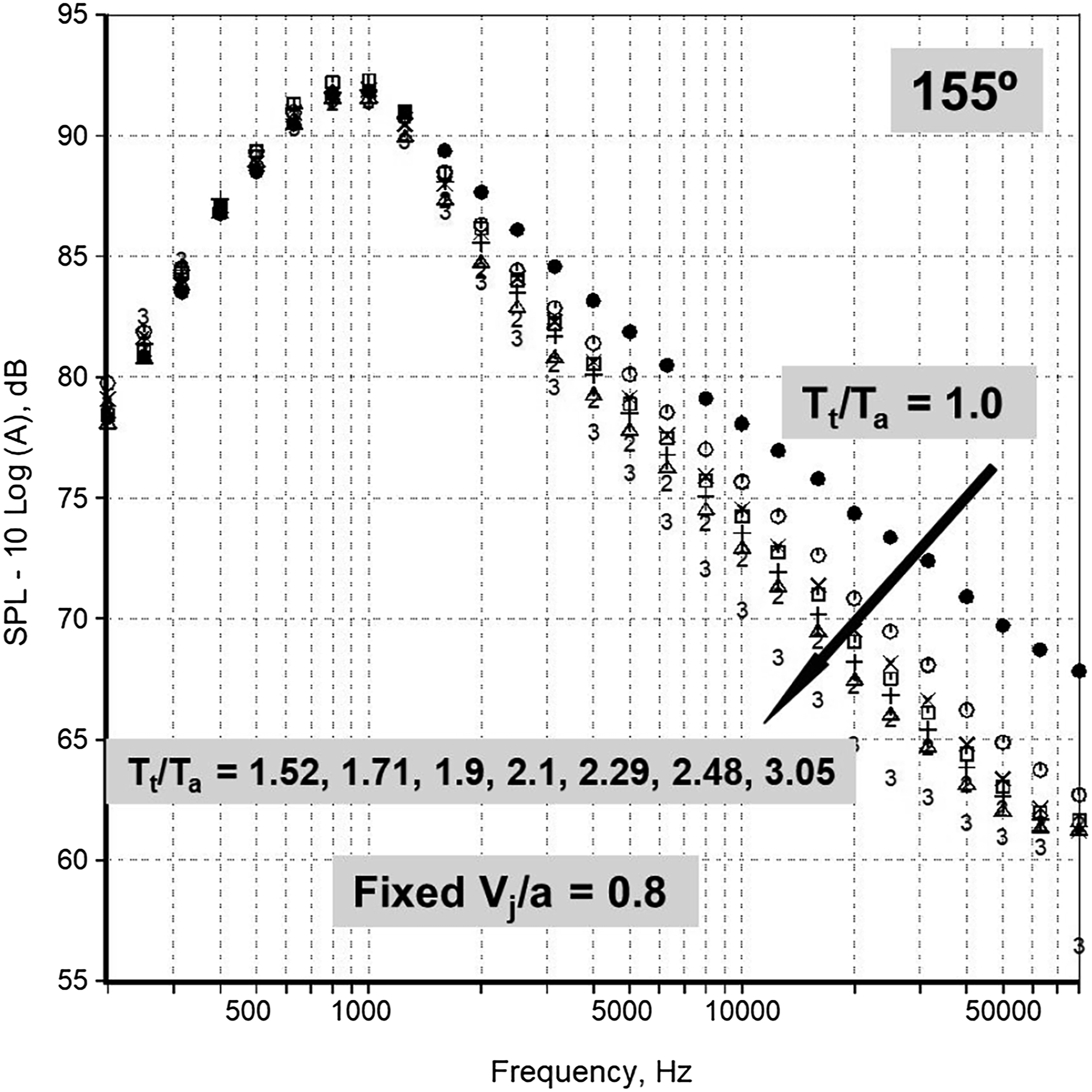
Now, let us examine the spectral shapes at large aft angles in Figures 26–28. They all have sharp peaks and rapid roll-offs away from the peaks. These characteristics were identified by Tam et al.³⁶ for the LSS shape. As seen here, there is no one unique shape for the LSS spectrum, because of the temperature effect on spectral width. This point was first broached in an earlier Section on the two similarity components.

In summary, the spectral shape at every radiation angle is controlled by the jet temperature. A single, correct velocity exponent that is a function of the angle and temperature ratio, is adequate to collapse the spectra over the entire raw frequency range of 200 Hz to 80,000 Hz, for all jet velocities at a fixed temperature. The plain Strouhal number is employed at all angles. In classical theories, [see equation (3) above, for example] terms for source directivity rely on some form of the convective Mach number M_c, which is a function of jet velocity alone. As seen here, the jet temperature controls the spectral shape in the aft angles. It is also clear now why the directivity factors based on velocity alone fail to predict the observed trends. There is also no experimental evidence for convective amplification. Based on the evidence presented here and in Viswanathan^42,72 of excellent collapse of the spectra over the entire frequency range at all the angles, we can conclude that the temperature ratio as well as the velocity ratio are indeed the two independent parameters that control jet noise.

The effectiveness of the new scaling laws is obvious from the samples shown here and from numerous cases presented in Viswanathan,^72,73,79; this is entirely due to the explicit recognition of the jet temperature ratio as an independent parameter. There is no summation of contributions from quadrupoles, dipoles and monopoles. The approach of modeling the multiplicative factors for these terms on temperature is now seen to be erroneous. When we consider the facts that, (1) the experimental data used to justify the classical theories are not accurate as shown recently, and (2) none of the theories explain or predict the experimentally observed spectral characteristics, it becomes apparent that the classical ideas of multi-pole sources for jet noise become untenable.

New prediction method

It is unambiguously established that the temperature ratio, along with the velocity ratio, is an independent and intrinsic parameter that uniquely controls jet noise. The value of the scaling law [Equation (7)] is immediately obvious, as it can be directly used for accurate spectral predictions. Curve-fits for the spectrum functions at all angles and at five stagnation temperatures of 1.0, 1.8, 2.2, 2.7 and 3.2 have been determined. A sample curve-fit is shown in Figure 29 at an angle of 110°. The shape of the curve with Strouhal number is invariant: it does not slide left or right, but moves up for a desired nozzle area and jet velocity. A prediction involves just the addition of [10*Log₁₀ (A/A_ref) + 10*n*Log₁₀ (V_j/a)] to the spectrum function at each angle, with the appropriate value for the velocity exponent. Predictions at other temperature ratios are obtained through interpolation. The author would like to acknowledge and thank his colleague Dr. Alkislar for generating these curve-fits. There is also another, perhaps under-appreciated, use for equation (7): it can be readily applied to check the spectral quality of data obtained in any facility and pinpoint the magnitude of contamination and affected frequencies.

Figure 29.

Curve-fit for spectrum function at 110°. Fixed stagnation temperature ratio of 2.7.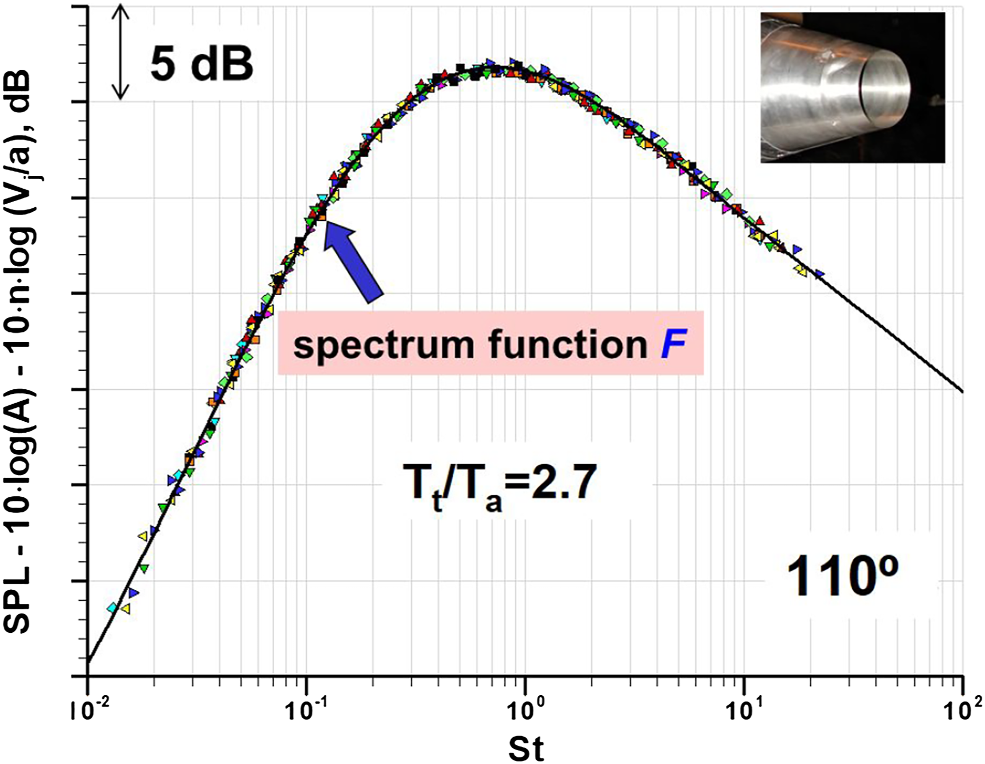

Nonlinear propagation

Detailed spectral analysis of the entire database revealed a thus-far unreported surprising effect: the manifestation of nonlinear propagation for subsonic heated jets in the peak noise radiation sector. Nonlinear propagation is usually associated with high-intensity noise events such as blast waves, shock waves, sonic booms and jet noise from military jets, especially at after-burner conditions. Figures 30 and 31 illustrate this phenomenon; the stagnation temperature ratios are 3.2 and 3.51, respectively. The radiation angles are 145° and 120°, respectively. The convective Mach number is generally assumed to be 0.7 times (V_j/a). Whereas the normalized spectra collapse at the higher frequencies for the jets with subsonic convective Mach numbers, the spectra start tailing up when the convective Mach number becomes supersonic. This fact has been verified for all supersonic convective Mach numbers. In practical terms, when the jet velocity exceeds a value of ∼1600 ft/sec, nonlinear propagation is triggered, as first reported by Viswanathan.⁷⁹ Compare Figures 27 and 30: spectra only at subsonic convective Mach numbers are included in Figure 27. It was also verified that for jets in forward flight, the relative velocity between the jet velocity and forward flight velocity (V_j - V_f) should exceed this threshold value for the onset of nonlinear propagation. Figure 32 from Viswanathan, Alkislar and Czech⁸⁰ show spectral comparisons for a shock-containing supersonic jet with M = 1.72 and T_t/T_a = 2.7, obtained with microphones from a 15-ft sideline array and a 25-ft polar array, and corrected to a common distance. Clearly, the levels at the higher frequencies are elevated for the spectra at 90°, where shock-associated noise is dominant. This study revealed that the convective Mach number is not a good indicator for the onset of nonlinear propagation for shock noise; the physical phenomenon for this manifestation is as yet not known. In the determination of the spectrum function curve-fits, care was taken not to include spectra from supersonically convective Mach numbers at the higher temperatures.

Figure 30.

Normalized spectra at 145° for a range of Mach numbers. Fixed stagnation temperature ratio of 3.2. Jet with supersonic convective Mach number included.

Figure 31.

Normalized spectra at 120° for a range of Mach numbers. Fixed stagnation temperature ratio of 3.51. Jets with supersonic convective Mach number included.

Figure 32.

Normalized spectra at 90° and 130°. M = 1.72, T_t/T_a = 2.7. Black: microphone at 15 ft; red: microphone at 25 ft.

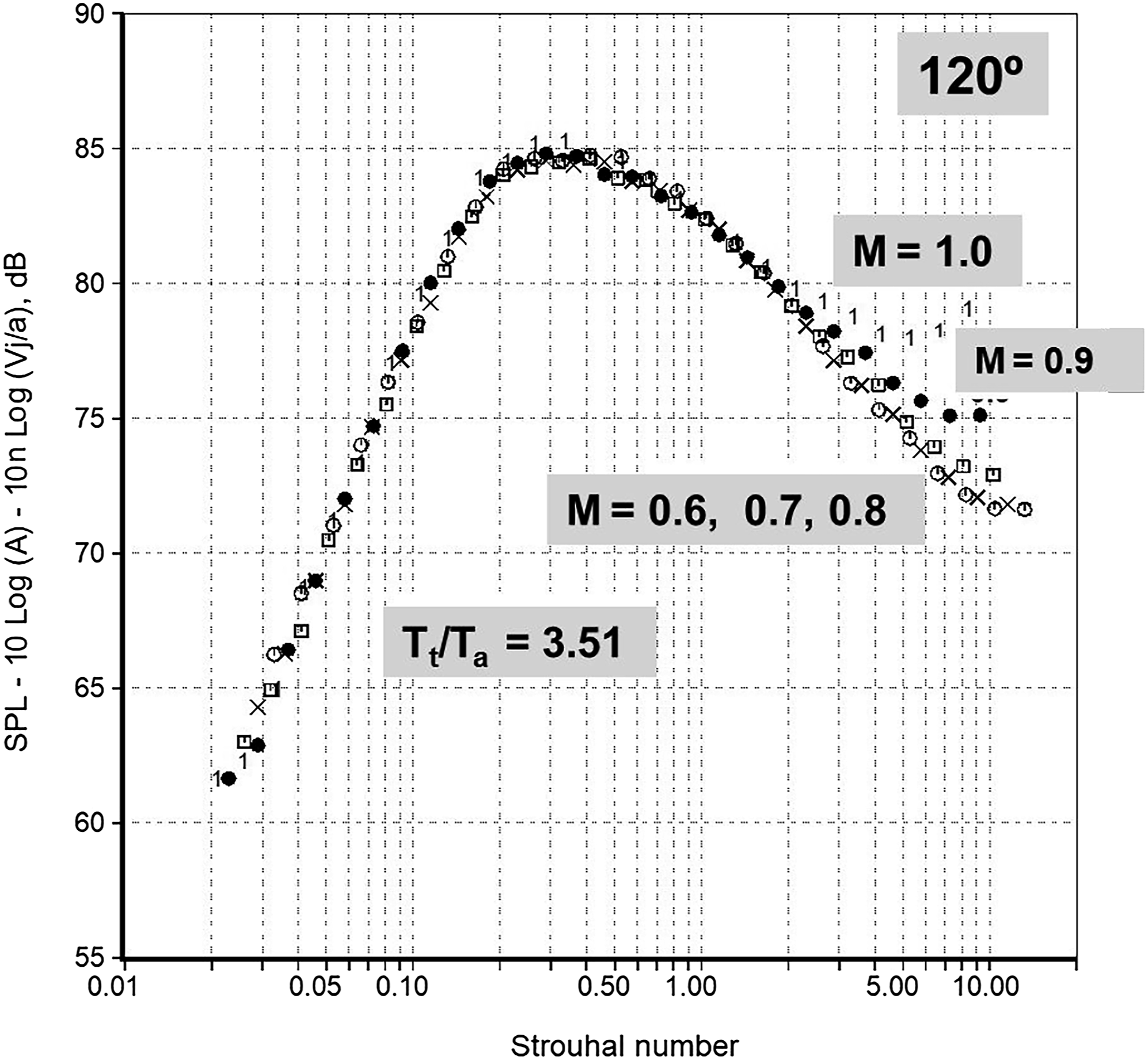
To better understand the features associated with the nonlinear distortion of acoustic waves, special experiments were conducted in LSAF, both with a convergent nozzle and a convergent-divergent nozzle with a design Mach number of 1.92. Four microphones were deployed at an angle of 150°. The non-dimensional distances (r/D) were 52, 81, 111, 150 for the convergent nozzle; the values were 100, 157, 213 and 289 for the smaller convergent-divergent nozzle. Data obtained in a controlled environment in an anechoic chamber avoids the numerous problems associated with outdoor measurements, and probably unknowable ground effects. This clean set of data is ideal for algorithm development. Time-series data and spectra were generated for a wide range of convective Mach numbers, from low subsonic to highly supersonic. A collaborative project was carried out with Professor Phil Morris and Professor Dennis McLaughlin, along with their (then) graduate students Swati Saxena and Benoit Petitjean, respectively, in the creation of a new computational method and analysis of the data. Two publications from this joint effort resulted: Petitjean, Viswanathan and McLaughlin⁸¹ and Saxena, Morris and Viswanathan.⁸² Both spectral and time-domain analyses have been performed to elucidate nonlinear effects.

The spectral analysis indicates that there is agglomeration of energy at the higher frequencies as the propagation distance increases. In the new algorithm, the generalized nonlinear Burgers equation, which includes atmospheric absorption and dissipation, is solved for the pressure signal in the frequency domain. The results are then obtained as a function of time. The experimental and predicted power spectral density plots are compared for microphones at different radial locations. The predicted results are in good agreement with the experimental results at all the microphone locations, and the power spectral density plots show a lift at high frequencies due to the nonlinear steepening of the waves.

The time-domain analysis shows strong positive peaks in the pressure signals; the skewness values of the acoustic signals jump from ∼0.05 to ∼0.3, when the convective Mach number is increased from low subsonic values to just above unity. An examination of the Morfey-Howell⁸³ nonlinear indicator reveals that energy is transferred from the spectral peak to the higher frequencies as a consequence of long-distance propagation. The analyses also confirmed that the convective Mach number is a critical parameter that may be used to identify the onset of nonlinear effects. When the value exceeds unity, there is a dramatic difference in the wave characteristics. See these two references for complete details.

Effects of forward flight

It is well established that a jet in forward flight radiates lower levels of noise than a jet operated statically. The quantification of the effects of forward flight has received attention since the early 1970s because of its importance in the certification of aircraft for flyover noise and also for the development of prediction methods. However, there is a large scatter in the results reported in the literature. Therefore, a comprehensive study of the effects of forward flight on turbulent mixing noise and broadband shock-associated noise was carried out at Boeing. Complete details of this endeavor, along with several issues associated with the quantification of flight effects and the different approaches adopted since the 1970s, are reported in Viswanathan and Czech.⁸⁴ A long list of references is also provided in this article; they are not repeated here. Only the salient findings are reproduced. Let us examine Figure 6 again; the jet simulator is embedded in a very large free-jet wind tunnel, which can reach a maximum Mach number of 0.32. The dimensions of the wind tunnel are 9 ft by 7 ft, with the corners filleted. There should be a large scale factor between the nozzle and wind tunnel dimensions, so as to have maximum frequency separation between the noise generated by them. The typical nozzle diameter is less than six inches; therefore, the peak frequency of the model-scale jet is ∼ 20 times higher than that for the wind tunnel. The next critical consideration is the distance of the microphones from the shear layer of the wind tunnel, which should be as far as possible to ensure acoustic measurements in the true farfield. The anechoic chamber is very large, with dimensions of 130 ft × 110 ft x 100 ft. These two features of a large wind tunnel and very large anechoic chamber facilitate the quantification of accurate flight effects. Most test facilities do not meet these two requirements.

Jets at several subsonic and supersonic Mach numbers and stagnation temperature ratios have been included in the test matrix. Acoustic data at seven freestream Mach numbers (M_t) of 0.0, 0.12, 0.16, 0.20, 0.24, 0.28 and 0.32 have been obtained. The maximum takeoff Mach number for all airplanes is ∼ 0.28 – ∼0.30. Here, data have been acquired up to a higher flight Mach number of 0.32. The acoustic rays from the jet are subject to two effects: (1) convection in the downstream direction due to the freestream, and (2) refraction due to the tunnel shear layer. The changes in the spectral amplitude and the radiation angle due to the co-flow have been calculated using the procedure developed by Amiet.^85,86 An interpolation of the resulting spectra at the true radiation angles to the radiation angles for the static case (fixed microphone angles) allows the direct comparison of the spectra obtained at various tunnel Mach numbers.

It is essential to understand at the outset the noise generated by the jet and the wind tunnel so that meaningful measurements, untainted by the tunnel noise floor, are made. Sample as-measured one-third octave spectra at two inlet angles of 90° and 145°, together with the tunnel noise floor are shown in Figure 33. The tunnel noise at six Mach numbers of 0.12, 0.16, 0.20, 0.24, 0.28 and 0.32, denoted by lines, show the expected monotonic increase with M_t. Given the large size of the tunnel, the peak levels occur at <200 Hz. Three as-measured spectra are also included; the jet conditions are (1) M = 1.0, T_t/T_a = 1.0, and M_t = 0.0, (2) M = 1.0, T_t/T_a = 2.7, and M_t = 0.24, and (3) M = 1.0, T_t/T_a = 3.2, and M_t = 0.20. It is evident that the low-frequency portions of the jet spectra could be impacted by the high levels of the wind tunnel noise floor; it can also be deduced that it would be difficult to make wind-on measurements for unheated jets, at high tunnel velocities. At 90°, the spectrum from the jet with M = 1.0, T_t/T_a = 2.7, and M_t = 0.24 exhibits a tail-up at the lowest ∼3 frequency bands due to interference from the tunnel noise floor (second curve from top). At lower inlet angles in the forward quadrant, this problem is exacerbated because the jet noise levels are low. In the peak radiation sector at large aft angles, the spectral levels increase considerably, especially for heated jets. Consequently, there is a larger separation between the jet noise spectra and the tunnel noise floor levels. These sample spectra highlight the various issues and the interplay between the noise floor and the jet spectral levels at different radiation angles.

Figure 33.

As-measured one-third octave spectra: tunnel noise floors and from jets at different operating conditions.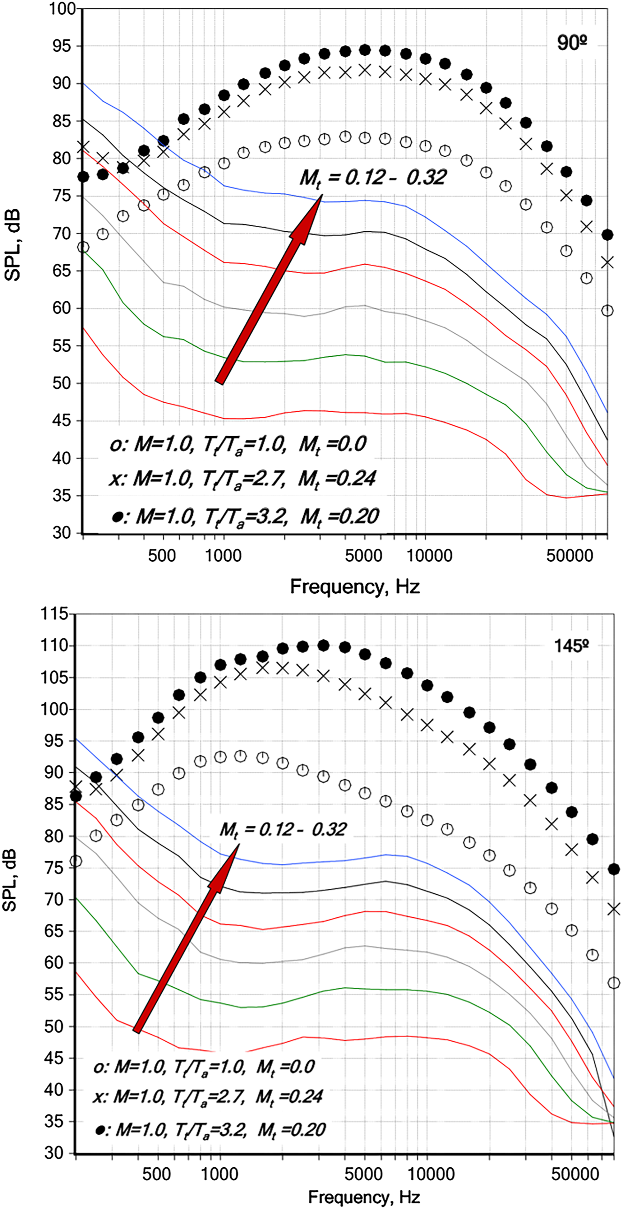

A single example that highlights the effects of forward flight for heated jets, with tunnel Mach numbers of 0.0, 0.12, 0.16 and 0.20, is shown in Figure 34. The jet operating condition is M = 0.9, T_t/T_a = 2.7. Lossless processed data are shown; the raw frequencies are used on the x-axis for the time being. The proper non-dimensional frequency for scaling the spectra is addressed next. The arrow indicates the direction of increasing M_t. The expected monotonic decrease in levels with increasing M_t is observed at all angles; furthermore, the reductions in levels are fairly uniform at all frequencies.

Figure 34.

Effect of forward flight on spectra. M = 0.9, T_t/T_a = 2.7. ●: Mt = 0.0; x: 0.12; o: 0.16; ∆: 0.20.

A relative-velocity exponent (or a flight velocity exponent), based on the measured OASPL, can be calculated from the measured data at each angle. The measured reduction in OASPL is plotted against the parameter [10 * Log10 (V_j/(V_j – V_t))]; here, V_j is the jet velocity and V_t is the tunnel velocity. Least-squares fit through the data yields the value of the exponent. The entire database has been processed and the values of the relative velocity exponent (k) at all angles have been determined. A cautious approach vis-à-vis interference by tunnel noise at the lower frequency regime has been adopted; this issue is critical especially (1) at the lower radiation angles where jet noise levels are low; and (2) for lower velocity jets at the higher tunnel Mach numbers. In practice, the measured spectra together with the tunnel noise floors have been examined at every angle and every jet condition. Whenever the tunnel noise floor led to an upturn in spectra at the lower frequencies, the spectra at that tunnel Mach number was not included in the computation of the relative velocity exponent. For example, spectra at only the lowest four tunnel Mach numbers might be included at 60° for an unheated jet with M = 0.9, whereas the data obtained at six or seven tunnel Mach numbers might be included at aft angles for a jet with M = 0.9 and T_t/T_a = 3.2. Thus, data corrupted by tunnel noise are simply ignored.

A single sample curve fit is shown in Figure 35. Three different aft angles and three different jet conditions are chosen in Figure 35. Least square fits through the measured values are also plotted in the figure. Good linear variations are exhibited by the measured data points. The values of the exponents are 7.41, 7.98, and 7.32 at 135°, 145° and 150°, respectively. It is pointed out that the values for the exponent can change slightly, by ∼ 0.25, depending on the data points included in the curve-fits. Similar linear trends are observed at other radiation angles. The variations of the flight velocity exponent with radiation angle for eight jet conditions are shown in Figure 36. The first striking observation is the following: the values of the relative-velocity exponent at different jet conditions do not have a strong dependence on jet Mach number or temperature ratio, and are tightly clustered at each angle. The dashed red line denotes a mean trend line through the values. Secondly, there is a distinct variation with angle: a slow increase from ∼2.9 to ∼3.5 at the lower polar angles from 50° to ∼105° and a steeper increase from ∼3.5 to ∼7.6 from ∼105° to 150°. There is remarkable similarity between the directivity curves for the relative-velocity exponent and the velocity exponent for turbulent mixing noise seen in Figure 22: slow variation at the lower polar angles and a steep increase in the aft quadrant.

Figure 35.

Curve-fits for the relative-velocity exponent at large aft angles.

Figure 36.

Variation of the relative-velocity exponent with radiation angle; many jet conditions.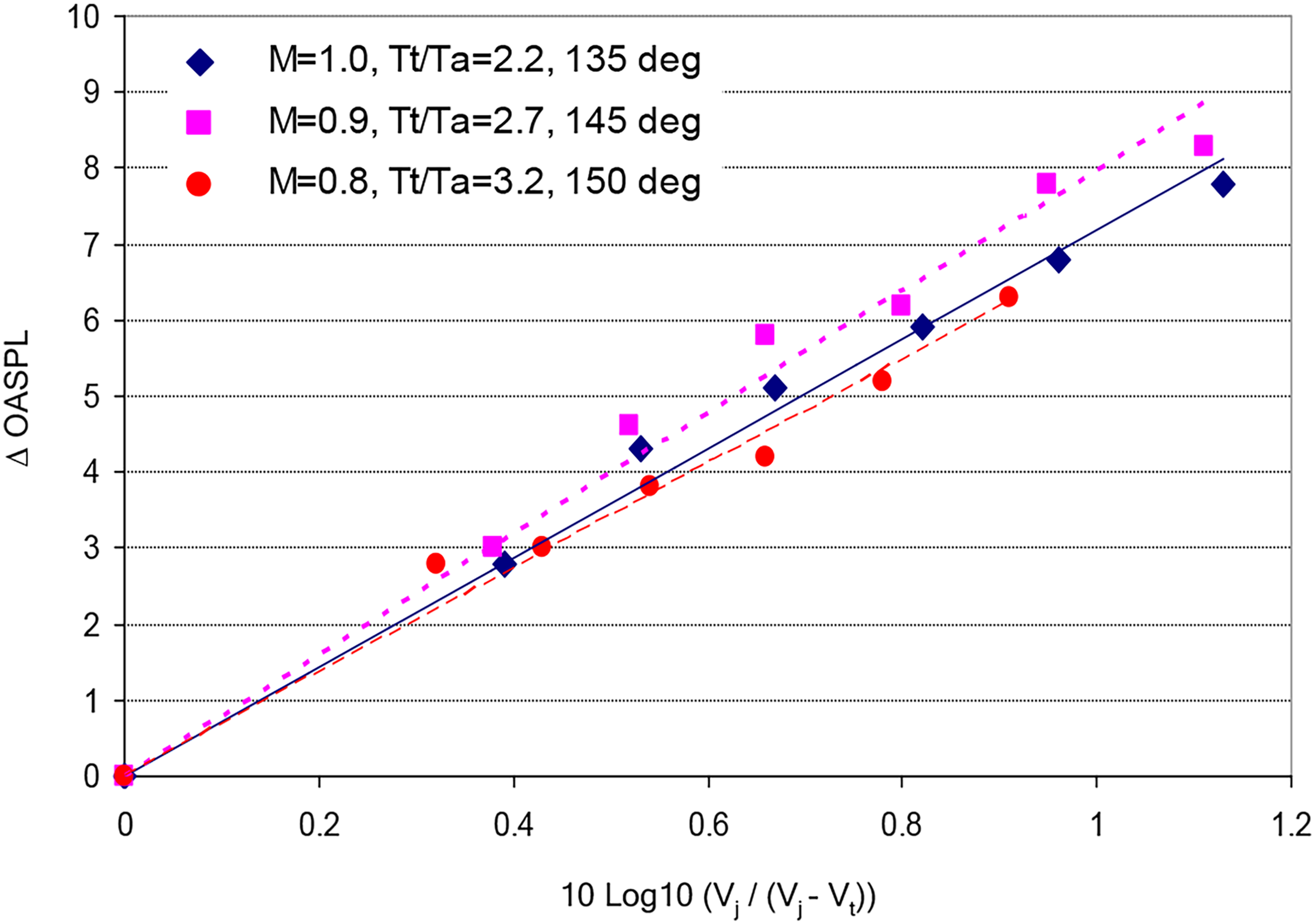

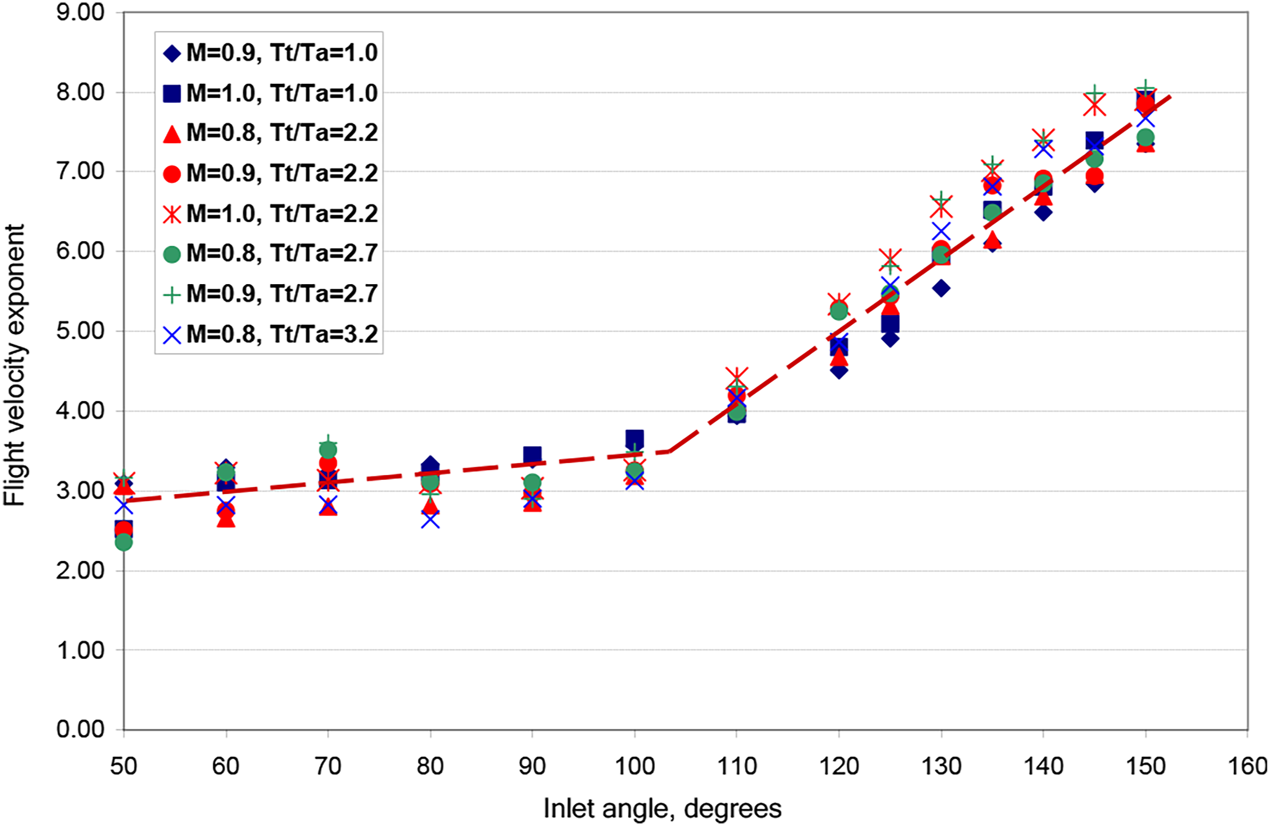
Now we demonstrate that the spectra at various tunnel Mach numbers can be collapsed with the calculated relative-velocity exponents. Recall that the raw frequency is used on the x-axis for the spectral plot shown in Figure 34. There are two choices for the non-dimensional frequency: the regular Strouhal number based on jet velocity and a modified Strouhal number based on the relative velocity. These two may be written as

S t = \frac{f D}{V_{j}}

(8)

S t_{m} = \frac{f D}{(V_{j} - V_{t})}

(9)

D is the jet diameter and f is the frequency in Hertz. The suitability of both of these is examined below. Figure 37 depicts normalized one-third octave spectra at 145° plotted against the regular Strouhal number. The jet conditions are M = 0.8 and T_t/T_a = 3.2. The quantity [SPL + 10 * k * Log10 (V_j/(V_j – V_t)] is plotted on the y-axis. Note that the normalization term is added to the raw SPL because the change in noise due to the tunnel flow (which is actually a reduction) is taken to be a positive quantity in the computation of the flight velocity exponent.

Figure 37.

Normalized one-third octave spectra at 145°. M = 0.8, T_t/T_a = 3.2. o: M_t = 0.0; x: M_t = 0.12; ●: M_t = 0.16; □: M_t = 0.20; ∆: M_t = 0.24; ▲: M_t = 0.28; 2: M_t = 0.32.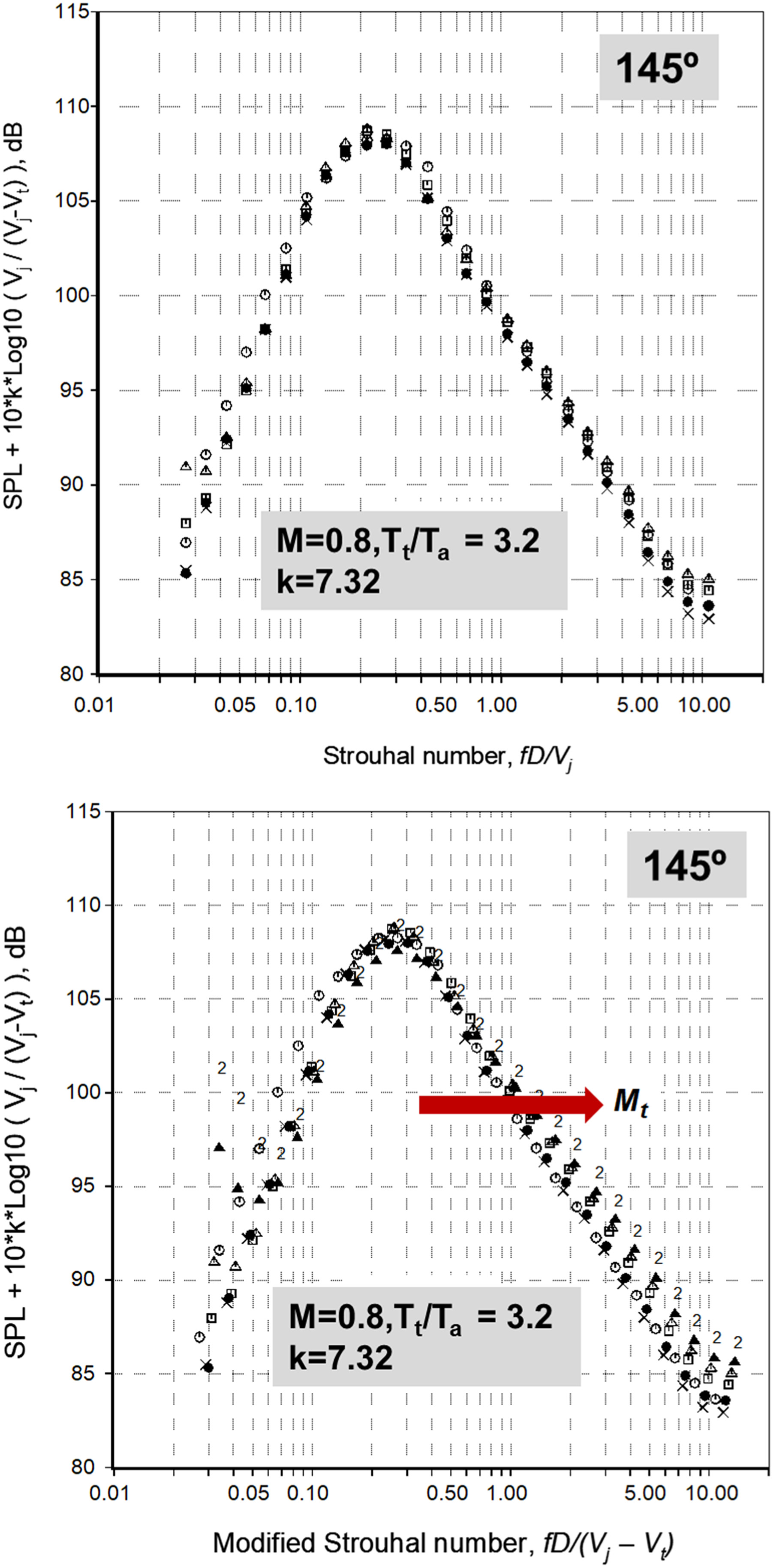

Two plots, with the regular Strouhal number (top) and the modified Strouhal number (bottom) are shown in Figure 37. There is good agreement for the normalized spectra with the regular Strouhal number, except at the highest three one-third octave bands, where a scatter of ± 1.0 dB is observed. An examination of the normalized spectra in the bottom plot indicates that the use of the modified Strouhal number based on (V_j – V_t) would destroy the spectral collapse because the spectra obtained at different (V_t) would move to the right by differing amounts. Most of the past studies have used the modified Strouhal number as the non-dimensional frequency; for example, the SAE⁸⁷ prediction method (1994), incorporates the modified Strouhal number. It has been shown conclusively here and in Figures 13 and 14 and Figures 28–31 in Viswanathan and Czech⁸⁴ that the regular Strouhal number is the correct non-dimensional frequency for scaling spectra from jets with forward flight.

Normalized spectra at another jet condition of M = 1.0 and T_t/T_a = 2.2 against the regular Strouhal number at 120° are shown in Figure 38. Spectra at all seven tunnel Mach numbers of 0.0, 0.12, 0.16, 0.20, 0.24, 0.28 and 0.32 are included. The increasing level of interference from the tunnel noise floor with increasing M_t is obvious at the lower frequencies; both the magnitude and the affected frequency range become pronounced with higher M_t. Apart from this trend, one can observe excellent collapse in the frequency range St ≥ ∼0.08. Attention is drawn to another aspect of data collapse: the flight velocity exponent has been calculated using only data uncorrupted by the tunnel noise floor (at lower M_t). However, spectra at higher M_t are also shown. Given the excellent collapse at the higher frequencies not subject to contamination by tunnel noise, it is obvious that the calculated values for the flight exponents are accurate and are applicable over a wider range of tunnel Mach numbers.

Figure 38.

Normalized one-third octave spectra at 120°. M = 1.0, T_t/T_a = 2.2. o: M_t = 0.0; x: M_t = 0.12; ●: M_t = 0.16; □: M_t = 0.20; ∆: M_t = 0.24; 1: M_t = 0.28; 2: M_t = 0.32.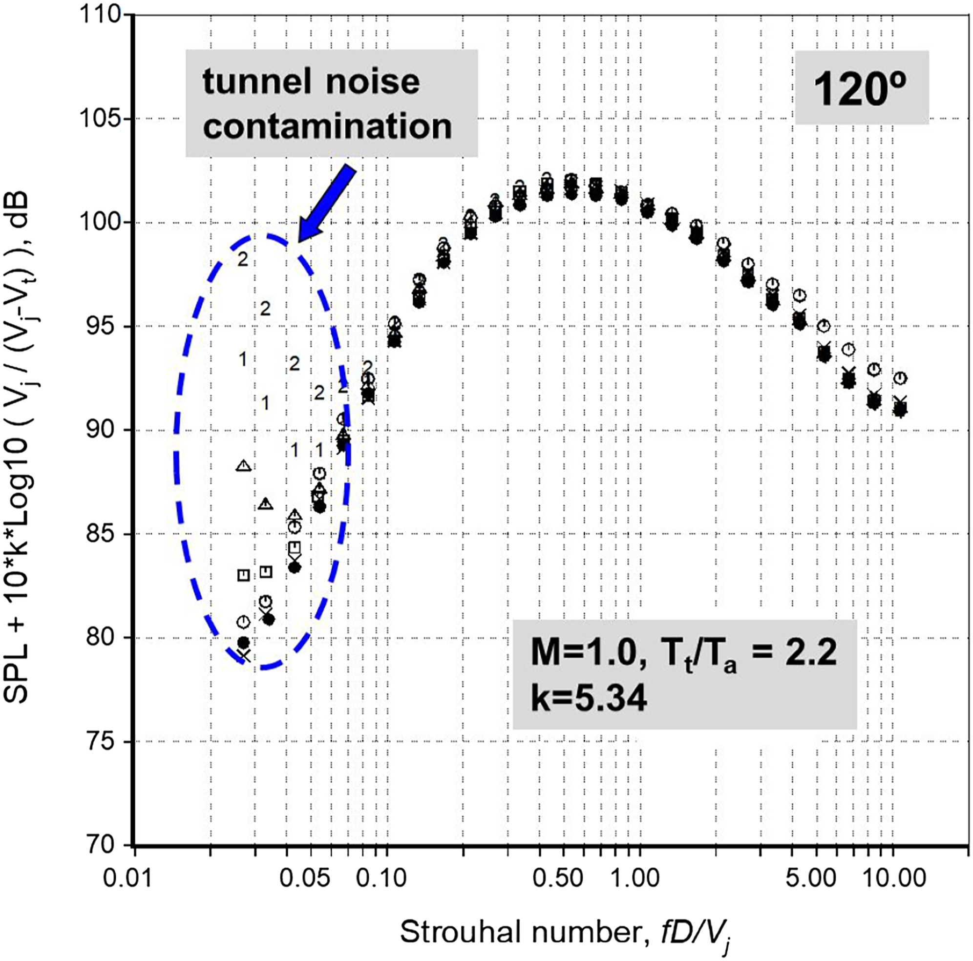

The scaling methodology developed here, see equation (7), is restricted to static jets. Now, the scaling formula can be extended to jets in the presence of forward flight. The first step involves a static “prediction”. The results presented in this paper have established that the parameter [SPL + 10 * k * Log10 (V_j/(V_j – V_t)] collapses spectra from jets with forward flight. The second term provides a “flight effect” that must be applied to the predicted static spectra, so as to obtain spectra in the presence of forward flight. This procedure can be written as:

S P L (θ, S t, V_{t}) = F (θ, S t, \frac{T_{t} o r T_{j}}{T_{a}}) {[\frac{V_{j}}{a}]}^{n} - 10 \times k \times Log 10 [\frac{V_{j}}{(V_{j} - V_{t})}]

(10)

n = n (θ, \frac{T_{t} o r T_{j}}{T_{a}}), k = k (θ)

The values of the velocity exponent n and the spectrum function F, as a function of angle and temperature ratio, are already available. The values of the flight velocity exponent (k) at each radiation angle have been determined from the current database and already presented in Figure 36. Note that k does not have a dependence on the temperature ratio or jet Mach number; no discernible trend could be established and the deviations from the mean line may be attributed to experimental scatter. An examination of Figure 36 indicates that the scatter is within ±0.5 of the mean line, with a tighter collapse at the lower radiation angles.

It is quite amazing that the characteristics of the mixing noise spectra at all angles, with or without the presence of forward flight, can be represented by a single equation. This fact is all the more remarkable as no questionable assumptions have been invoked in the development of the above equation. A complete method for the prediction of turbulent mixing noise with flight effects is now available. A notable feature of the prediction method is highlighted: because the prediction originates with a static spectrum, unaffected by tunnel noise floor (especially at the lower frequencies), the predicted flight spectrum is devoid of the turn-up at the lower frequencies due to tunnel noise (as seen in Figure 38 at higher M_t). That is, the proper spectral shape is maintained over the entire frequency range for the spectrum with forward flight. Therein lies the versatility, strength and usefulness of the prediction method: it is possible to make predictions of static jet spectra at low jet velocities, where it would be difficult to make clean measurements. It would be well-nigh impossible to measure flight effects for low velocity jets, given the additional interference from tunnel noise. It is worth noting that the plain Strouhal number, without any Doppler shift or calculated using the relative velocity (V_j – V_t), appears in equation (10), and represents the correct non-dimensional frequency for turbulent mixing noise.

Evidence for two sources of turbulent mixing noise

There is no consensus on the sources of jet noise; this point has been made amply clear. The acoustic analogy requires the description of the two-point space-time correlation of the entire turbulence field, which is difficult if not impossible to measure. There have been several attempts in the past, with different measurement techniques, to quantify the stress tensor. These have concentrated on both single-point measurements and two-point correlations of the different fluctuating quantities of turbulence within the jet plume. A second approach has consisted of measuring the correlations of the flow fluctuations with the farfield noise spectra; a variety of measurement techniques have also been adopted. Several interesting results have been obtained from these measurements: the variation of the correlation coefficients as a function of the polar angle and the azimuthal angles with jet operating conditions, the modal content of the source field, the axial and the radial location of the dominant source (either on the jet axis or the peripheral shear layer), the onset of Mach wave emission, etc.

Other techniques have also been employed for source measurements since the 1960s. An interesting test set-up to estimate the noise produced by different slices of a jet is the so-called “wall isolation” technique, first introduced by Potter⁸⁸ and further refined by MacGregor and Simcox.⁸⁹ The jet is progressively retracted behind a wall and into an insulated test cell in small incremental steps. Microphones are located downstream of the solid wall, with measurements of the noise produced by the exposed jet at various radiation angles. Thus, the difference between two successive measurements yields the noise emitted by the length of the jet retracted. Microphone array techniques have also been used in source investigations since the 1970s: the acoustic telescope of Billingsley and Kinns,⁹⁰ the polar correlation technique of Fisher et al.,⁹¹ and several phased array measurements more recently.

There have also been several near-field measurements of pressure, with the goal of identifying the acoustic or propagating components of pressure. Analyses of the spectra, from near-field circular arrays at various axial locations downstream of the nozzle exit plane, with various signal processing techniques have yielded information about the possible source fields. Many studies in the past have indicated that the lowest order modes dominate the near field of a jet. In a different approach adopted in the early 1970s, ellipsoidal and spheroidal dish-microphone systems were used for mapping the aeroacoustic noise sources.

Viswanathan^92,93 provided a brief review of the various techniques and several references; it is not possible to cite all of these here. Here is a small and partial list of these (apologies to the numerous researchers not cited here): Potter,⁸⁸ MacGregor and Simcox,⁸⁹ Grosche,⁶⁵ Siddon,⁹⁴ Seiner and Reethof,⁹⁵ Maestrello,⁹⁶ Billingsley and Kinns,⁹⁰ Laufer et al.,⁹⁷ Fisher et al.,⁹¹ Armstrong et al.,⁹⁸ Fuchs,⁹⁹ Juve et al.,¹⁰⁰ Bonnet and Fisher,¹⁰¹ Schaffar,¹⁰² Ahuja et al.,¹⁰³ Panda et al.,^104–106 Bridges and Wernet,¹⁰⁷ Jordan et al.,¹⁰⁸ Doty and McLaughlin,¹⁰⁹ Bridges¹¹⁰ and the references therein. Jordan¹¹¹ provided a compilation of the analysis techniques for source identification. It is important to recognize that no particular technique is perfect; there are advantages and limitations associated with all of these approaches with regard to resolution, assumptions involved in the interpretation of the data, requirement for à priori knowledge of the source characteristics, omni-directivity of the noise sources, etc., as noted by Fuchs.⁹⁹ However, the collective information gleaned from these source measurements has proved to be valuable.

Here, we employ several approaches to establish the presence of two distinct sources of noise from very low to high jet velocities. Viswanathan^92,93 and Viswanathan et al.¹¹² utilized four techniques: (1) examination of farfield spectra; (2) azimuthal and polar correlation of farfield spectra; (3) source distribution measurements with an elliptic mirror; and (4) near-field source measurements and correlations of nearfield and farfield spectra. In a collaborative effort, Tam, Viswanathan, Ahuja and Panda¹¹³ compiled the available data obtained with four different approaches, especially with regard to high-speed jets. These consisted of (1) analyses of farfield spectra, (2) farfield correlations to uncover the spatial structure of the sources, (3) correlations of turbulent fluctuations inside the jet and farfield spectra, and (4) the measurements of source distributions using the elliptic mirror. Data for the joint analyses came from the current database, from Seiner et al.,¹¹⁴ Norum and Brown,¹¹⁵ Georgia Tech Research Institute, and Panda et al.^104,105. Salient results are presented now.

Spectral shape at large aft angles from low-velocity jets

First we concentrate on low-velocity jets and their spectral shapes at angles close to the jet exhaust axis. The following results form a sub-set of results from Viswanathan.⁹³ Figure 39 shows comparisons of the LSS spectrum with measured spectra from unheated jets at 160°; the Mach numbers are 0.4, 0.5, 0.6, 0.7, 0.8, 0.9 and 1.0. The maximum spectral level associated with each curve is also indicated. There is excellent agreement even at the lower Mach numbers of 0.4 (440 ft/s) and 0.5! Recall that the shape of the LSS spectrum was extracted from supersonic spectra. Note that the spectral peak occurs at a fixed frequency at all Mach numbers; this peculiar feature for unheated jets was first reported by Lush.⁷⁸

Figure 39.

Comparison of measured spectra with large-scale similarity spectrum. Unheated jets. D = 2.45″, angle = 160. ■: M = 0.4; o: M = 0.5; □: M = 0.6; Δ: M = 0.7; x: M = 0.8; •: M = 0.9; +: M = 1.0.

Next, spectra at ultra-low velocities have been considered; the measured narrowband spectra along with the noise floor at an angle of 165° are shown in Figure 40. The noise floor is made up of the sum of the ambient noise and the electronic noise, and is denoted by the thick black line at the bottom. The microphone had to be located close to the jet exhaust collector for this large angle; reflections from the collector lip are unavoidable. The jet Mach number is progressively increased and the spectra for jets with M = 0.21, 0.24, 0.26, 0.29, 0.31, 0.33, 0.35, 0.41, 0.45 and 0.60 exhibit the expected monotonic increase in level. The spectrum for the noise floor peaks at 200 Hz, decreases as the frequency is increased, and flattens out with a level between ∼10 dB and ∼15 dB for the frequency range of ∼3 kHz to 80 kHz. The spectrum for the M = 0.21 jet is very close to the noise floor for most of the frequencies. As the Mach number is increased, there is an enlarging separation between the measured levels and the noise floor at the lower frequencies, which is ≥ 6 dB for M >0.26. However, at the higher frequencies, the measured data eventually run into the noise floor, due to the spectral shape and the effect of atmospheric absorption which increases with frequency and can reach ∼ 1 dB/ft at 80 kHz. When the narrowband spectra are synthesized to produce one-third octave spectra, there is a tail-up at the higher frequencies because of the contamination due to the noise floor and the ever-increasing bandwidth with frequency. This point should be kept in mind when the following figures are examined. (As an aside, it is obvious that it would be impossible to measure noise at low velocities, even in excellent facilities as seen in Figure 40. The overall sound pressure levels in the forward quadrant and lower angles are ∼8 dB below the value in the peak radiation sector of ∼165°, for low velocity jets. The possibility of measuring clean noise at lower angles is entirely hopeless. One should be leery and sceptical about accepting any conclusions).

Figure 40.

Measured spectra from unheated jets at 165°. M = 0.6, 0.45, 0.4, 0.35, 0.33, 0.31, 0.29, 0.26, 0.24, 0.21.

The one-third octave spectra at 165° are collapsed in Figure 41; data at two higher Mach numbers of 0.6 and 0.7 (denoted by numbers) are also included for the sake of comparison. There is excellent agreement between the spectra and the LSS over the entire frequency range for these higher M. It is clear that the spectra at the lower M (0.24 to 0.4) also conform to the LSS shape in the frequency range not impacted by the noise floor. The shaded region highlights the higher frequencies that are corrupted; for the M = 0.4 jet (dark squares) the demarcating frequency is ∼ 30 KHz as seen in Figure 40. At lower Mach numbers, the region of contamination gets wider progressively, as identified by the tail-up and the increasing mismatch with the LSS shape. As expected, the noise from the M = 0.24 jet (crosses) is subject to the most contamination. The problem with the rig internal noise at the lower frequencies is also evident.

Figure 41.

Spectral collapse from unheated jets. Solid line: large scale similarity spectrum. Symbols: one-third octave data. 2: M = 0.7; 3: M = 0.6; ▪: M = 0.4; Δ: M = 0.35;□: M = 0.33; ▲: M = 0.31; +: M = 0.29; ●: M = 0.26; x: M = 0.24.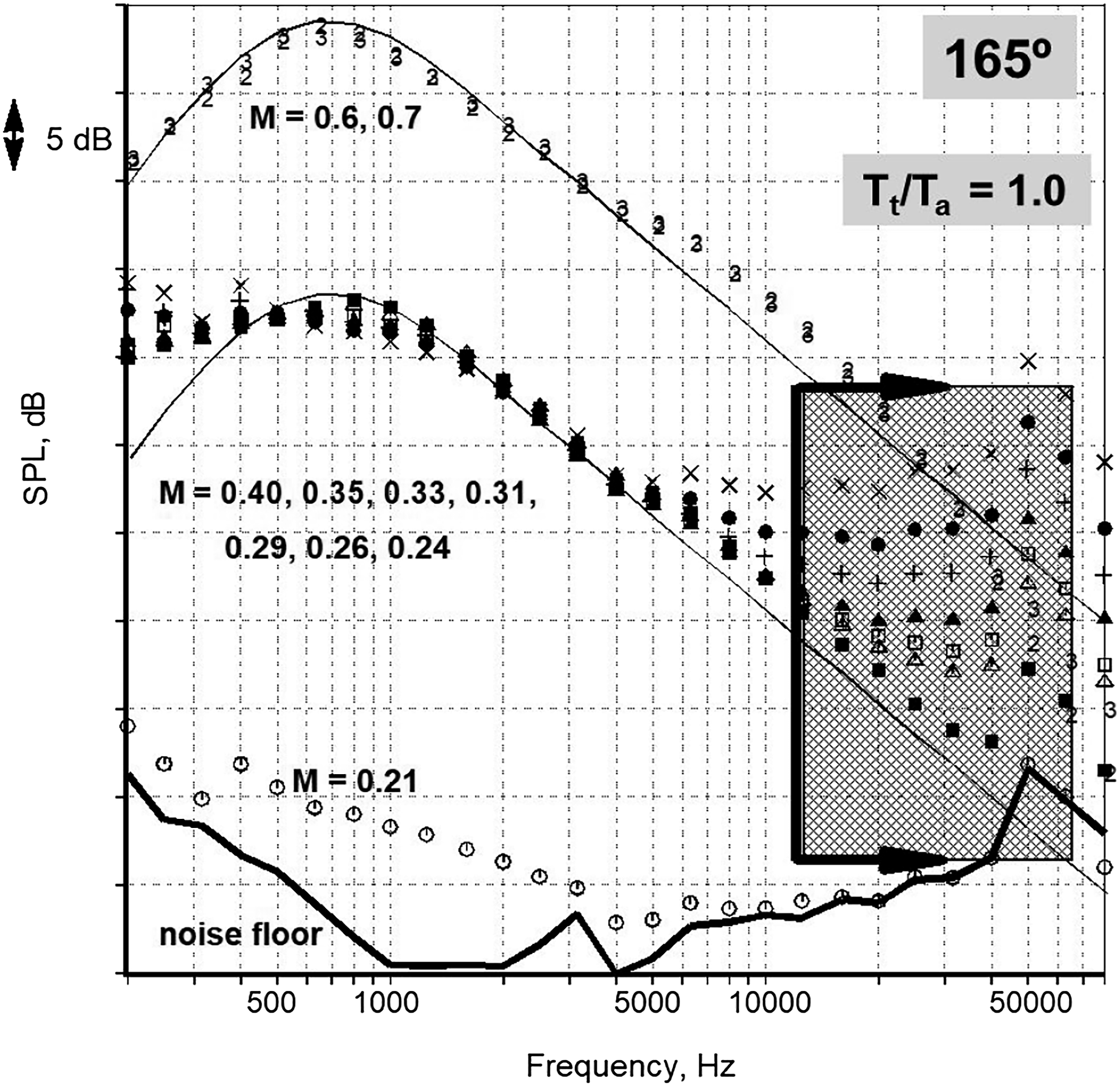

It was established that the spectra at 90° and at lower angles have a universal shape; the spectral shape at large aft angles are completely different from the shape at 90°. The paramount conclusion from the above example and a comprehensive exercise in Viswanathan⁹³ is that the spectra attain the LSS shape for all jet velocities, at angles close to the jet axis. This trend seems to be a fundamental characteristic of turbulent mixing noise. This is a surprising new finding. Recall that Tam et al.³⁶ extracted the similarity shapes from highly heated supersonic jets; the convective Mach numbers (M_c, taken to be ≈ 70% of V_j/a) for these high-speed jets are supersonic. In contrast, the convective Mach number for the M = 0.24 jet is only ∼0.17.

Viswanathan⁴⁵ proposed that the noise from large-scale structures could be a factor even for low speed jets and pointed out that the instability waves at low Strouhal numbers amplify more gradually than waves at high Strouhal numbers, and attain their peak amplitudes close to the end of the potential core. In addition, instability waves for low velocity jets have higher growth rates than those of high-speed jets. Just beyond the potential core, these waves have no mechanism to extract energy from the mean flow and lose their energy through nonlinear processes; see Ffowcs-Williams and Kempton,²⁵ Tam and Burton,²⁹ and Morris.¹¹⁶ This process would occur over a region that is a few diameters in extent, downstream of the end of the potential core. The modulation of the amplitude of the instability waves due to the growth/decay cycle could trigger low-wavenumber components with potentially supersonic phase speeds relative to the ambient speed of sound. Given the low velocities, though, this radiation would be confined to angles close to the jet axis; see also Tam et al.¹¹³. Thus, the large-scale structures could be a source of noise for low velocity jets as well. The physical process outlined here could also explain the puzzling observation of why the LSS shape, extracted from jets with velocities of 3450 ft/s (1050 m/s) is seen for such a low velocity jet (270 ft/s).

The farfield shapes of FSS at low angles and LSS at aft angles have already been presented here and in several papers by Tam and Viswanathan, both for subsonic and supersonic unheated and heated jets. The importance of these two sources have been calculated in the transition region by decomposing and fitting both shapes so that they add up to the measured spectra, as notionally shown in Figure 5 here and in several quantitative examples in Tam et al.¹¹³. The directivity of the OASPL over a large range of Mach numbers and two temperature ratios of 1.0 and 2.2 are reproduced here as Figure 42. The solid circles denote the noise from fine scale turbulence and the open circles are those of the noise from large turbulence structures. This figure shows clearly that the large turbulence structures noise is highly directional and drops off rapidly around θ = 120° to 140°. This characteristic is consistent with Mach wave radiation for high speed jets with a sharp cut-off around the Mach wave angle. The fine scale turbulence noise increases gradually with θ. At a fixed Mach number, the exit velocity is higher for the heated jet. As a result, one would expect stronger Mach wave radiation for jets at a high temperature. This increase in noise radiation with jet temperature can easily be seen by comparing these two plots. Also, for the same reason, the disparity in the noise intensity radiated by the large turbulence structures and that by the fine scale turbulence becomes larger for hot jets; this difference becomes more pronounced at higher jet Mach numbers. Thus, the directional dependence of the noise components are very different.

Figure 42.

Variation of OASPL with radiation angle. Top: T_t/T_a = 1.0, bottom: T_t/T_a = 2.2. Dark symbols: contributions from fine-scale turbulence; open symbols: from large-scale turbulence.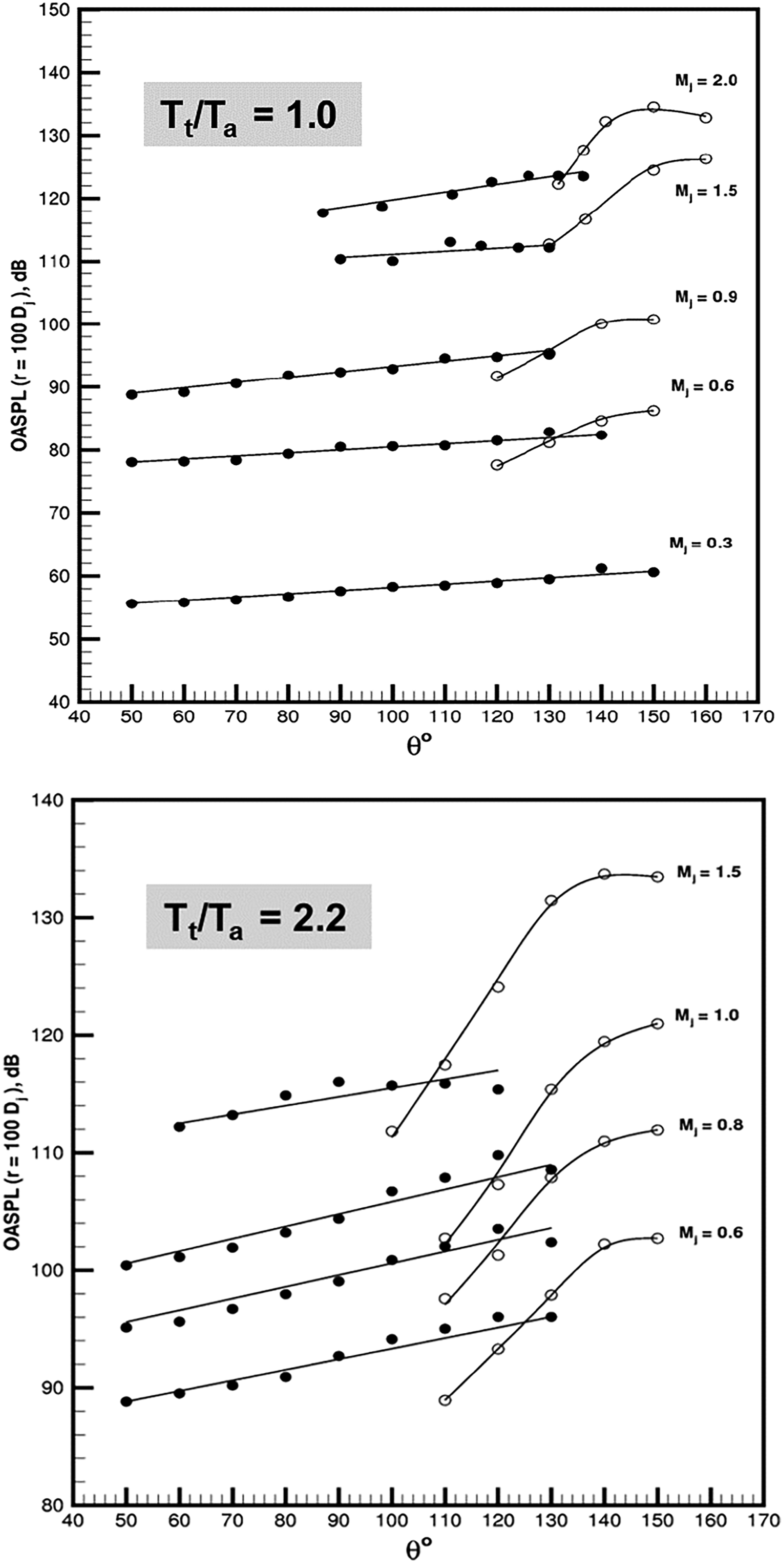

Next we examine the angular variation of the peak Strouhal number [St_peak = f_pD_j/u_j where f_p is the frequency at the spectrum peak] extracted from narrowband spectra, at two Mach numbers of 0.6 and 1.0. Figure 43 shows the trends: the temperature ratios are 1.0, 1.8 and 2.7 for M = 0.6, and 1.0, 2.2 and 3.2 for M = 1.0, respectively. In the directions for which fine scale turbulence noise is dominant, St_peak increases slowly with polar angle. In the directions for which large turbulence structures noise dominates, the trend is totally different. The peak Strouhal number decreases rapidly with increasing angle and appears to be insensitive to jet temperature. A comparison of the two plots indicates that the peak Strouhal number is slightly higher for the M = 0.6 jet at the lower angles for the fine-scale turbulence. However, for the large turbulence structures noise, the peak Strouhal number is relatively independent of Mach number and temperature, as already seen in Figures 26–28.

Figure 43.

Variation of peak Strouhal number with angle. Top: M_j = 0.6 ●,▽ T_t/T_a = 1.0, ■, ○ T_t/T_a = 1.8, ▲, △ T_t/T_a = 2.7. Bottom: M_j = 1.0. ●,▽ T_t/T_a = 1.0, ■, ○ T_t/T_a = 2.2, ▲, △ T_t/T_a = 3.2.

It was already documented that the velocity exponent for OASPL (Figure 22) and the flight velocity exponent (Figure 36) have distinctly different variations with angle: a slow increase in the forward quadrant and up to ∼100°, and a rapid increase in the aft quadrant. Figure 42 for the OASPL and Figure 43 for the peak Strouhal number also exhibit a slow increase in the same angular range. These trends are followed by a rapid increase and a rapid decrease, respectively, as we move aft. The distinctly different dependence of all these parameters on the direction of radiation leaves little doubt that there are two very different sound fields surrounding a jet, suggesting that there must be two noise sources with greatly different characteristics.

The fundamental question that remains unanswered conclusively to date is: are large scale structures important noise generators at very low jet velocities? The connection between correlations, both in the polar and azimuthal directions, and the farfield spectral shapes is examined. The modifications to the spectral shapes and the correlations due to the beveling of a round nozzle are investigated to gain further insights to the noise from the large coherent structures of the jet flow.

Azimuthal and polar correlations

Both polar and azimuthal correlations at various jet velocities are examined, especially while keeping in mind the spectral trend observed above. The aim of this exercise is to uncover any connection between the noise generation mechanisms between high-speed and low-speed jets. Measurements of the farfield correlations of jet noise have been carried out in the past, as already noted. Here, two farfield microphone arrays are deployed: a polar array which spans the angular range of 60° deg to 150°, and an azimuthal array that spans an angular range of 180°. Figure 44 shows a photograph of the two arrays. The azimuthal angle is measured counterclockwise from the bottom dead center (towards the ground), which corresponds to 0°. In order to facilitate measurements from both these arrays simultaneously, a semi-circular azimuthal array with 19 microphones at 10° degree intervals was constructed; these microphones are located at azimuthal angles from 240° to 60°. The azimuthal array was mounted on the same traversing cart/platform used for the elliptic mirror (described in later Section), thereby providing the flexibility to obtain azimuthal correlation measurements at any desired polar angle. Time-series data were recorded from all the microphones for different nozzles at several test conditions. These data have been processed to produce correlation plots and coherence spectra. The coherence function γ²(f) between any two microphones is defined by:

γ_{12}^{2} (f) = \frac{{| G_{12} (f) |}^{2}}{G_{11} (f) G_{22} (f)}

(11)

where G₁₁ and G₂₂ are the one-sided auto-spectra and G₁₂ is the cross-spectrum between the two signals. Similarly, the cross-correlation coefficient function β₁₂(τ) is defined by:

β_{12} (τ) = \frac{R_{12} (τ)}{{[R_{11} (0) R_{22} (0)]}^{\frac{1}{2}}}

(12)

where R₁₁ and R₂₂ are the autocorrelation functions, R₁₂ is the cross-correlation function and τ represents the time delay.

Figure 44.

Photograph of the polar and azimuthal microphone arrays. The jet rig and the wind tunnel are also shown.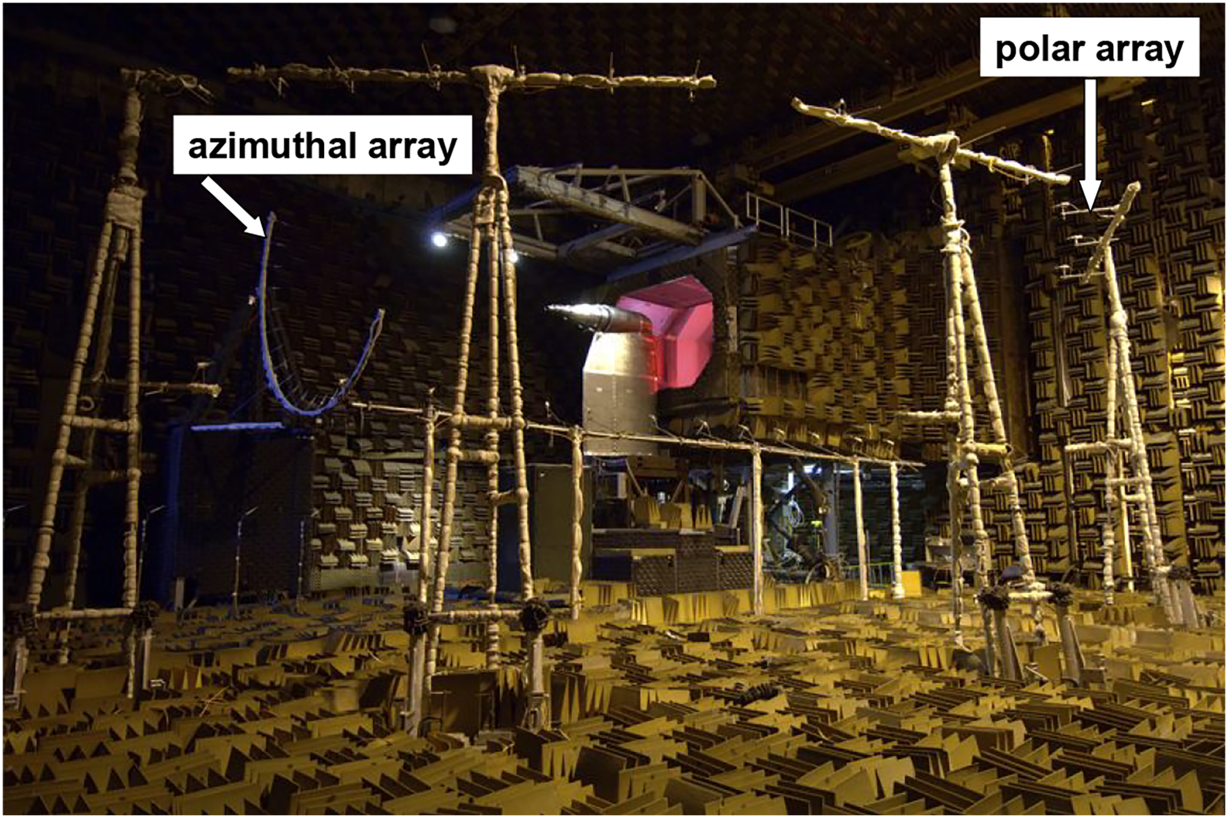

A comprehensive set of correlation results and implications may be found in Viswanathan^92,93; sample results are discussed here. First we present the correlations for a heated jet: M = 0.9, T_t/T_a = 3.2, V_j/a = 1.5. The convective Mach number is supersonic for this case. Figure 45 shows polar correlations for two different reference microphones at 150° and 90°, respectively. As the separation angle between the reference (fixed) and the second microphone is increased, the value of the maximum correlation coefficient decreases progressively. For the 150° mic, there is high correlation for an extended angular range; the coefficient drops to ∼0.2 (20%) at an angle of 125°. The trend is very different for the 90° microphone; the correlation drops to ∼0.2 (20%) when the polar separation angle is only ±10°. The correlation coefficients in the azimuthal plane for the two polar angles of 150° and 90° are shown in Figure 46. Whereas a high correlation level of ∼0.65 (65%) is maintained for a separation angle of 150° in the peak radiation direction, the levels fall below 0.20 for a separation angle of 40° when the reference microphone is at 90° and at the forward angles (not shown). Thus, the sound field at large aft angles is axisymmetric and highly correlated over 360° in the azimuthal plane.

Figure 45.

Polar correlations; M = 0.9, T_t/T_a = 3.2. Top: reference microphone at 150°; bottom: reference microphone at 90°.

Figure 46.

Azimuthal correlations; M = 0.9, T_t/T_a = 3.2. Top: azimuthal array positioned at polar angle of 150°; bottom: azimuthal array positioned at polar angle of 90°.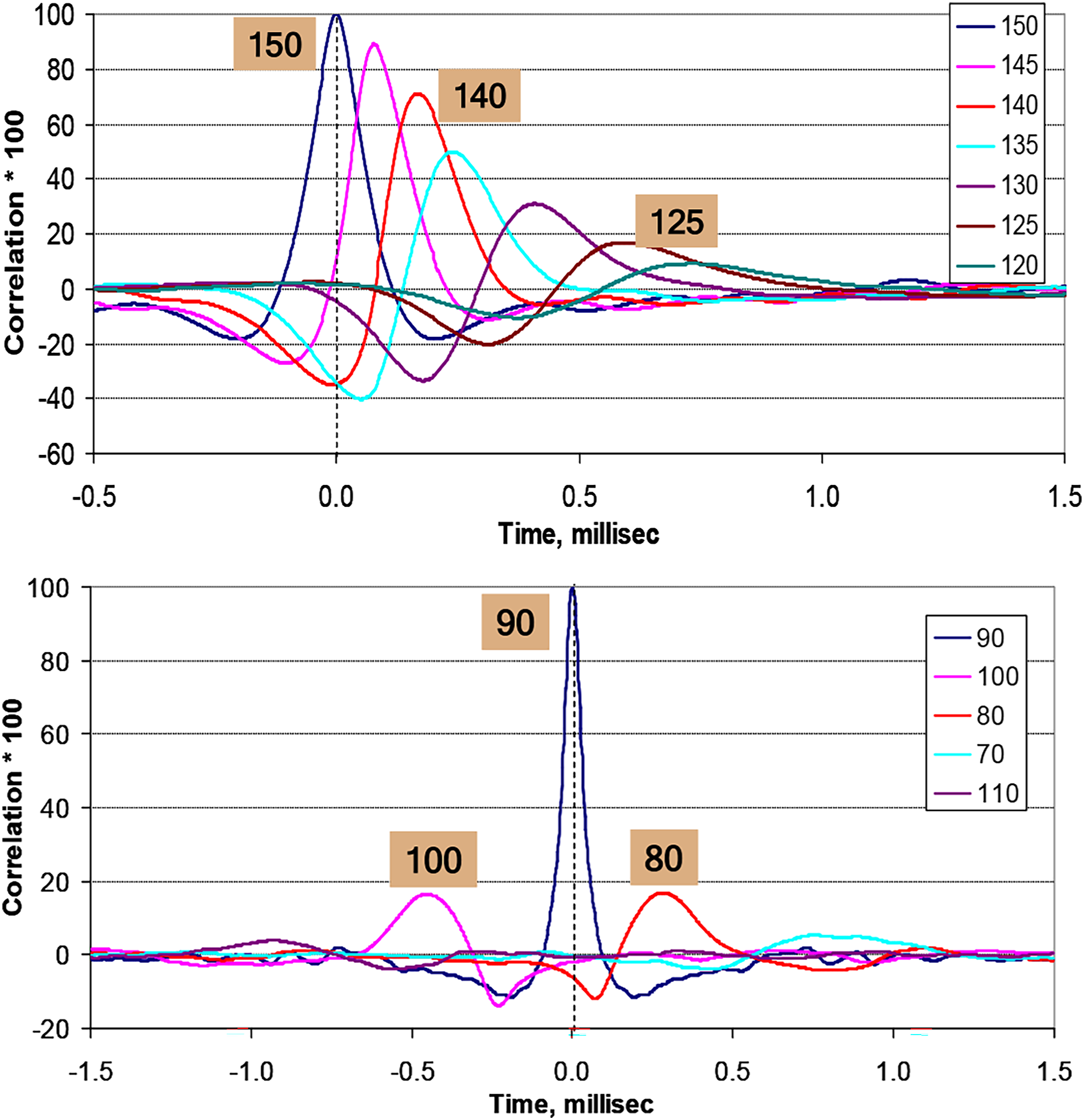

The azimuthal and polar variations of the coherence spectra when the fixed reference microphones are at 150° and 90°, respectively, are shown in Figures 8–10 in Viswanathan⁹³ and are not repeated here. When the azimuthal array is at a location that correspond to a polar angle of 150° and the reference microphone is at 270° in the azimuthal plane, two distinct features are exhibited: (1) there is a high level of coherence at the lower frequencies, ∼80% for all the azimuthal separations; and (2) the coherence level drops with separation angle as the frequency is increased. The situation is very different when the coherence functions are examined at a polar angle of 90° in Figure 10 in this reference. The correlation drops very rapidly both in the polar direction and in the azimuthal plane (below 20% for ∼40° separation) even at low frequencies.

We now turn our attention to a low velocity jet: M = 0.4, T_t/T_a = 1.0, V_j/a = 0.4. The convective Mach number is ∼ 0.28 for this case. Figure 47(a)–(c) shows the azimuthal correlations at three polar angles of 90°, 150° and 160°, respectively. [Similar plots at two additional angles of 130° and 155° are included in Figure 12 in Viswanathan⁹³]. At the lower polar angles, the maximum correlations drop to ∼0.2 (20%) for a separation angle of 50°. At a polar angle of 150°, maximum correlation levels ≥0.2 (20%) are maintained for an azimuthal separation of 120°; at 155°, there is increased peak correlation ≥0.36 (36%) for a larger azimuthal separation angle of 150°. At 160°, the peak correlations increase to ≥0.54 (54%) for all separation angles. The correlations at 160° for the low velocity jet are comparable to those for the convectively supersonic jet shown in Figure 46 in the peak radiation angle. Figure 13 in Viswanathan⁹⁴ provides the farfield spectra at four of the polar angles and comparisons with the similarity spectra. The data at the two lower polar angles of 90° and 130° conform to the FSS shape; the spectrum at 160° has the LSS shape. The spectrum at 150° is in transition from the FSS to the LSS shape and can be represented only by a combination of both shapes (notionally shown in figure).

Figure 47.

Azimuthal correlations at various polar angles; M = 0.4, T_t/T_a = 1.0. (a) 90°; (b) 150°; (c) 160°.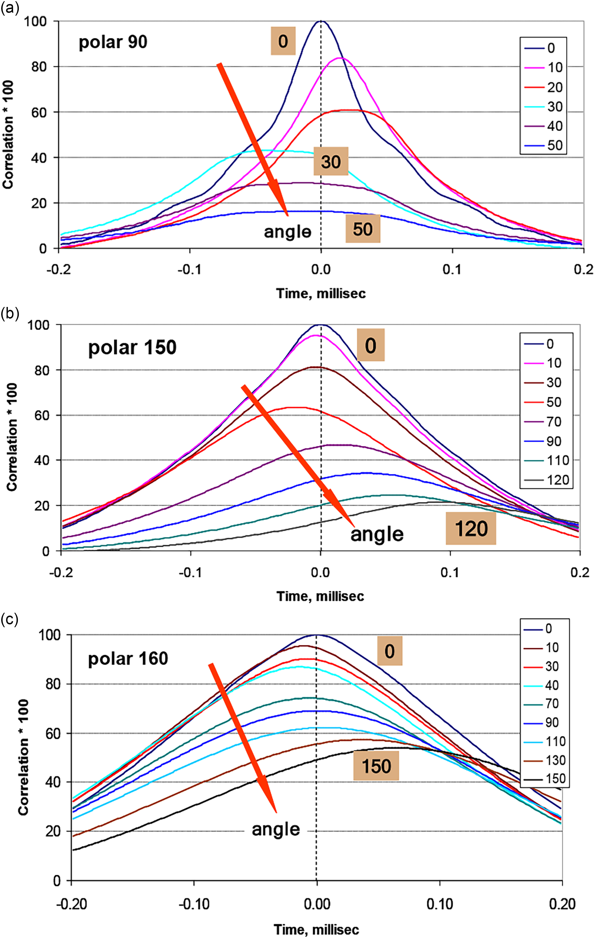

When the correlations are examined together with the farfield spectra, the following picture emerges: when the spectral shape conforms to the FSS shape, there is low correlation; when the spectral shape conforms to the LSS shape, there is very high correlation; in the transition region, the level of correlation is much higher than that seen for the FSS shape. The trends seen for the low velocity jet (V_j/a = 0.4) are remarkably similar to those for the high-speed jet (V_j/a = 1.5). However, the high correlation values as well as the LSS shape are confined to a narrow angular sector, close to the jet downstream axis.

Is there a common mechanism (growth/decay) then by which the large scale structures radiate noise at high and low velocities? This question is addressed through the examination of the variation of the peak polar correlation with separation angle for a range of low to high jet velocities. The reference microphone is at the peak radiation angle of 150°. Figure 48 shows such a variation for four test cases: unheated jets with M = 0.4 and 0.5, and two M = 0.9 jets with stagnation temperature ratios of 2.7 and 3.2. The corresponding V_j/a are 0.40, 0.49, 1.38 and 1.50, respectively. There are remarkable similarities in the trends for all the jets in spite of the vast disparity in the jet velocities. The peak correlation values are slightly higher for the high-speed jets, but not by a significant amount; high correlations levels of ∼0.18 persist down to an angle of 125°. Strong evidence has been presented here that indicates that the large scale structures are important noise generators for low velocity jets as well.

Figure 48.

Variation of the peak correlation with polar angle; reference microphone at 150°.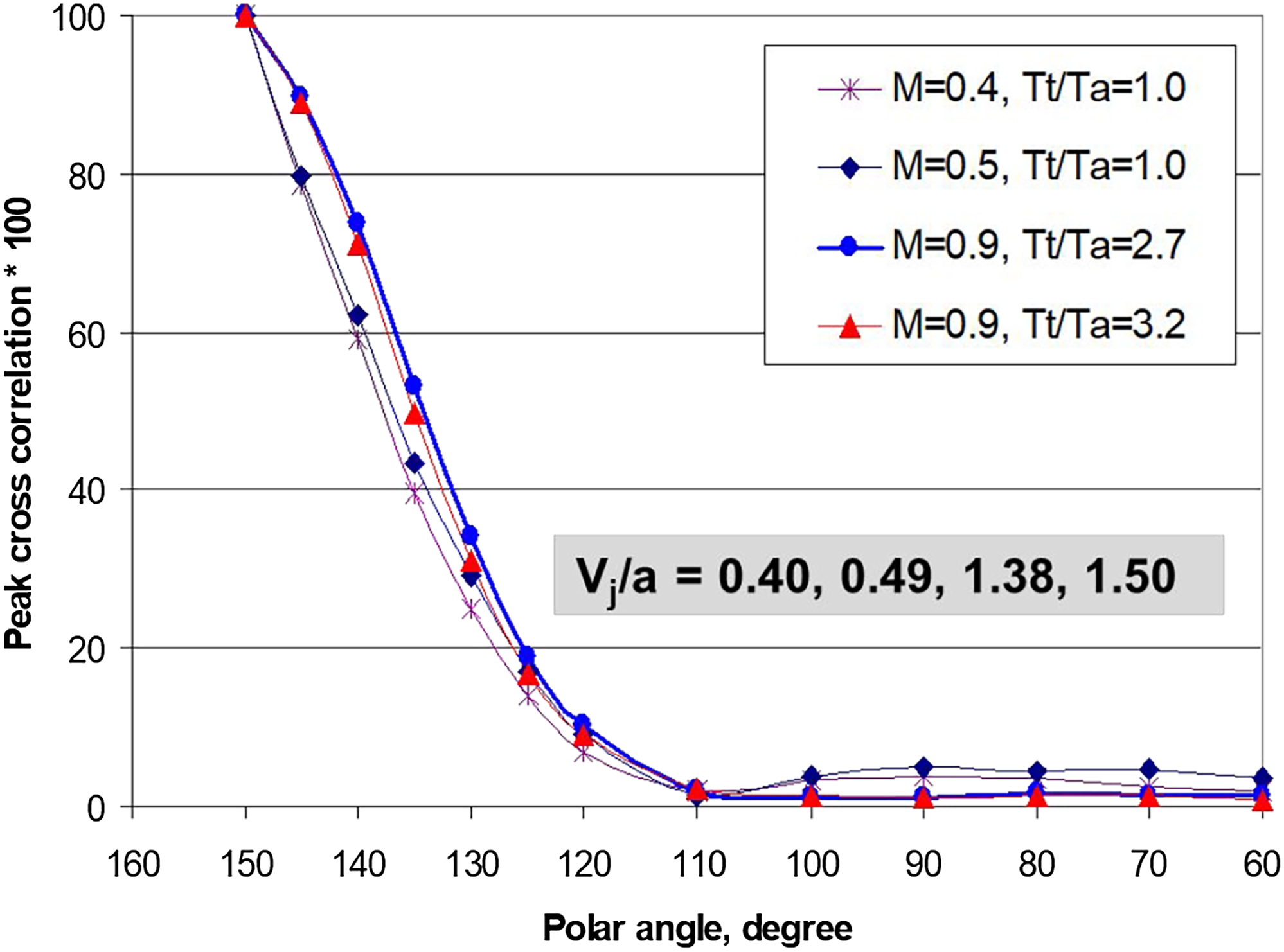

The reason for the observed similarity is explained in detail in Section 3 of Tam et al.¹¹³. The key idea is that the width of the acoustic beam in the peak radiation direction is of the order of the size of the large scale structures, thereby increasing the probability of two microphones located in the peak radiation sector measuring the same pulse and consequently leading to a high correlation level. The crucial difference between the characteristics of the normalized cross-correlation function of the sound radiated by the fine-scale and large-scale structures, is due to the width of the acoustic beam. If this is the underlying physics, then the intensity of sound would play only a lesser role. [Alternate explanations of the cross-correlations have been offered by Ribner¹¹⁷ and in the summary of the work by Michalke, provided by Michel¹¹⁸]. The above hypothesis of Tam et al.¹¹³ is validated by the trends seen in Figure 48, as the peak correlation levels are comparable for low and high speed jets and are seen to be relatively independent of sound amplitude. The results of Figure 48 suggest strongly that the mechanism by which the large structures generate noise could be the same for jets at different velocities, from very low to supersonically convective. Further investigation of this phenomenon is necessary.

For beveled nozzles, conceived specifically to alter the noise radiated by the large-scale structures, correlation measurements have been obtained to augment previous spectral data; see Viswanathan⁹³ for complete details. In contrast to the spectra from a round nozzle, which conform to the FSS shape at a polar angle of 120° for all Mach numbers and stagnation temperature ratios, the spectra from a beveled nozzle conform to the LSS shape for Mach numbers in the range of 0.6 to 1.0 at a temperature ratio of 3.2. There is a corresponding higher polar correlation for the bevel45 towards the short lip. Also, the angular range with higher correlations extends to the lower polar angles. A curious and unexplained feature is that much higher negative peaks (up to twice the value of the positive peaks) are seen only in the direction of the short lip. In the azimuthal plane, peak correlations of ∼0.7 (70%) are observed for an angular range of ±30° for the short lip; the spectra within this angular range conform to the LSS shape. In contrast, the levels of correlation are much lower for the round nozzle with the FSS shape. The correlation data confirm earlier observations that the noise from the large structures is beamed to lower polar angles towards the short lip and that the noise reduction of the beveled nozzle is due to the manipulation of the noise mechanism associated with the coherent structures. Therefore, the trends observed for the beveled nozzle bolster the concept of two independent noise sources. See Viswanathan^93,94 for additional information. Tam et al.¹¹³ provide physical reasonings for the observed characteristics of wider auto-correlation functions and larger negative peaks at large aft angles, which are insightful in understanding the trends.

The drastic difference in the nature of the dominant source responsible for noise radiation, i.e., a random incoherent source at 90° (and lower polar angles) and a highly correlated coherent source at 150° (and large aft angles) indicate strong evidence for the existence of two independent sources in both high-speed and low-speed jets. With increasing polar angle, the contributions from the large scale structures increase progressively and eventually dominate the total radiation at aft angles. The jet velocity controls the polar angle beyond which the noise from the coherent structures becomes fully dominant.

Correlation of jet turbulence fluctuations and farfield sound

A truly nonintrusive method using the Rayleigh-scattering technique for measuring turbulence fluctuations in high speed jets was developed and perfected at the NASA Glenn Research Center by Seasholtz, Panda and Elam^119,120 that eliminated many restrictions with the past use of hot wires, LDV, etc. Panda et al.^104,105 and Panda¹⁰⁶ correlated this new set of flow measurements with farfield spectra at several polar angles, to gain insights to the noise sources. An extensive set of data of density and velocity fluctuations and farfield spectra was acquired simultaneously from unheated and heated subsonic and supersonic jets. The laser probe volume (for Rayleigh-scattering measurements) was traversed on an (x, r)-plane (x: axial, r: radial directions) containing the jet centerline, down the jet column for many axial diameters downstream, while the microphone was kept fixed at a particular polar angle.

Tam et al.¹¹³ carried out detailed analyses, by normalizing the correlation data by a common reference value (denoted by subscript ref), because the absolute level of the correlation function is a measure of the noise source strength. Thus, the normalized data are used to identify dominant noise source location, relative strength and directivities. Sample results are highlighted here. Figure 49 shows directivity plots of the maximum measured normalized correlations. The laser probe was kept fixed at the centerline of the jet at x/D = 12 for the Mach 1.8 jet and x/D = 10 for the Mach 1.4 and Mach 0.95 jets. The far-field microphone was moved at 10° intervals on a circular arc. The top figure shows the directivity of the normalized ‹ρuu, p′›_max/[(ρuu) _rms ( p′) _rms)] and the bottom ‹ρ′, p′›_max/[ρ′_rms p′_rms]. Here, a prime represents the deviation from the mean. There are significant correlations between the turbulence fluctuations at a point inside the jet and the sound field radiated in the downstream direction. This is true regardless of which turbulence-related fluctuation is used. Since the Rayleigh scattering measurements are concentrated in a very localized volume in the jet, a 20% correlation is a huge number. The normalized correlation drops off rapidly as the inlet angle decreases; for angles less than 120°, the correlation practically diminishes to an insignificant level. These directivity patterns do not change when the laser probe is moved radially over the half-width of the jet and axially over a few jet diameters, indicating that the direct correlation function and noise sources are highly directional. There is strong directional beaming of noise only to the downstream angles and practically no radiation to angles less than ∼120°.

Figure 49.

Directivity of normalized ‹ρuu, p′›_max correlation (top) and ‹ρ′, p′› _max correlation (bottom). Laser probe locations are at r/D = 0, x/D = 12 (Mach 1.8), 10 (Mach 1.4 and Mach 0.95).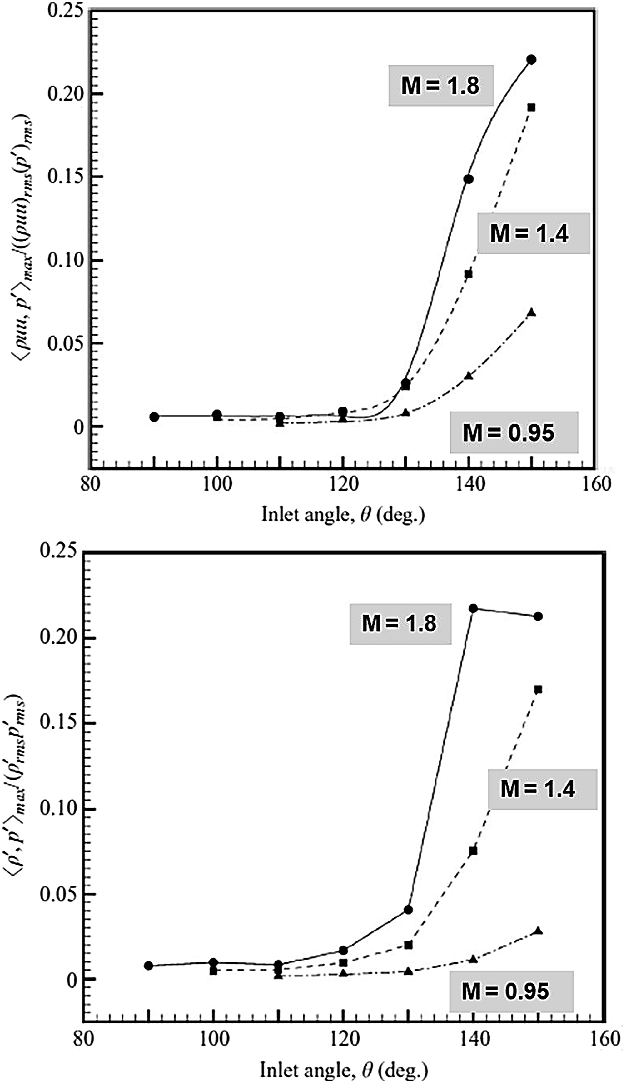

Figure 50 shows the normalized axial variation of the density–pressure correlations for four Mach 0.9 jets at temperature ratios of 1.0, 1.43, 1.82 and 2.70. The laser probe is moved along the jet centerline; the far-field microphone is at 150°. In order to bring out the effect of temperature, a common reference from the unheated jet is used for normalization. The value for [ρ′_rms] is the one at r/D = 0, x/D = 7.0 and for [p′_rms] is at 150°. As expected, the correlation values increase as the temperature increases. The peak intensity for all the cases occurs at ∼7D. Similar results along the lip line are shown in Section 4 of Tam et al.¹¹³. For a M = 1.48 jet, the peaks occur slightly more downstream, given the longer potential core length. And for a M = 0.5 jet, the peaks are closer to the nozzle exit plane. Thus, the peaks are observed downstream of the potential core for each Mach number.

Figure 50.

Axial variation of ‹ρ′, p′› _max/[ρ′_rms p′_rms]_ref. Laser probe located at jet centerline at r/D = 0. Radiation angle of 150°. M = 0.9.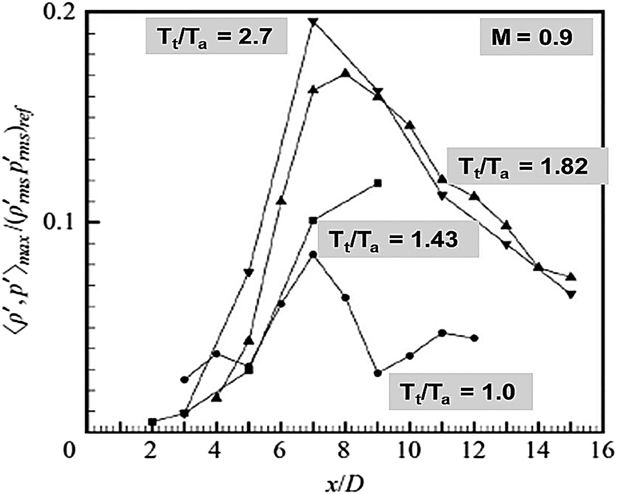

Source distribution measurements with elliptic mirror

The elliptic mirror has the ability to measure noise from both coherent and incoherent sources. This is its biggest advantage, as correlation techniques can sense noise from only coherent sources. Thus, it is a valuable tool when used in conjunction with other approaches. The source measurements were carried out with Boeing’s elliptic mirror, with an aperture of 4.72 ft (1.5 m) and a semi-major axis of 6.73 ft (2.0 m). The principle of the elliptic mirror system is first reviewed. Figure 51 (top) shows a schematic of the elliptic mirror, with a near and far focus. The microphone is located at the near focus and the source of interest at the far focus. For applications to jet noise, the far focus is typically located on the jet centerline. The combined path length (L₁ + L₂) controls the relative phase between the acoustic rays arriving at the microphone via different parts of the mirror. When the source is at the far focus, the combined distance (L₁ + L₂) is constant and the microphone senses a strong signal. However, when the source is displaced transversely (that is along the jet axis) from the major axis of the mirror, the path lengths begin to vary and there is destructive interference, resulting in a drop in the strength of the sensed signal. Thus, the mirror has the desirable property of distinguishing between sources that are located on the far focus from those that are displaced in the transverse or lateral directions. It should be kept in mind though that the resolution is not a sharp point but a small region near the far-focus.

Figure 51.

Top: operating principle of elliptic mirror; Bottom: CAD rendering of mirror and traversing mechanisms in axial and radial directions; jet rig and wind tunnel also shown.

When the source is located on the major axis of the mirror but not at the focus, the response of the mirror is different: the response is insensitive since the variations in the path lengths from different reflection paths from the mirror are much less than for transverse offsets of the source. That is, the mirror does not distinguish between sources that are located along the major axis of the mirror, within a certain range. Therefore, one cannot differentiate between sources located on the near (front) and far (back) shear layers of the jet. This lack of sensitivity in the direction of the mirror major axis is a useful property, in that it allows the mirror to “listen” to an entire slice of the jet. The measurements should therefore be interpreted as the total noise radiated by the axial slice of the jet; the ‘slice of the jet’ approach has been employed for many decades in jet noise theory and is a useful concept for mirror application. The spatial resolution is a strong function of the source frequency; higher frequencies are better resolved since the same difference in the path lengths results in larger phase difference. The reduced resolution of the lower frequency waves is a problem associated with all microphone array techniques as well. The resolution limit at the lower frequency for the mirror is ∼ 1500 Hz. The jet considered here has a Mach number of 1.9. A convergent-divergent nozzle of exit diameter of 1.27 in (3.23 cm) was operated at the design Mach number. A small nozzle diameter was specifically chosen to drive the peak frequencies to higher values, so that the lower frequency limit for the resolution of the elliptic mirror does not affect the measurements at frequencies of interest.

Figure 51 (bottom) shows a CAD drawing of the mirror set-up. The mirror was mounted on a traversing cart that could be precisely positioned at any desired axial location, thereby allowing the mapping of the jet noise sources along the jet centerline. Further, the mirror could be swiveled on its axis and moved along the radial direction (or y-direction) on rails mounted on a platform, attached to a super-structure. This ability to control the mirror position in two directions enables the measurement of the noise radiated from different axial regions of the jet to different polar angles, with a range of view angles from 90° to 150°. It is well known that jet noise exhibits strong directivity. At the lower polar angles and up to ∼90°, (1) the directivity curve is flat; and (2) the spectral characteristics are similar. Therefore, a view angle of 90° for the mirror should be representative of all the lower polar angles. A Bruel and Kjaer Type 4135 quarter-inch microphone was installed at the near focus of the elliptic mirror; narrowband data with a bin spacing of 23.4 Hz were acquired and synthesized to produce 1/3-octave spectra, in the range of center band frequencies of 200 Hz to 80,000 Hz.

A formal theory and the application of the directional microphone system have been explained in depth in Laufer, Schlinker and Kaplan,⁹⁷ Schlinker, Petersen and Kaplan¹²¹ and Chu, Laufer and Kao.¹²² In particular, excellent agreement of the spectra obtained from the summation of the source distribution along the jet centerline with those from an omni-directional microphone located in the farfield was demonstrated; see Figures 6 and 7 in Laufer, Schlinker and Kaplan⁹⁷ for example. A simpler approach has been adopted here, as described in Viswanathan.^92,123 Because of this restriction, the results presented here constitute “apparent source strengths” and should be taken as such. Source distributions have been mapped for a variety of nozzles: unheated and heated subsonic jets from a conic nozzle, supersonic jets from a convergent-divergent nozzle with design Mach number of 1.9, confluent nozzles with internal splitters and lobed mixers, and exposed lobed mixers. Extensive results may be found in Viswanathan.^92,123

Sample results are now presented to highlight the key findings. Figure 52 shows the axial variation of the OASPL per unit length for an unheated M_j = M_d = 1.9 jet, at seven angles. There is strong radiation to aft angles, with the levels dropping rapidly when we go from 140° to 110°. The peak location is identified with a small blue arrow at each angle. The peak locations for the lower radiation angles of 90°–110° is at ∼16D, which is downstream of the end of the potential core. The spectral shapes at the lower angles and up to 110° correspond to the FSS shape. The observed trend suggests that the noise source or the fluctuations in kinetic energy of the fine-scale turbulence is at its highest level there. As discussed in Tam et al.,¹¹³ the direction of radiation of small blobs of turbulence is statistically isotropic. It is, therefore, not surprising that the noise source distribution is insensitive to the direction of radiation. On the other hand, the noise source distribution curves for radiation from 130° to 150° do not peak at the same location; the peak location moves upstream with increase in the radiation angle. This trend is consistent with direct correlation measurements of large turbulence structure noise source for a supersonic jet measured with the Rayleigh-scattering technique, see Figure 29(a) in Tam et al.¹¹³. The reason behind this phenomenon is not known at the present time. Similar trends of two separate noise producing regions for supersonically convective jets were observed by Laufer et al.,⁹⁷ long before the idea of two distinct components had been proposed by Tam.

Figure 52.

Axial variation of the overall source strength radiated to various angles. M = 1.9, T_t/T_a = 1.0.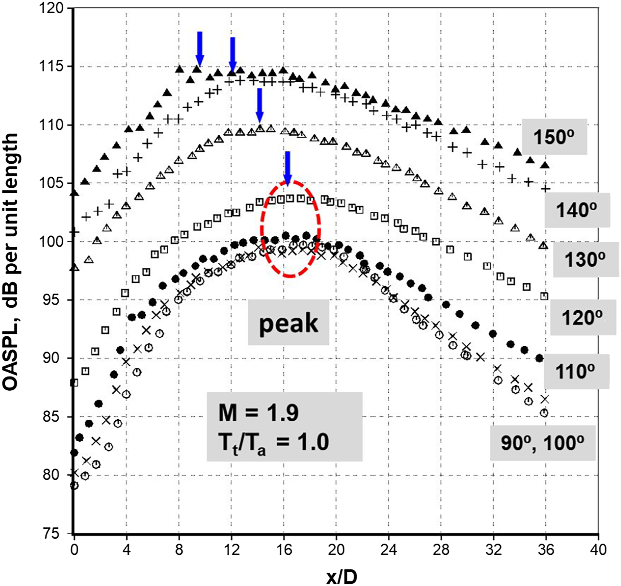

It is instructive to investigate the source distributions for two subsonic jets: M = 0.9, T_t/T_a = 3.2, M_c = 1.05 and M = 0.4, T_t/T_a = 1.0, M_c = 0.28 in Figure 53. For the supersonically convective jet, the peak locations for angles up to 110° occur at ∼8D; at higher angles, they move upstream. These features are similar to those noted for the supersonic jet at a Mach number of 1.9. [Exactly same trends prevail for a M = 1.9, T_t/T_a = 2.2 jet, as shown in Figure 33 in Tam et al.¹¹³]. The peak locations for M_c = 0.28 are very different in Figure 53: they are all clustered at ∼5D for all angles. The spectral shapes at all angles from 90° - ∼130° conform to the FSS shape; further aft, there are differing levels of contributions from the fine scale and large scale turbulence, and the spectral shape is in transition to the LSS shape at 160°. Perhaps it is not surprising then that the peak locations are insensitive to angle.

Figure 53.

Axial variation of the overall source strength radiated to various angles. Top: M = 0.9, T_t/T_a = 3.2; bottom: M = 0.4, T_t/T_a = 1.0.

An examination of the entire database and from other examples shown in Viswanathan⁹² the following features are established: (1) the source of the fine-scale turbulence noise is located downstream of the end of the potential core at all jet velocities; (2) there is no evidence for sources in the initial shear layer, immediately downstream of the nozzle exit plane; (3) the peak locations move progressively upstream with increasing angle for the noise generated by large scale structures; and (4) there is an extended axial region, ∼5D to ∼10D depending on the jet Mach number, where the source strength remains high.

One practical consequence of the results is the following: usually, the noise source is implicitly assumed to be located on the jet axis at the nozzle exit plane in setting up microphones and the subsequent processing of spectra. For this assumption of point source to be valid, the microphone distances must be much longer for supersonic jets so as to ensure that measurements are made in the true geometric and acoustic farfield; see Viswanathan¹²³ for more information.

An interesting question was also addressed in Viswanathan⁹²: what happens to the source locations if we can somehow prevent the formation of a conventional potential core? An exposed lobed mixer was utilized to answer this question. The lobed mixer inhibits the formation of large vortical structures in the flow because of the highly convoluted mixing layer. The mixer sidewalls were scalloped; this geometric feature introduces non-uniformities and adds to the complexity of the flow, thereby destroying any initial circumferential flow symmetry. The source variations for the lower view angles of 90° to 110° for a M = 0.9, T_t/T_a = 3.2, M_c = 1.05 (same as in Figure 53 top) indicate a peak location of ∼1 D_e (D_e is the equivalent diameter of the lobed mixer). For a comparable case for the round nozzle, the peak source location to these radiation angles is ∼ 8D. For larger mirror view angles of 130° to 150°, the peak location is at the nozzle exit.

Finally, the axial distribution of selected frequencies for a jet at M = 1.9, T_t/T_a = 2.2 are displayed in Figure 54 to set the stage for what is to follow in the next section. The radiation angle is 150° and the Strouhal numbers are 0.11, 0.17, and 1.1; the corresponding raw frequencies are 2500 Hz, 4000 Hz, and 25,000 Hz, respectively. Note that these frequencies are higher than the lower resolution limit for the mirror. The peak locations at 150° are at ∼17D for the lower frequencies and ∼10D for a Strouhal number of 1.1. As expected, the peaks for the higher Strouhal numbers move closer to the nozzle exit. Similar trends are observed for other jets. The potential core length for this jet Mach number is ∼ 9D; see Witze¹²⁴. The more pertinent observation is the following: at the lower frequencies, the length of the source region is quite long and spans ∼20D in the axial direction, as denoted by the horizontal blue arrow. That is, the sources for the lower frequencies are definitely not localized but extend over a considerable axial length.

Figure 54.

Axial variation of selected Strouhal numbers at 150°. M = 1.9, T_t/T_a = 2.2.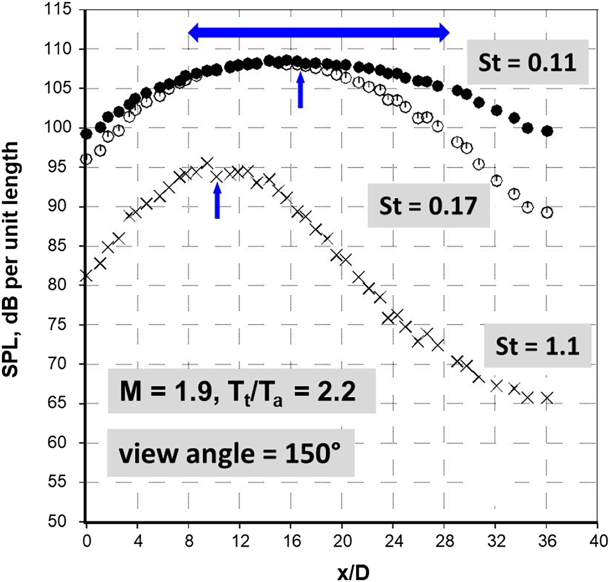

Space-time correlations in nearfield and correlations with farfield spectra

The objective of this investigation is the attainment of better understanding of the physical mechanisms which lead to generation and radiation of noise due to turbulent mixing in jets, through the measurements of nearfield space-time correlations. Implicit in this approach is the assumption that the features of the true sources will be imprinted on the nearfield pressure correlations. Therefore, the interpretations of the results are based on “equivalent” sources. Though the term “source” is used throughout the section, it specifically refers to “equivalent source” and should be taken as such. Space-time correlation characteristics of jets operated over a wide range of jet velocities are examined; correlations of nearfield and farfield spectra provide a wealth of evidence and complement the results already presented. During the collaborative work that resulted in Tam et al.,¹¹³ it became apparent that a key piece of information, space-time correlations in the nearfield, was unavailable at that time. So it was decided to carry out an experimental campaign at LSAF to acquire high-quality data. In a joint effort with Professor Tam, comprehensive plans were made for the data requirements. After a design and manufacture phase, the experiments were carried out in 2009. Complete details may be found in Viswanathan, Underbrink and Brusniak.¹¹² As noted in this paper, advances in flow diagnostic instrumentation and experimental techniques led to a resurgence of interest in gaining a better understanding of the fundamental mechanisms of turbulence-generated noise. A (somewhat) long list of references from the 2000s and the key findings are also included; therefore, they are not repeated here. The use of the measured data in developing and validating a theory for extending the nearfield pressure to farfield spectra are covered in two companion papers, see Tam, Pastouchenko and Viswanathan¹²⁵ and Tam, Viswanathan, Pastouchenko and Tam.¹²⁶

Yu¹²⁷ was perhaps one of the earliest researchers to make measurements in the near acoustic field of high speed jets; this data offered evidence for Mach wave radiation. Troutt and McLaughlin¹²⁸ measured the near acoustic field of a moderate Reynolds number supersonic jet. The near field noise is generated by jet instability waves moving supersonically relative to the ambient speed of sound. The pressure contours from these two studies established the signature pattern of Mach wave radiation, with closed lobe patterns beamed towards large aft angles. Professor Samimy and his students carried out detailed studies of the sound radiated by large scale turbulence, through correlations of pressure in the nearfield and farfield; see Hileman, Thurow and Samimy¹²⁹ and Hileman, Carballo, Thurow and Samimy.¹³⁰

Before we describe the current experiments, attention is drawn to three different studies that used nearfield arrays recently. At NASA Glenn, the hydrodynamic pressure fields of subsonic jets were measured with six circular arrays; see Suzuki and Colonius.¹³¹ The arrays extended to a downstream distance of ∼8D, with a half-cone angle of 11.3°. The radial extent of the microphones was in the range of 1D to 1.75D at x/D = 2.25. Suzuki and Colonius¹³¹ examined the evolution and the modal content of the instability waves in the initial mixing layer and their relation to farfield noise.

A rotating array was used to map the space-time correlations in the nearfield of a transonic and a supersonic jet in the United Technology Research Center (UTRC) experiments, see Reba et al.^132–134. Two linear conical arrays of 8 (or 11) microphones with a half-angle of 7° and an axial spacing of 1.25D were employed; the axial extent of the arrays was 10D (or 14D). The radial distance of the microphones spanned a range of 0.97D closest to the nozzle exit and 2.5D for the most downstream microphone. The pressure fields in this hydrodynamic region are dominated by those associated with the large-scale turbulence structures. They showed that the near-field pressure statistics were well represented by a Gaussian wave-packet model for both the subsonic and supersonic jets.

The studies at the University of Poitiers sought to relate the dynamics of the flow with radiated noise to all radiation angles via the simultaneous measurement of the pressure and velocity fields in the vortical flow, and the pressure fields in the nearfield and farfield; see Tinney et al.,¹³⁵ George, Wänström, and Jordan,¹³⁶ Laurendau et al.,¹³⁷ Guitton et al.,¹³⁸ among others. Through a filtering of the near pressure field and stochastic analysis of the measured parameters, certain relations between the flow characteristics and the farfield spectra were formulated. They employed a linear array with a half-cone angle of 9° and an axial extent of 11D. The axial spacing was 0.2D closer to the nozzle exit and 0.4D further downstream; the radial distance was 0.8D at the nozzle exit plane. A wave number analysis was employed to delineate the hydrodynamic field from the acoustic field.

In the Boeing test, a nearfield conical cage array with a half-angle of the cone of 10° is deployed. There are 21 semi-circular rings, with 14 microphones at various azimuthal angles in each ring, for a total of 294 near field microphones. Figure 55 shows a photograph of the cage array, viewed from the downstream direction; the cascaded rings of microphone diaphragms forming a conical surface are highlighted in this view. The microphones are concentric with the jet axis in this array location. The desire to measure the nearfield and farfield pressures simultaneously dictated the choice of semi-circular rings; this arrangement, with the farfield array located on the opposite side of the nearfield array, allowed a direct line of sight to the farfield microphones by not blocking the acoustic ray path. The following convention is used for defining the azimuthal angles (ϕ): 0° corresponds to the bottom dead center (towards the ground) and the angle is measured counterclockwise. Each azimuthal ring spans 180°, from 180° to 360° (or 0°). The azimuthal spacing is as follows; for the sake of easy comprehension, the azimuthal positions are given with the angles measured in the clockwise direction (there should be no confusion as these angles are obtained by subtracting from 360°), starting from the bottom dead center: 0, 5, 10, 15, 25, 35, 45, 60, 75, 90, 110, 130, 150, and 180°. As seen, the azimuthal spacing starts at 5° initially and incrementally increases to 10°, 15°, 20° and finally to 30° between the last two microphones. The axial spacing between the rings is uniform and is 1.5D for this particular test. Source distribution measurements with the elliptic mirror (Figures 52 and 54) provide critical information as to the requirements of the array length: the axial extent of the array, the distance between the first and the last rings, is chosen to be 30D (6.125 ft in length), based on the length of the low frequency source observed in Figure 54.

Figure 55.

Photograph of the cage array taken from downstream direction. The microphones are concentric with the jet axis.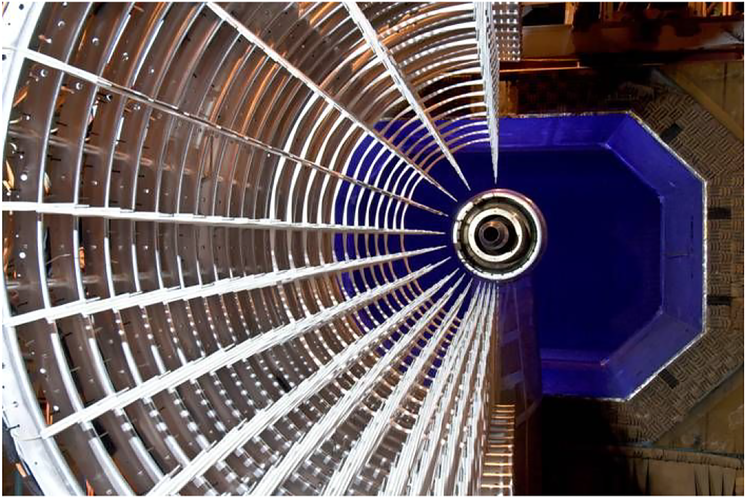

Four different farfield microphone arrays are deployed; these are at azimuthal angles of 90°, 60°, 30°, and 5°, respectively. These four arrays are on the opposite side of the jet from the cage array (which subtends azimuthal angles from 180° to 360°). There are 14 microphones at polar angles of 50, 60, 70, 80, 90, 100, 110, 120, 125, 130, 135, 140, 145 and 150° for the arrays at azimuthal angles of 90°, 60°, and 30°. There are 48 microphones in the farfield, in addition to the 294 on the cage array, for a total of 342 microphones. Once the height of the array is fixed at the proper position (z-direction), the entire array can be moved in the x-y plane. The radial distance of the microphones to the jet axis can be controlled by moving the array in the axial direction. The array can be moved in the lateral direction (y-direction) so as to map the pressure field on a cross-sectional plane, using the microphones located at an azimuthal angle of 270°. The array could also be stowed, farther away from the jet. Electronics and instrumentation were custom-built by Boeing and proprietary software were used to acquire, process and analyze simultaneously sampled space-time data; see Viswanathan, Underbrink and Brusniak.¹¹²

A convergent nozzle and a convergent-divergent (CD) nozzle with a design Mach number of 1.67 are used. Both of them had the same exit diameter of 2.45″, so as to maintain consistency in spacing, etc. for the cage array. Unheated jets and heated jets at a stagnation temperature ratio (T_t/T_a) of 3.2 over a wide range of jet Mach numbers from 0.51 to 1.67 have been considered. The convective Mach number (M_c), taken to be (0.7*V_j/a), spans a range of 0.36 to 1.69. At each jet condition, both nearfield and farfield measurements were made simultaneously at several array positions as follows: (1) the radial distance at the nozzle exit plane (x/D = 0.0) for the conical surface formed by the diaphragms of the cage microphones is 3D from the jet centerline. The cage array spanned a distance of 1D to 31D; (2) the radial distance at (x/D = 0.0) is 3.53D from the jet centerline and the cage array spanned a distance of -2D to 28D; and (3) the radial distance at (x/D = 0.0) is 4.06D from the jet centerline and the cage array spanned a distance of -5D to 25D. Thus, near pressure fields were acquired on three different conical surfaces surrounding the jet, from 3D to 4.06D at the nozzle exit plane. Note that the microphones on the cage array are concentric around the jet axis for these three configurations. In addition, the entire pressure field was mapped on a plane at an azimuthal angle of 270°, at various radial distances at (x/D = 0.0) of 2D, 3D, 4D, 5D, 6D, 7D, 8D, 9D, 10D, 12D, 14D, 16D, 18D and 20D. For these measurements of the pressure field mappings, the axial extent of the array was from the nozzle exit plane 0D to 30D. Pressure signals from all the microphones were recorded for these 14 array positions, even though the locations of the microphones for azimuthal angles other than 270° are not on the plane of interest.

There are critical differences between the current measurements and those of the NASA Glenn, UTRC and Poitiers experiments. Whereas the arrays were in the hydrodynamic field in those experiments, the microphones in the current test are located predominantly in the acoustic field and possibly beyond the influence associated with the decaying instability waves on the nearfield pressure. A more crucial difference is the following: the axial extents of the arrays in these studies are 8D, 10D (or 14D), and 11D, respectively. As will be shown with new results, there is a significant shortcoming with these shorter arrays.

Nearfield space-time characteristics

Extensive data on correlations and coherence for all the jet conditions are presented in Viswanathan, Underbrink and Brusniak.¹¹² Coherence contour maps that capture the global variations for all the cage microphones, at various convective Mach numbers, are included in this reference; these are not repeated here. Sample time-domain results that highlight the main findings are reproduced here. Figure 56 shows the correlation functions, with the fixed reference microphone at ϕ = 0° (bottom dead center) and x/D = 20.5 and the second microphone at ϕ = 0° and x/D over a range of 13.0 to 31.0. The cage array position is at r/D = 3.0 at x/D = 0.0. Three different jet conditions are considered: (top): M_j = 1.67, T_t/T_a = 1.0; (middle): M_j = 0.9, T_t/T_a = 3.2; (bottom): M_j = 0.51, T_t/T_a = 1.0. The trends are very similar for all jet velocities. The maximum correlation level is ≥ 0.4 (or 40%) for the entire range of axial distance, with significantly higher correlations of ≥ ∼0.6 from x/D = 16.0 to 31.0. It is incredible that this high level of correlation exists for an extended axial region of ∼18D.

Figure 56.

Axial correlation, reference microphone at ϕ = 0° and x/D = 20.5; r/D = 3.0 at x/D = 0.0. Second microphone at ϕ = 0° and x/D = 13.0 to 31.0. (top): M_j = 1.67, T_t/T_a = 1.0; (middle): M_j = 0.9, T_t/T_a = 3.2; (bottom): M_j = 0.51, T_t/T_a = 1.0.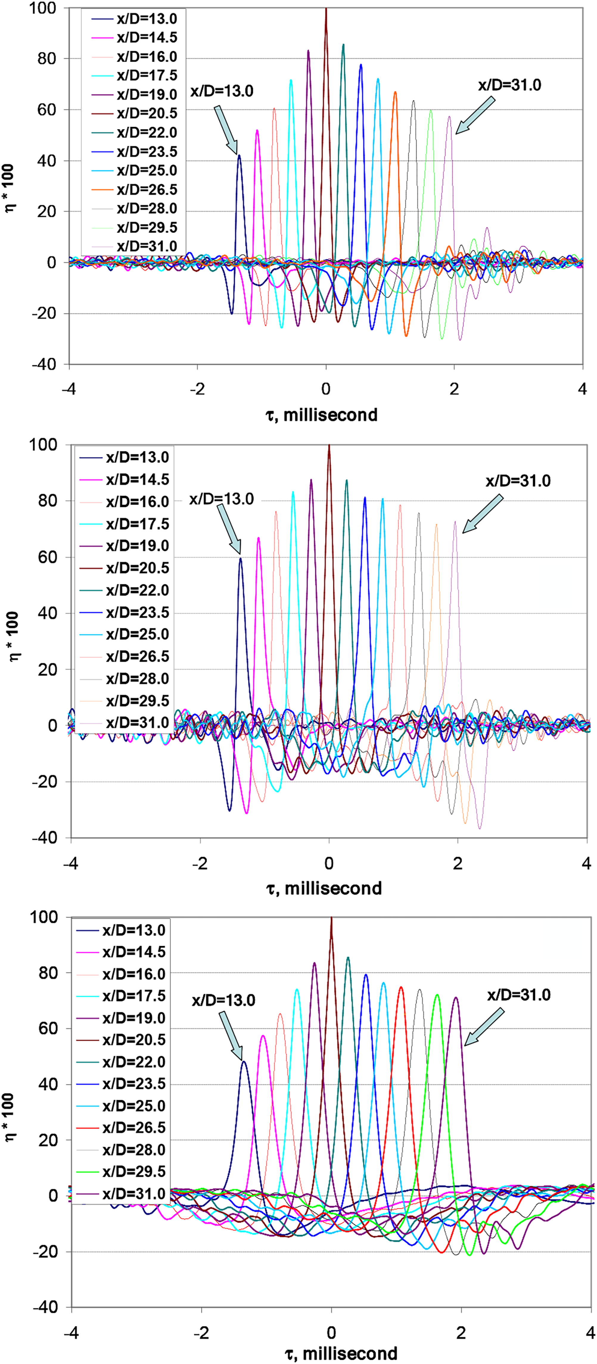

In the coherence contour maps [Figures 16–19, with M_j = 1.67, T_t/T_a = 3.2; M_j = 0.51, T_t/T_a = 1.0; M_j = 0.51, T_t/T_a = 3.2; and M_j = 0.9, T_t/T_a = 3.2; respectively, in Viswanathan, Underbrink and Brusniak¹¹²] the effect of the location of the reference microphone was investigated as follows: the maps were produced at six x/D locations of 4.0, 10.0, 16.0, 20.5, 25.0 and 29.5. There is very little coherence when the reference microphone is located at x/D = 4.0, even in the azimuthal direction between microphones in the same ring. In general, no coherence is detected from the nozzle exit plane to ∼7D downstream for all jet conditions; this trend suggests that only random turbulence fluctuations are present in this region. At x/D = 10, a definitive trend starts to emerge with good correlations over a few diameters, indicating that the flow structures are beginning to get organized. At x/D = 13, there is high correlation all around the periphery of the jet covering 360°, see Figure 12 in Viswanathan, Underbrink and Brusniak.¹¹² When the reference microphone is at x/D≥16, dramatic changes in the contour maps are observed. The axial extent of regions of high coherence, arbitrarily taken to be ≥ 0.5, is ∼ 15D; this large source is coherent all around the periphery of the jet (360°). [For correlations ≥0.4, the axial extent is ∼ 18D]. The high coherence levels are generally confined to the lower frequencies. Let us reinforce this finding: a very high value of correlation/coherence (50%) prevails for any single position at any axial location, with every other position in a region with an axial extent of ∼15D for all jet velocities. This is indeed quite remarkable. Exactly similar trends are observed when the array location is moved radially such that r/D = 2.0 and 4.06, at x/D = 0.0, respectively.

One more observation needs to be clarified. The time-domain correlations have been normalized by the autocorrelations with zero time delay for that particular jet Mach number and temperature ratio. It is instructive to examine the axial variations of the maximum autocorrelation (unnormalized or normalized by unity) levels at different jet conditions. Such a variation is shown in Figure 57 for six jet conditions: M_j = 0.51, 0.9 and 1.67, at two temperature ratios of T_t/T_a = 1.0 and 3.2. There is the expected increase in level with increasing jet velocity, as the higher velocity jet radiates higher levels of noise to the farfield. The maximum levels are comparable for the unheated supersonic jet (M_c = 0.93) and the heated subsonic jet (M_c = 1.05) because the convective Mach numbers are not dissimilar. The trends over the entire axial distance are similar for the two subsonic jets with comparable convective Mach numbers of 0.58 (M_j = 0.9 and T_t/T_a = 1.0) and 0.64 (M_j = 0.51 and T_t/T_a = 3.2). The peak locations for maximum pressure occur between ∼6D – ∼8D for all the jets; thus, the peak locations are observed near the end of the potential cores for all the jets. However, the peak coherent source is located from ∼13D to ∼31D as seen in Figure 56, and highlighted by the shaded rectangle in Figure 57. That is, the strong coherent source is located well beyond two potential core lengths from the nozzle exit. This is a notable new finding and is contrary to existing belief. It is also worth pointing out, that this large coherent source was completely missed in the prior investigations with nearfield arrays because of the shorter axial extents of the arrays.

Figure 57.

Axial variation of maximum autocorrelation at each x/D. M_j = 0.51, 0.9, and 1.67; T_t/T_a = 1.0 and 3.2. Peak locations highlighted by arrow at x/D = ∼7. Location of large coherent source, from x/D of ∼13 to 31, highlighted by shaded rectangle.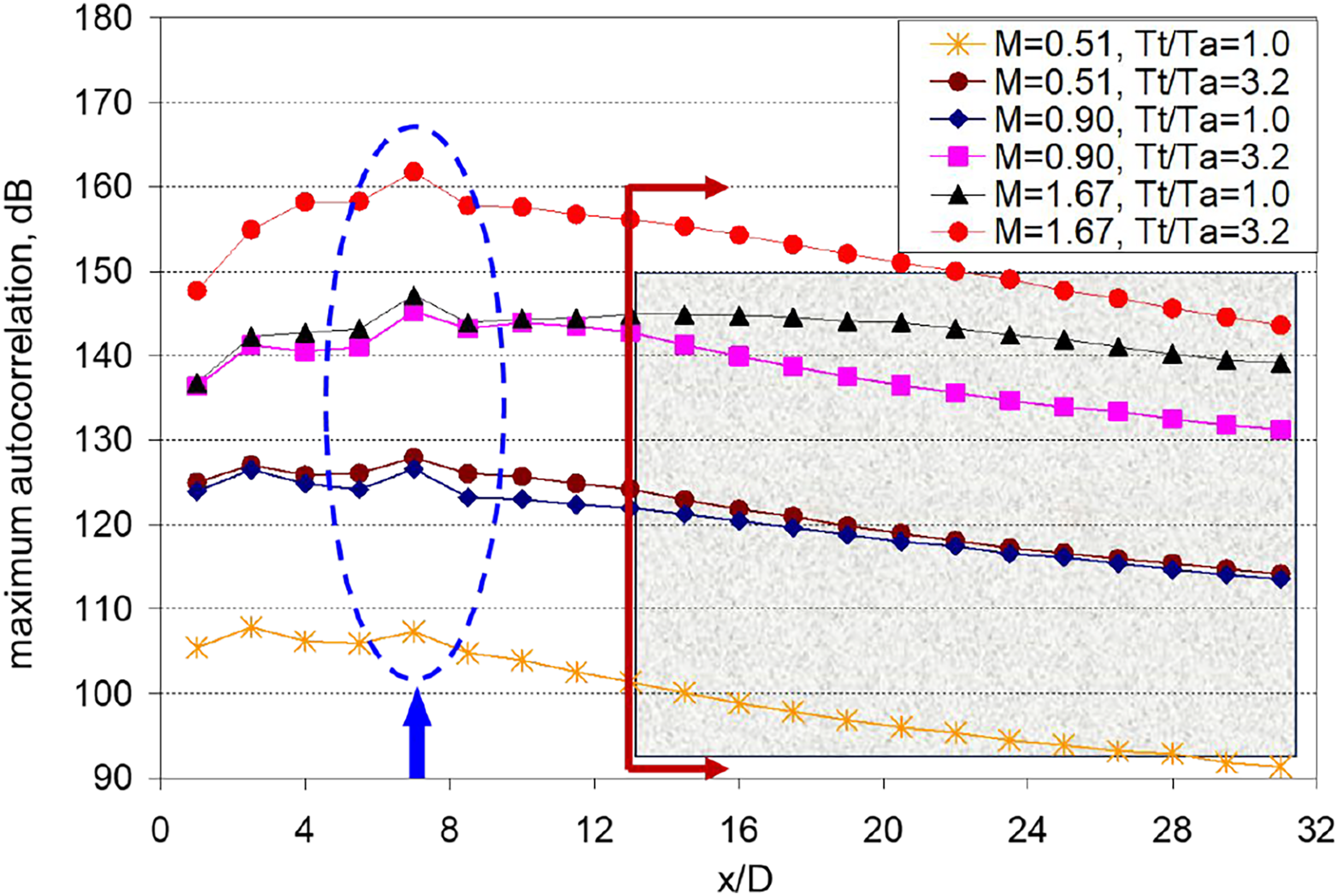

Nearfield-farfield correlations

The nearfield cage array indicates an axisymmetric sound field, with high correlations over 360°; the same feature is detected by the azimuthal array in the farfield. In the nearfield-farfield correlations below, the reference cage microphones are at an azimuthal angle of 0°, while the farfield microphones are at an azimuthal angle of 90°. That is, there is an azimuthal separation of 90°. An overall picture of the noise radiation from different portions of the jet to particular radiation angles is obtained when the axial variations of the maximum correlation levels with angle are examined. The effect of heating the jet from T_t/T_a = 1.0 to 3.2 at three different Mach numbers of 1.67, 0.9 and 0.51 are investigated in this fashion. The supersonic jet is first considered in Figure 58. There is close to zero correlation with all the angles when the nearfield point is located at x/D ≤ ∼7 for the unheated jet. Further, the correlation levels are <0.1 (10%) for radiation angles <130°, for all the nearfield locations. The peak levels start to increase dramatically with x/D as the radiation angle is increased: a maximum level of ∼0.65 is reached for the microphone at 150°. The observed trends for the heated supersonic jet are markedly different: (1) there is a measurable level of correlation for the lower radiation angles of 120° to 130°, with the maximum level of ∼0.33 for 130°; (2) the peaks for the lower angles occur at distances that are closer to the nozzle exit; (3) there is a well-defined progression of peak axial distance from the nozzle exit plane with increasing radiation angle from 120° to 140°; (4) there is virtually no correlation for 110° even for this highly heated jet; and (5) there is also a rapid decay in the correlation levels with downstream distance beyond the peak location, for the lower polar angles.

Figure 58.

Peak nearfield-farfield correlations. Reference microphone at all x/D and ϕ = 0°. Farfield microphones at 120° to 150°. (a): M_j = 1.67, T_t/T_a = 1.0; (b): M_j = 1.67, T_t/T_a = 3.2.

The high subsonic jet with M_j = 0.9 is considered next in Figure 59. As in the unheated supersonic jet, the correlation levels are low and of the order of < ∼0.1 (10%) for radiation angles <130°. High peak correlations are observed at large aft angles, with a value of ∼0.65 at 150°. The characteristics for the heated jets are again different from those for the unheated jet: measurable correlation levels are observed for 120° to 130° and the distance of the peak axial location from the nozzle exit increases with increasing radiation angle. Though there are similarities between the trends for the M_j = 0.9 and 1.67 jets at T_t/T_a = 3.2, there is also a big difference: for the M_j = 1.67 jet, there is a slower initial growth for the peak values and a longer initial region of low correlations, which increases monotonically with increasing radiation angle; for the M_j = 0.9 jet, the peak values start rising immediately from x/D = ∼5 and the peak correlation levels are reached by x/D = 13 for all the angles.

Figure 59.

Peak nearfield-farfield correlations. Reference microphone at all x/D and ϕ = 0°. Farfield microphones at 120° to 150°. (a): M_j = 0.9, T_t/T_a = 1.0; (b): M_j = 0.9, T_t/T_a = 3.2.

Finally, the low subsonic jet with M_j = 0.51 is investigated in Figure 60. Similar to the characteristics for the higher Mach numbers, the trends are different for the heated and unheated jets. The pattern of noticeable correlation in the angular range of 120° to 130° is once again observed for the heated jet. Furthermore, there is a gradual decay of the correlation following a rapid growth at these lower angles for the heated jet. Peak correlation levels of ∼0.8 (80%) are observed over an extended axial distance, from x/D = 13 to x/D = 31, for large aft angles ≥145°. The peak correlation levels for all the jets at an angle of 150° ranges from ∼0.48 to ∼0.83. The lowest peak correlation level occurs for the heated M_j = 1.67 and the highest level for the heated M_j = 0.51 jet. One should not misinterpret these raw numbers as implying that the lower Mach number jet has higher source strength for the following reason: these are normalized correlation levels. The autocorrelation levels change with x/D and jet conditions, as shown in Figure 57 (which in a sense is normalized by a reference value of unity). The fundamental conclusions from these plots are: (1) there is a large coherent source region that predominantly radiates to the aft angles for jets at all convection Mach numbers, from 0.36 to 1.69, and (2) this source is located from ∼13D – ∼31D, which is well beyond the end of the potential core. In this regard, the noise radiation mechanism responsible for large aft angles seems to be the same regardless of jet velocity. This point will be further reinforced in the following sections.

Figure 60.

Peak nearfield-farfield correlations. Reference microphone at all x/D and ϕ = 0°. Farfield microphones at 120° to 150°. (a): M_j = 0.51, T_t/T_a = 1.0; (b): M_j = 0.51, T_t/T_a = 3.2.

The reason for the noticeable correlation in the angular range of 120° to 130° for the heated jets can be gleaned through an examination of the spectral shapes in Figure 2. At the lower polar angles of 90° and110°, the spectral peaks are broad and conform to the shapes of the fine-scale similarity spectrum. At an angle of 120°, the spectral shape changes and there is some contribution from the large scale structures; at this angle, there is contribution from both sources, as highlighted by the arrow and the slanted lines. As the radiation angle increases, the contributions from the large scale turbulence become progressively more dominant and the spectrum finally conforms to that of the large similarity spectrum at 150°. Note that the spectral peak is narrow. It was shown earlier from farfield correlation measurements that there is virtually no correlation when the spectral shape conforms to the fine-scale similarity shape and there is significant correlation when the spectral shape conforms to the large-scale similarity shape. For the unheated jet, the spectra up to 130° are characterized by the fine-scale similarity shape. Perhaps it should not be surprising then that there are noticeable nearfield-farfield correlations, because of the contributions from the coherent structures in the angular range of 120° to 130° for these highly heated jets with T_t/T_a = 3.2.

In summary, the source distribution measured with the elliptic mirror indicates a large source region, especially for the low frequencies from ∼10D to ∼30D. The large coherent region, from ∼13D to ∼31D, observed in the nearfield is concentrated at low frequencies as well. That is, there is a precise overlap of these two regions. The nearfield-farfield correlations indicate high levels from any single location in this large source region with spectra in the aft angles ≥135° for all jet velocities.

Results from the nearfield mapping from 3D to 20D are presented in Viswanathan, Underbrink and Brusniak.¹¹² There are well-defined closed lobes pointed in the downstream direction, very similar to the measurements of Troutt and McLaughlin.¹²⁸ The significance of these loops, as being due to the growth, saturation and decay of instability waves, is explained by Tam.¹³⁹ Tam^31,139 showed that the nearfield pattern of a high-speed jet obtained with an instability wave analysis closely matches the measured contours by Troutt and McLaughlin.¹²⁸

In the two-part analytical work of Tam, Pastouchenko and Viswanathan¹²⁵ and Tam, Viswanathan, Pastouchenko and Tam,¹²⁶ the problem of extending the near acoustic field of a high-speed jet to the far field is considered. Unlike past practices that employ Kirchoff methods or surface Green’s function, an adjoint Green’s function is used. One significant advantage of using the adjoint Green’s function is that for a given direction of radiation, one is required to solve only a single acoustic scattering problem. For problems involving a broadband time-stationary sound field such as the noise field of a high-speed jet, it is shown that the two-point space-time pressure correlation function on the bounding surface is the equivalent noise source. By using a conical surface placed sufficiently close to the jet flow, it is believed that the noise source characteristics are imprinted on the two-point space-time pressure correlation function. Thus it becomes possible to study the noise source location, intensity, frequency distribution and other characteristics by using near field measurements. Because the present method requires measuring only the fluctuation pressure on the bounding surface, it has a definite advantage when it is used to extend an experimentally measured near acoustic field to the far field. Commonly used methods such as the Kirchhoff integral method or the Ffowcs-Williams and Hawkings equation require measuring three or more variables, which would well-nigh be impossible. Validation tests are provided in the first part.

In the second paper, the proposed method is applied to the supersonic jet, with M_j = 1.67 and T_t/T_a = 3.2. The measured data are utilized for two purposes. The first objective is to validate the near field to far field continuation method developed in the Part I paper. The second, but more crucial, objective is to obtain a new understanding of the characteristics of the sources of high-speed jet noise. Figure 61 (top) shows a comparison between the measured spectrum at 130° with that obtained with the continuation from the nearfield correlations. Figure 61 (bottom) depicts a comparison between the directivity of the measured Strouhal number of 0.26 with that calculated by the continuation method. The good agreements not only validate the continuation method but also provide support in identifying the two-point space-time pressure correlation function as the equivalent noise source of the jet. This is significant: the noise source characteristics of the jet can consequently be studied by examining and analyzing the characteristics of the equivalent noise source measured on the conical surface without making measurements inside the turbulent jet. At this juncture, it is useful to point out that even if it is feasible to make measurements inside the jet flow, it is not obvious what parameter that would define the noise source should be measured.

Figure 61.

Top: comparison of measured spectra with continued from nearfield correlation data. Bottom: comparison of farfield directivity at Strouhal number of 0.26. open symbols: data, closed symbols: continued from nearfield. M = 1.67, and T_t/T_a = 3.2.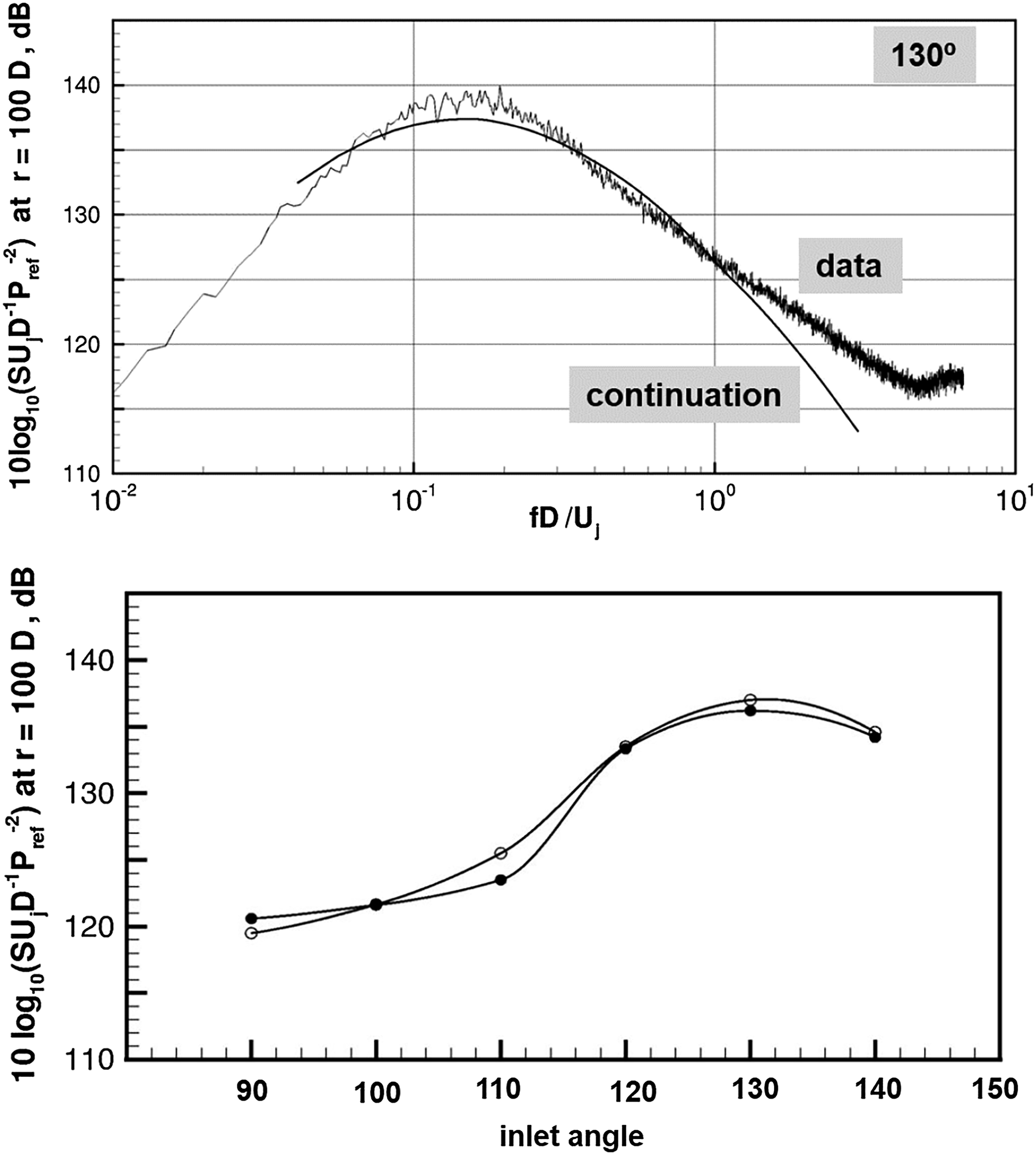

A wealth of information is provided in the above three papers related to the cage array measurements, theoretical development and analyses (especially in the first and third papers). All measured data indicate that the noise source near the jet nozzle exit is highly random and small in size. The noise source becomes more and more organized, and increases in size in the downstream direction. Beyond the potential core of the jet, the noise source is quite axisymmetric and coherent over a distance of many jet diameters. The experimental evidence points to the fact that near the nozzle exit the dominant noise source is the small scale turbulence of the jet flow. Farther downstream, the dominant noise source is the large turbulence structures.

The noise source of high-speed jets may be decomposed into azimuthal modes. This is done in the third paper to provide a different perspective of the characteristic features of the noise source. It is found that the most intense noise source component is associated with the axisymmetric mode. Contributions to the radiated noise from modes higher than the second mode are negligible. The peak intensity is located more than two potential core lengths downstream. Single point pressure fluctuations in the near field of the jet is found to peak near the end of the potential core, as seen in Figure 57. It is, therefore, believed that single point statistics are not appropriate indicators of noise source location and strength of large scale turbulence. By means of the measured cross-spectrum function of the equivalent noise source, strong evidence of the jet noise source containing a significant wave component is provided. This is another clear indication that the large turbulence structures of the jet flow constitute a dominant noise source.

To summarize, a variety of evidence has been adduced using five different approaches. The salient observations are mutually supporting, and the cumulative weight lends credence to the proposition that there are two distinct sources of turbulent mixing noise.

Shock-associated noise

The phenomenon of broadband shock-associated noise was first identified as a significant noise component for imperfectly expanded supersonic jets by Harper-Bourne and Fisher.¹⁴⁰ This component is rich in spectral detail. Since their pioneering work, there have been several investigations of shock-associated noise, a few of which may be found in: Tanna,¹⁴¹ Seiner and Norum,^142,143 Norum and Seiner,^144,145 Tam and Tanna,¹⁴⁶ Seiner,¹⁴⁷ Seiner and Yu,¹⁴⁸ Norum and Shearin¹⁴⁹ and Yamamoto et al.¹⁵⁰.

In the theoretical arena, seminal research has been carried out by Professor Tam; though it sounds implausible, his contributions to the physics of broadband shock-associated noise and screech tones perhaps surpass his output on turbulent mixing noise! As per his theory, the broadband component is generated by the weak but coherent interaction between the large-scale turbulent structures in the jet shear layer and the quasi-periodic shock cell system. Formulae for the peak frequency and intensity were also developed. A prediction method based on this theory was able to reproduce the observed characteristics very well. A brief list of his references may be found in: Tam,^151–154 Tam, Jackson and Seiner,¹⁵⁵ Tam, Seiner and Yu,¹⁵⁶ Tam, Ahuja and Jones,¹⁵⁷ among many others. It is not possible to highlight the significant results, interpretations, and explanations reported in all these references here. For a comprehensive treatment of this topic, see Tam³¹ and the references therein. Raman^158,159 provides an extensive list of references on screech tones.

A single example of broadband shock-noise spectra and comparison with turbulent mixing noise measured by Norum and Seiner,¹⁴⁵ is reproduced here from Tam³¹ as Figure 62. The jet conditions are M = 1.49, T_t/T_a = 1.0, and M = 1.67, T_t/T_a = 1.0. The nozzle design Mach number M_d = 1.5. The magnitude of the shock-noise above the mixing noise is clearly evident at all angles. The main characteristics of broadband shock noise as noted by Tam are the following. Each noise spectrum is dominated by a single peak; a small second peak is also observed at 75° and 90°. The frequency at the peak increases with increasing angle. The maximum level at the shock peak is also indicated at each angle, which decreases from 117.3 dB at 30° to 100.5 dB at 120°. As mentioned by Tam, the fact that the peak frequency is a strong function of the angle suggests that noise radiation is coherent and directional and that it is from a coherent source. Another characteristic of the shock component is that the half-width of the spectral peak increases with inlet angle. A strong screech tone at a fixed frequency at all the angles can also be observed at the lower angles. The fundamental screech tone frequency is always smaller than the frequency range of the broadband component and is a reliable indicator of the lower limit of the broadband shock noise. This figure encapsulates the characteristics of all three components of noise.

Figure 62.

Noise spectra of single-stream jet measured by Norum and Seiner¹⁴⁵ Fully expanded M = 1.49 and M = 1.67. T_t/T_a = 1.0. Nozzle design Mach number M_d = 1.5. Reproduced from Tam.³¹

Viswanathan⁷² demonstrated that the scaling law could be used to separate the shock-associated noise from the mixing noise, by subtracting the scaled mixing noise from the measured total. There are additional issues associated with extending the scaling law from subsonic to supersonic jets. The phenomenon of nonlinear propagation is a concern at aft angles, as seen in Figures 30–32. Good spectral collapse is obtained only at the lower frequencies, to the left of the spectral peak. Further, the peak directivity moves to a lower angle for highly heated supersonic jets. However, these concerns are not too pertinent at lower angles, where separation is required. From an examination of the entire supersonic and subsonic database it has been determined that the scaled mixing noise is typically within ∼1 dB to ∼ 2B (if screech tones are present) of the measured total at the lower frequencies, where the mixing component is dominant. In practice, the scaled mixing noise spectrum is moved up by ∼ 1 dB to match the data. It is possible now with this procedure to assess the relative importance of the two components for various jet operating conditions.

Figure 63 shows the directivities of the overall sound pressure levels of the two components for an M_j = 1.36 jet at three temperature ratios of 1.0, 1.8 and 3.2, obtained with a convergent nozzle. For the unheated jet, the shock component is clearly dominant at the lower polar angles, with the levels being higher by ∼ 15 dB. In the aft directions, the mixing noise is dominant. As the jet is progressively heated, the mixing noise levels increase monotonically and the difference in levels between the shock and mixing components decrease. However, there is only a minor effect of temperature on shock noise, which quickly becomes negligible when the jet stagnation temperature is increased to 1.8; see Viswanathan et al.⁸⁰. At the highest temperature ratio of 3.2, the shock noise is only ∼5 dB higher than the mixing noise at angles ≤ 80°. Beyond 120°, the mixing noise levels are substantially higher. Another notable feature in the directivity of the shock component is the following: the overall levels vary only slightly with radiation angle. Though the peak value decreases with inlet angle in Figure 62, the spectral half-width increases with angle, thereby offsetting the peak level reduction. The slightly elevated levels at some angles for the lower temperature jets (T_t/T_a = 1.0 and 1.8) are caused by screech tones; these have not been removed in the calculation of the OASPL.

Figure 63.

Directivity of the mixing and shock components at different temperature ratios. Mj = 1.36. ▲: shock noise; ●: mixing noise.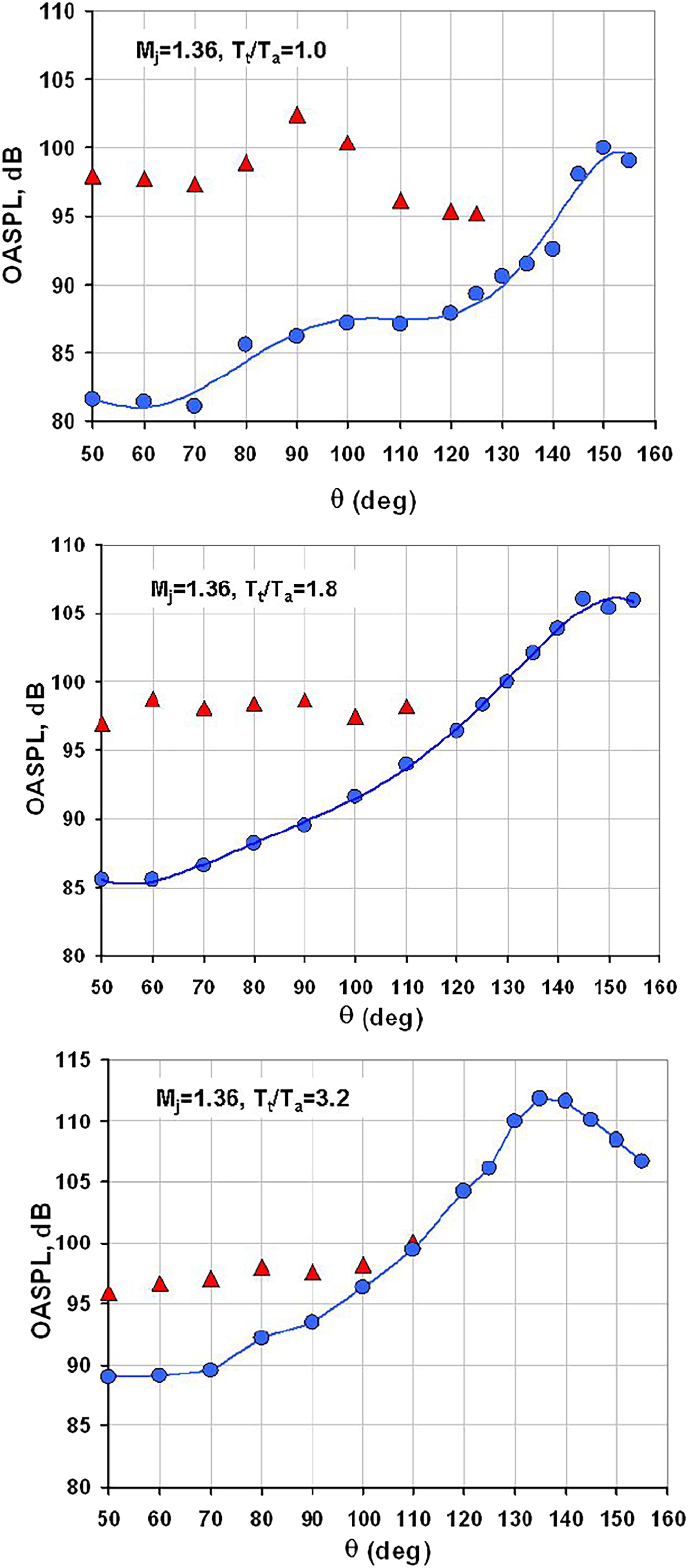

It is worth remembering that shocks are present only for engines that power fighter aircraft, which are operated at off-design conditions during takeoff. These engines have convergent-divergent nozzles with straight divergent sections, wherein weak shocks are always generated. The stagnation temperature ratio usually exceeds 3.0. The shock intensity which can be approximately estimated to be [M_j ² – M_d ²] ² is ∼ 0.46 for typical MIL power, see Figure 1. The shock intensity in the above example in Figure 63 is ∼ 0.72. Therefore, the turbulent mixing noise is a lot stronger than shock-associated noise for fighter aircraft, a point emphasized with Figure 1. There are no community noise restrictions for fighter aircraft. However, military personnel are positioned close to the aircraft on aircraft carrier decks. Even if one is positioned in front of the plane, that person will be blasted by the high mixing noise when the aircraft starts rolling forward and takes off. Solutions must be found to mitigate turbulent mixing noise.

Practical applications

So far, the focus has been on understanding the spectral characteristics both statically and in the presence of a flight stream, as well as the nature of the sources of turbulent mixing noise for single-stream jets. Now we are concerned with real-world airplane applications, with the objective of assessing noise from commercial engines/aircraft and noise certification. Perforce, any method should be simple, easy to use and not require long computing times. As already mentioned, all commercial engines are operated at subsonic Mach numbers even at maximum takeoff power. The bypass ratio (BPR) of modern turbofan engines has been rising steadily over the last four decades and has reached ∼10 at takeoff power. Further, the nozzle pressure ratio (NPR) has been dropping steadily. The SAE method (1994) was originally developed by Lu¹⁶⁰ at Boeing, and was revised subsequently. As stated by Lu, the validity of the method is restricted to a maximum BPR of ∼5.5. The BPR of earlier generation turbofan engines is typically ≤ ∼5. There have been several attempts, but mostly unsuccessful, to update this method. Significant discrepancies between the SAE predictions and measured data have been noted by many engineers.

Comparison of model-scale spectra with engine spectra

First, it needs to be established that the knowledge gained from scale model investigations and the results therein translate to jet engines. A careful experimental study has been carried out to verify whether a model-scale nozzle produces the same jet noise as a jet engine, with the twin goals of (1) validating the practice of carrying out jet noise research at model scale for full-scale applications, and (2) aiding the identification of jet noise in measured total spectra from jet engines, which have contributions from several noise sources. Viswanathan⁷⁹ examined the various issues that must be considered and resolved when comparing the two sets of data; these are not repeated here. A special test was carried out with a turbojet engine (with some cooling, which results in a very low bypass ratio), so as to minimize the contributions from the turbomachinery sources. Several measures, which turned out to be highly successful, were taken to measure pure jet noise. A sample spectral comparison between extrapolated model data and engine data are displayed in Figure 64. Spectra at two different power settings, one subsonic and one supersonic, are shown at four angles of 70°, 90°,130°, and 140°. The symbols denote engine data and the lines denote model scale data. There is excellent agreement between the two sets of spectra at all the angles. Similar comparisons at other angles and other engine power settings may be found in Viswanathan.⁷⁹ It is clear that model scale jets indeed generate the same jet noise as a turbojet engine, provided a variety of steps are taken and care is exercised in each test. Our interest is in modern high bypass ratio turbofan engines, which is addressed in the next section.

Figure 64.

Comparison of model scale spectra and engine spectra at two power settings for turbojet engine. Symbols: engine data; lines: model data.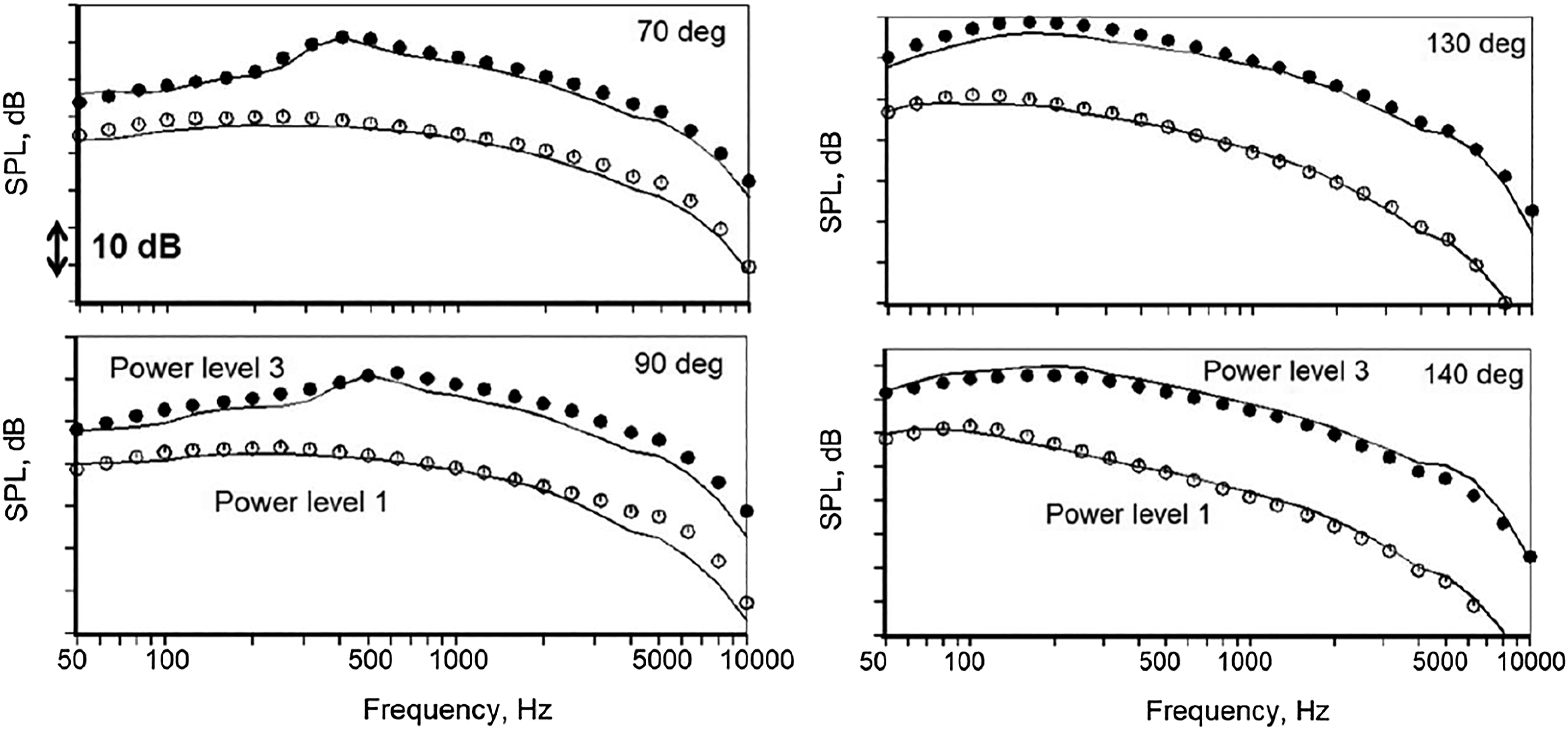

New method for spectral prediction of jet noise from turbofan engines

The scaling law for single-stream jets described here provides a fresh avenue for developing a brand new spectral prediction method. The prediction method must be applicable and accurate over a very wide range of BPR, from lower bypass ratios (∼4) to ultra-high bypass ratios (∼20), to cater to any future engine. Central to this effort is the generation of a database at high BPR that would permit the quantification of changes to the spectra at all angles, when the engine cycle conditions are changed. A comprehensive database was acquired, as described in Viswanathan¹⁶¹ and Viswanathan, Czech and Lee.¹⁶²

The exhaust of a turbofan engine is characterized by a host of parameters: primary nozzle pressure ratio (NPR_p), primary stagnation temperature (T_p), secondary nozzle pressure ratio (NPR_s), secondary stagnation temperature (T_s), secondary-to-primary jet velocity ratio (V_s/V_p), and secondary-to-primary nozzle area ratio (A_s/A_p). The subscripts ‘p’ and ‘s’ denote primary (core) and secondary (fan) streams, respectively. The noise from a dual-stream nozzle is dependent on the above thermodynamic and geometric parameters, which characterize the noise sources regions. It is worth remembering that the geometric area ratio is fixed for a given engine, whereas the thermodynamic parameters vary as a function of engine power setting, denoted by the shaft rotational speed N1. Therefore, it is more meaningful to focus on the area ratio (A_s/A_p) rather than the BPR, as the BPR is highly dependent on the engine power setting. Further, the cycle conditions in the primary (core) and secondary (fan) streams are not too dissimilar for different engines. The area ratio of the older turbofan engines is typically ≤∼3.0. There was a steep increase in area ratio to ∼4.8 for the GE90 engine; the BPR at takeoff increased to ∼8.0. The area ratios for the newer engines typically span a range of ∼4.0 to ∼5.2. The range of Strouhal number of interest in full-scale tests spans ∼0.1 to ∼100. In the database, the area ratio spans a range of 2.6 to 7.19, with systematic variation of cycle conditions in the two streams. As can be imagined, the dual-stream database is considerably larger than the single-stream database, given the larger number of parameters.

A new empirical method for the prediction of noise from realistic dual-stream jets has been developed and validated against an extensive database acquired at model scale; the range of validity covers a velocity ratio (V_s/V_p) ≥ 0.6, as this is the range of interest in real turbofan engines. Descriptions of a conceptual model with four sub-components [following Fisher, Preston and Mead^163,164], calculation of the characteristic scales for each, nearfield effects, pylon and installation effects, etc. are provided in Viswanathan.¹⁶⁵ As noted, it is straightforward to calculate the characteristic scales from the conservation equations for mass, momentum, energy and the equation of state. Various regions of the jet contribute to different portions of the total spectrum at each angle. For the noise model, it is therefore necessary to apply frequency filters to the predicted spectra above, so as to remove double or triple bookkeeping. Taking a pragmatic approach, filter functions are applied to the secondary and mixed components. There are only two empirical constants, one for each filter function. These must be chosen such that accurate spectral predictions are obtained for a very wide range of area ratios (from ∼2.6 to ∼8.0), for all combinations of engine cycle conditions in the primary and secondary streams, for all radiation angles and at all frequencies. Only these two tunable constants were used for meeting the above objective of good predictions. After extensive experimentation with different filter functions as well as different values for the two constants, appropriate coefficients have been chosen. These coefficients have fixed values for all cases.

It is emphasized that absolute spectral predictions are made for a given set of cycle conditions: nozzle pressure ratio, stagnation temperature ratio, nozzle exit area for the primary and secondary streams, and flight Mach number. Uniformly accurate predictions for realistic geometry have been demonstrated first at model scale for: (1) area ratio range of 2.6–8.0; (2) velocity ratio range of 0.6–1.1; (3) BPR range from 4.7 to 20.0; and (4) flight Mach number range of 0.0 – 0.32. See Viswanathan¹⁶⁵ for complete details. The same method is then extended to full-scale predictions, both from static engine tests and airplane flyover tests. Sample predictions are now presented. Figure 65 shows a typical example with A_s/A_p = 4.31, V_s/V_p = 0.78, and M_t = 0.31. The flight Mach number is representative of typical takeoff values (from 0.28 to 0.30) for commercial airplanes. The black symbols and lines denote data; the magenta lines represent the predicted total, obtained by logarithmically adding the contributions from the sub-components. For this velocity ratio, only the secondary and mixed sub-components are important. As seen, there is good agreement at all angles of 80°, 110°, 130° and 150°. Several examples, with good agreement, shown in Viswanathan¹⁶⁵ at cycle conditions that match existing modern turbofan engines indicate that, the characteristic scales as well as the velocity ratio control the contributions from the different sub-components, at various angles.

Figure 65.

Comparison of spectral prediction with data. Symbols: data; lines: prediction. Red: secondary; blue: mixed; green: interaction; magenta: predicted total. V_s/V_p = 0.78, A_s/A_p = 4.31, M_t = 0.31.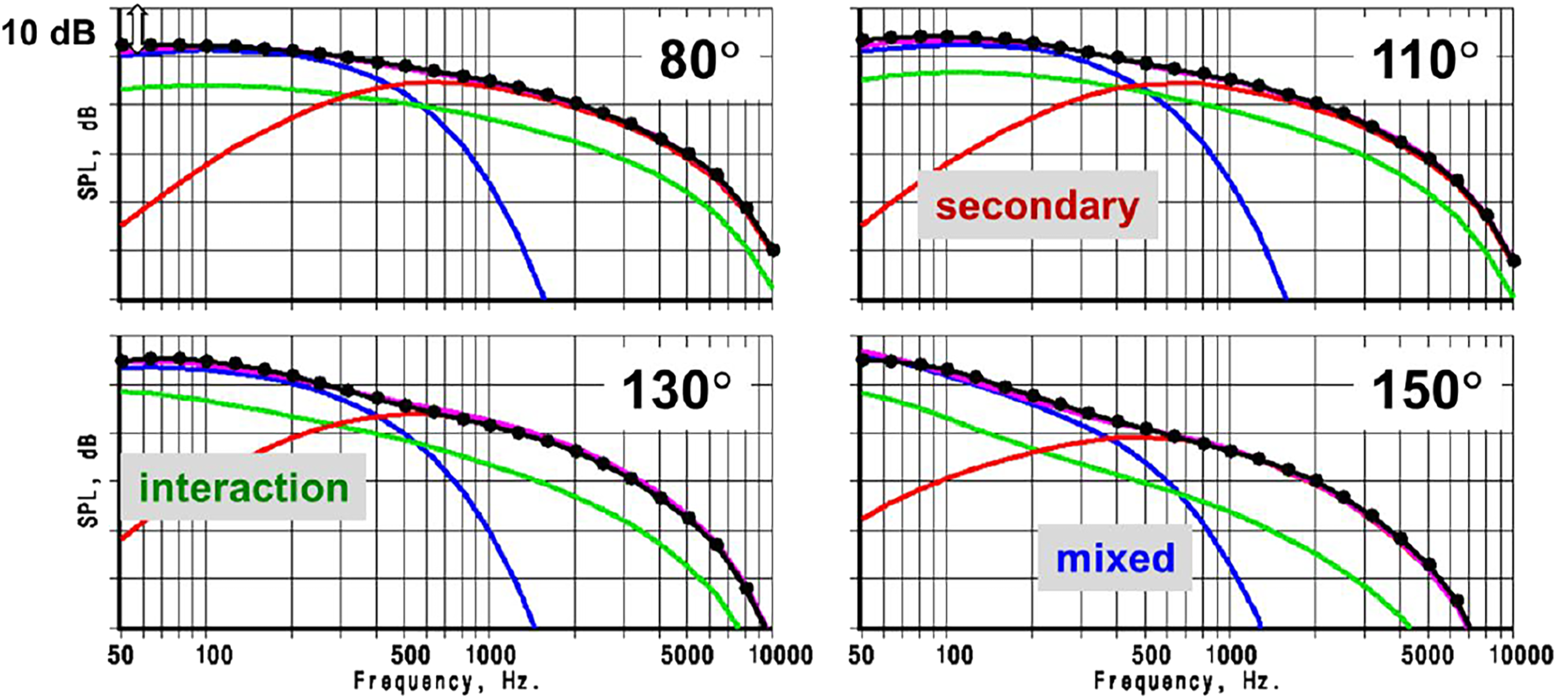

Next we consider the jet noise measured from a model scale dual-stream nozzle geometry and a turbofan engine, with the same nozzle configuration. As before for the turbojet engine (Figure 64), the model spectra are extrapolated to engine size. Figure 66 shows spectral comparisons at two power settings, low and high, and at two angles. Predicted spectra with the new method is also included (blue lines). Black lines and closed symbols represent engine data; the magenta line and open circles denote model scale data. There is good agreement between the predictions and model data, similar to the trends seen in Figure 65. There is good agreement at the lower frequencies for the two sets of data (denoted by red ovals), indicating the frequency ranges for which jet noise is dominant. It is evident now that the prediction method is applicable to turbofan engines as well.

Figure 66.

Comparison of static model scale and engine spectra for turbofan engine. Left: low power; right: high power. Black: engine data; magenta: model data; blue: prediction.

Figure 67 shows comparisons of predicted jet spectra with measured total noise from a static engine test at four different angles. The symbols denote data and the black lines are predicted jet spectra. There is good spectral agreement at the lower frequencies at all angles, where jet noise is dominant. The contributions from the non-jet sources are also highlighted; the magnitude and dominance of the non-jet component is clearly a function of angle, engine cycle conditions, engine size, design features, etc. The good agreement also enables the identification and quantification of the turbomachinery noise, which can be extracted through the subtraction of jet noise from the measured data.

Figure 67.

Comparison of spectral prediction with static engine data. Symbols: measured total spectra; lines: prediction. Red: secondary; blue: mixed; green: interaction; black: predicted total. High takeoff power.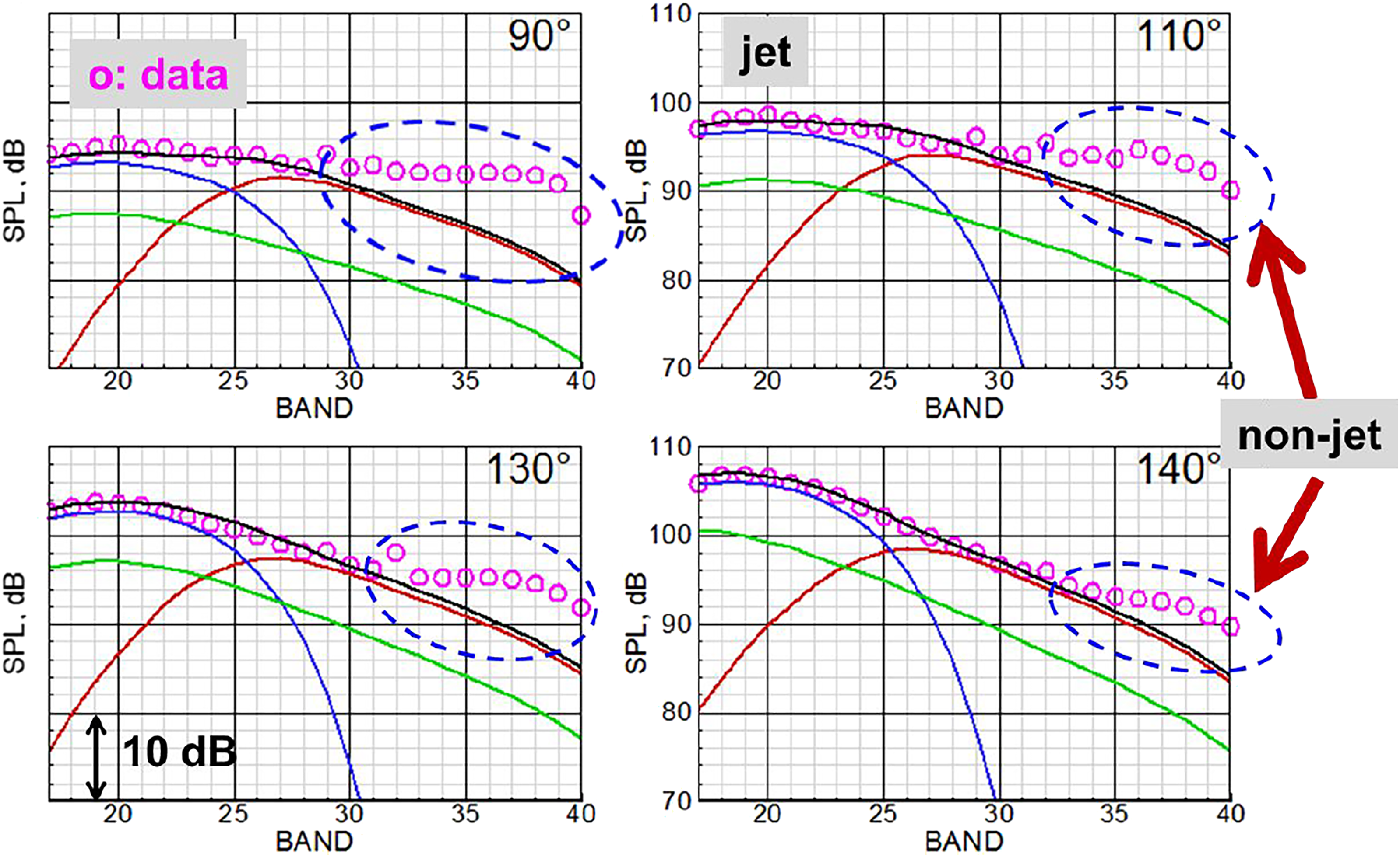

Finally, aircraft flyover cases are considered. Spectral predictions at the overhead microphone location, obtained with flush-mounted microphones, are presented. In an aircraft flyover test, additional sources associated with the airframe (landing gear, flap side edges, wing tip and trailing edge, etc.), jet flap interaction, and installation of the engine on an aircraft are also present. The airframe noise is measured at various airplane velocities and configurations, and scaling laws are established. Direct predictions of jet noise are made for the given cycle conditions and for the given airplane flight velocity. The extracted non-jet noise from static engine data is projected to the flyover geometry with appropriate corrections for sound propagation distance, for atmospheric attenuation, for propagation through the shear layer, etc. The logarithmic summation of these engine components together with the scaled airframe noise yields the predicted total airplane noise, which is compared with measurements. Figure 68 shows a typical example at maximum takeoff power by a modern high BPR engine. The landing gears are stowed and the flap extension is small. Consequently, the level of airframe noise is reduced. Spectral comparisons at six angles from 90° to 150° are displayed. The symbols denote measurements; red lines represent airframe noise; blue lines denote jet noise, and green lines denote non-jet noise. The black lines represent the predicted total airplane noise, which should be compared with the symbols. First of all, there is good spectral agreement at all angles. The level of the airframe noise is much lower than the measurements and is not important during takeoff. Jet noise is dominant up to ∼1500 Hz (band number = 32), as it matches the data well; the non-jet component becomes important at the higher frequencies. Similarly good agreement is demonstrated for other airplane/engine combinations from approach to takeoff power.

Figure 68.

Prediction of airplane flyover noise at takeoff power. Symbols: measured total spectra. Blue lines: predicted jet noise; red lines: measured airframe noise; green: projected non-jet noise; black lines: predicted total. High takeoff power.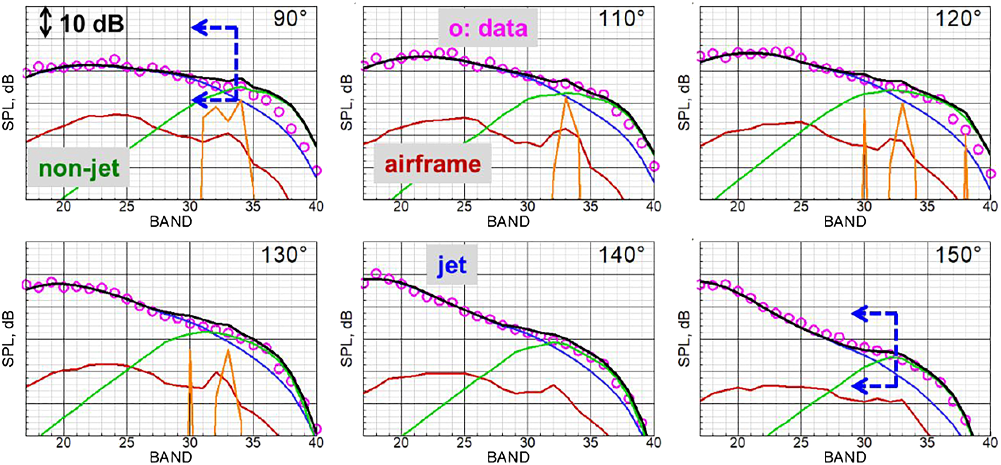

As stated in Viswanathan,¹⁶⁵ the practical benefits of the accurate prediction of jet noise are multifold: (1) it enables the identification and extraction of the individual noise components and helps establish their dominance as functions of frequency, angle and flight/engine conditions; (2) it allows the quantification of the sensitivities of the different components at various flight conditions; (3) it facilitates the deployment of resources to understand and reduce the dominant component at each certification location; and (4) finally, the new methodology is ideal for airplane-level design and trade studies, because of the minimal computer requirements and rapid turnaround time. Thus, the new prediction method is a powerful and improved tool that provides insights to the better understanding of the noise components and helps efforts directed at the reduction of aircraft noise.

Shock-associated noise from dual-stream jets

For typical dual-stream separate flow nozzles, the secondary pressure ratio (NPR_s) is always higher than the primary pressure ratio (NPR_p). At cruise altitude, both nozzles could be operated at super-critical pressure ratios because of the lower ambient pressure; this is especially true for the lower BPR engines developed in the 1970s and 1980s. As already stated, the fan pressure ratio and consequently the nozzle pressure ratios have decreased with increasing BPR. Still, the (NPR_s) becomes super-critical, though not as severe as in the older engines. The shock-associated noise impinges on the aircraft fuselage and is transmitted into the cabin. As one moves from the front of the airplane to the aft, cabin noise levels increase progressively. For wing-mounted engines, the most common configuration, there are three sources of cabin noise: the turbulent boundary layer over the fuselage, the turbulent mixing noise and shock-associated noise. Several flight tests have been conducted to quantify the contributions from these three sources; needless to say, the relative importance depends on the airplane, engine location and especially engine operating conditions. Shock-associated noise has been suspected to be a problem for certain aircraft, especially in the aft cabin. The reason for this was never fully understood.

One of the very few test programs that addressed the problem of shock-associated noise from dual-stream jets is that due to Tanna, Tam and Brown.¹⁶⁶ In two companion papers, Tam and Tanna^167,168 provided a theoretical explanation of the observed characteristics from the test program and developed a shock-cell model for the peak frequency and the intensity of the shock-associated noise. Even though the model of Tam¹⁵² has been very successful in describing the mechanism of noise generation from single-stream jets, the role of the inner shear layer in a dual-stream jet is not well understood. Furthermore, many of the studies performed in the 1970s and 1980s concentrated on jets with inverted velocity profiles (IVP, secondary stream faster than the primary stream), as the noise reduction potential of these jets was recognized for supersonic aircraft. However, the complexities and weight penalties associated with ducting the higher velocity stream to the secondary side have proven to be prohibitive and hence the IVP concept has not found application in jet engines. Therefore, a systematic study, with an emphasis on normal velocity profile (NVP) jets, is described here that sheds light on the mechanisms of generation of noise from dual-stream nozzles.

The cycle conditions in the database described in Viswanathan¹⁶¹ were carefully chosen, such that both streams were subsonic, both were supersonic, and either the primary or the secondary was subsonic and the other one was supersonic. A systematic variation of the primary and secondary NPR (or Mach number) ensured that key aspects of the effect of varying a particular parameter could be quantified; see Figure 2 in Viswanathan¹⁶¹ for the test matrix. The primary temperature ratios at different NPR_p correspond to an actual engine cycle. The area ratio is A_s/A_p = 3.0, which is representative of the engines with stronger shocks at cruise. The effects of different operating conditions in the two streams on both the turbulent mixing noise and shock-associated noise are evaluated under static condition as well as in the presence of an external co-flowing stream. A few salient findings are summarized below; see Viswanathan¹⁶¹ for more details.

The results indicate that the secondary-to-primary jet velocity ratio is an important parameter for mixing noise while its effect is negligible on shock-associated noise. The shock-associated noise, not surprisingly, is dependent on the geometric details of the nozzle. There are tremendous differences in the radiated noise depending upon the establishment of shocks in the primary, or secondary or both streams. When the primary stream is supersonic, with the secondary stream at subsonic or low supersonic Mach number, the shock-associated noise from the primary jet controls the radiated noise to low angles, with a substantial increase in the levels of the mixing noise at aft angles commensurate with the higher mixed velocity. The characteristics of the shock-associated noise are similar to those from a single jet (Figure 62) and the importance of the secondary shear layer is presumably diminished greatly. Dramatic differences occur when the secondary stream is supersonic and the primary stream is either subsonic or at a low supersonic Mach number. The emergence of shock-associated noise from the secondary stream becomes apparent in the forward angles. However, of greater significance is the radiation of shock-associated noise to aft angles, which becomes more pronounced with increasing Mach number in the secondary stream. This trend of two different shock components has not been reported in the past. This aft radiation is troublesome because this component is transmitted into the aft cabin of certain aircraft with engines mounted close to the fuselage. Conclusive evidence was presented that indicates that strong radiation to aft angles happens only when the secondary stream is supersonic, regardless of the Mach number of the primary stream. In this regard, the characteristics of the shock-associated noise from the secondary stream are very different from those of a single jet or a dual-stream jet with the shocks in the primary jet. Just as for a single jet, the effect of forward flight on mixing noise and shock-associated noise is very different. While there is a progressive reduction in levels of mixing noise with increasing free-stream velocity, there is amplification of the shock-associated noise. This is particularly so for the aft-radiated component of shock noise from the secondary stream. This effect could further exacerbate the interior noise in the aft cabin.

A collaborative effort with Professor Tam was undertaken to gain physical insights into this problem. Tam, Pastouchenko and Viswanathan¹⁶⁹ describe the computation of the shock-cell structure for the same geometry as in the tests. Tam, Pastouchenko and Viswanathan¹⁷⁰ used these computations for deducing the physics of noise generation and prediction. Tam, Pastouchenko and Viswanathan¹⁶⁹ noted that the shock cells in the supersonic secondary jet are generated primarily by the pressure mismatch at the nozzle exit. The methodology is to compute first the pressure mismatch at the nozzle exit. The shock cell structure is then determined computationally by solving the linearized RANS equations, satisfying the pressure mismatch condition at the nozzle exit of the secondary jet. Broadband shock cell noise may be regarded as the result of coherent scattering of the large turbulence structures by the shock cells as the former propagate downstream through the latter. Coherent scattering leads to strong directional radiation. For this reason, it is the spatially periodic components of the shock cell structure that are most relevant to shock cell noise prediction. Here, because of the complexity of the shock cell structure, the periodic components are found by computing the Fourier modes of the shock cell structure. The wave number spectrum of each Fourier mode in the shock cell noise producing region of the jet is then computed to identify the dominant spatially periodic components. The applicability of this approach is validated by using the dominant wave number found to calculate the frequencies at the peaks of the experimentally measured broadband shock cell noise spectra. Good agreements are found over a range of primary and secondary jet Mach numbers.

Tam, Pastouchenko and Viswanathan¹⁷⁰ sought to uncover the underlying physical mechanism for the two shock components, by considering a supersonic secondary stream and high subsonic primary stream. Figure 69 shows typical noise spectra from 50° to 130° in 10 degree increment, with the following jet conditions: M_p = 0.85, T_p/T_a = 2.26; M_s = 1.36, T_s/T_a = 1.0. The spectra from 50° to 80° contain a prominent peak, which is the principal and first broadband shock-cell peak and analogous to those of single-stream jets. The frequency of the spectral peak denoted by a small black arrow increases with inlet angle. The spectrum at 90° has two principal peaks; the second one is identified by an open arrow. The existence of two peaks can be seen at 100°. At angles larger than 100°, the maximum level of the of the first peak decreases rapidly. In contrast, the level of the second peak increases and peaks at 110°; beyond this angle, this peak level also starts to decrease, though it is still observable at 130°. An examination of the directivity of the maximum levels for the two components provides a clearer picture in Figure 70. The maximum levels of the first two peaks of the first broadband shock-cell component from 50° to 100° are plotted. The levels decrease with increasing angle, similar to the trends seen for single jets. Starting from 90°, the directivity of the second component is also plotted in Figure 70. The peak level increases, attains a maximum value between 110° and 120°, and then starts to decrease rapidly. This behavior is very different from what is observed for the first component and in single-stream jets.

Figure 69.

Noise spectra of dual-stream jet. M_p = 0.85, T_p/T_a = 2.26; M_s = 1.36, T_s/T_a = 1.0.

Figure 70.

Directivity of maximum sound pressure level of broadband shock-associated noise. M_p = 0.85, T_p/T_a = 2.26; M_s = 1.36, T_s/T_a = 1.0.

Tam, Pastouchenko and Viswanathan¹⁷⁰ proposed that both noise components are generated by the interaction of large turbulence structures in the inner and outer shear layers and the shock-cell structure in the secondary stream. The first component is generated in the outer mixing layer and the noise is radiated primarily to upstream angles, with the levels decreasing with increasing inlet angle. The second component is generated in the inner mixing layer and radiates mainly in the downstream direction. The noise intensity is low at 90°, increases with angle and exhibits a rapid roll-off at larger aft angles. A vortex sheet dual-stream model is developed to elucidate the noise generation, transmission and radiation processes. This model provides formulae for the peak frequencies and radiation for both components. Good agreements with measured data are obtained for different jet conditions. This model also indicates the existence of a roll-off of the noise generated in the inner shear layer: the source responsible for sound radiation to large inlet angles is moving at a subsonic speed relative to the supersonic secondary jet. This slower speed causes the disturbances to decay exponentially through the secondary jet, resulting in a reduction in radiated noise. Thus, this model provides an explanation for the experimentally observed characteristics. See this reference for complete details.

Summary

Research has been carried out over 70 years to understand the physical processes that lead to the generation and radiation of jet noise. There is no complete theory to date, attesting to the complicated nature of this problem in fluid dynamics. This fascinating challenge has drawn the attention of numerous theoreticians and experimentalists. Beginning in the 1950s, the acoustic analogy (with several variants) served as the dominant theory for over 50 years. However, by the mid-1970s, many researchers noted significant discrepancies between the classical theories and experimental data. The discovery of large-scale coherent structures, which were viewed as wave-packets, in turbulent jets gave rise to a new perspective. Tam¹⁷ was the first to clearly demonstrate that these structures are efficient generators of noise and constitute the dominant noise sources, especially in the downstream direction. There have been several experimental and theoretical developments related to the measurement and modeling of the source mechanisms associated with the large-scale structures, since this pioneering work.

Experimental measurements have shown that the mean flow as well as the turbulence statistics exhibit a self-similarity in the mixing layer, and another similarity in the fully developed jet. Based on these observations, Tam and Chen³⁵ and Tam, Golebiowski and Seiner³⁶ proposed that since noise is generated by the turbulence of the jet, the noise spectra generated by fine-scale and large-scale turbulence should also exhibit self-similarity. By examining a large set of supersonic jet noise data acquired at NASA Langley, Tam offered evidence that the turbulent mixing noise of high-speed jets does consist of two independent self-similar components. These two original findings by Tam have dramatically altered our view of the source mechanisms responsible for the generation of noise. To wit, jet turbulence consisting of both random fine-scale and coherent large-scale structures constitutes the sources of jet noise. This is a radical departure from the classical theories of jet noise.

The objective here is to create a document that synthesizes the characteristics of jet noise. Experimental evidence is compiled and collated to clarify several issues that could impact the spectra. The fundamental characteristics, once determined, serve as the foundation for real-world applications. This endeavor is facilitated by an extensive database acquired and validated to be of high quality, through the use of scaling methodology (Figures 7 and 29). It is established at the outset that the turbulent mixing noise is the dominant component even for fighter aircraft powered by turbojet engines, operated at off-design supersonic conditions during takeoff. All commercial turbofan engines are operated at subsonic Mach numbers even at maximum takeoff power. Therefore, the focus here is on turbulent mixing noise. The main results are enumerated below:

1. The Reynolds number decreases when a jet is heated at a fixed Mach number. When the value of the Reynolds number dips below a threshold value, the spectra of heated jets at lower angles exhibit an extra hump near the peak and the peak frequency moves to a lower value. Past theories attributed these trends as due to the appearance of a dipole source. Spectra acquired with nozzles of increasing diameters indicate that this is an artifact of low Reynolds number and that this hump disappears when larger nozzles, with Reynolds number greater than ∼400,000, are used. Consequently, there is no validity to the idea of the emergence of dipoles for heated jets.

2. The state of the boundary layer in model tests, either laminar or turbulent, has a negligible effect on the radiated spectra. Jets with thin laminar boundary layers do not generate elevated levels at higher frequencies. The nozzles of all engines are conical and have turbulent boundary layers. The state of the boundary layer has no relevance or impact for real engines.

3. The overall sound power (OAPWL) does not follow an exact eighth power law but exhibits a weak dependence on jet temperature ratio, with the value of the exponent decreasing slightly with jet temperature. The OASPL has a much stronger dependence, especially at the lower angles, with the velocity exponent decreasing from ∼8 for unheated jets to ∼5.5 at a stagnation temperature ratio of 3.2. The velocity exponent has a strong dependence on angle and temperature ratio. This temperature effect as an independent controlling parameter is a crucial new finding and was unrecognized for nearly 50 years since the formulation of the eighth power law.

4. Once the critical role of the temperature ratio on spectra is identified and isolated, it is straightforward to form new scaling laws that are valid for all angles with the current database. There are no multiplicative factors with adjustable constants for the spectrum functions; the spectrum function and the velocity exponent depend on the jet temperature ratio and the radiation angle. This relation represents the main difference between the current and the classical formulations. A single exponent collapses the entire spectrum from jets with different V_j/a, thereby obviating the need for disparate assumptions and tunable constants for different frequency regimes at any given angle. This practice, adopted in models based on classical theories, is perhaps the most unsatisfactory aspect as it destroys any semblance of a universal scaling law. The new scaling law has been derived from a comprehensive analysis of a large database. No claim is made as to any new breakthrough in the theoretical arena, as it is not based on any theoretical consideration.

5. The notion of moving sources immediately leads to a Doppler shift for frequency and a convective amplification factor for the noise radiated to the aft angles. With the aid of the current database, it is shown that the plain Strouhal number without any form of Doppler shift leads to excellent collapse of the spectra at all angles over the entire Strouhal number (raw frequencies from 200 Hz to 80 kHz) range. It is unambiguously demonstrated that the jet temperature, rather than the jet velocity, controls the spectral shape in the aft angles (Figures 26–28). There is no experimental evidence for the classical ideas of source convection together with flow/acoustic interaction and refraction as being responsible for the change in spectral shape from a broad spectrum at 90° (FSS) to the peaky shape (LSS) at large aft angles.

6. The spectral shape corresponds to that of the FSS spectrum at low angles at all jet conditions, for jets from single-stream, separate flow dual-stream, non-circular and confluent nozzle geometries. There is a family of peaky LSS shapes for single-stream jets, because of the effect of jet temperature: the spectral width at aft angles becomes narrower when the temperature is increased.

7. The scaling law also led to the discovery of the phenomenon of nonlinear propagation for heated subsonic jets (Figures 30–31). Nonlinear propagation is triggered for the turbulent mixing noise when the convective Mach number exceeds unity; this corresponds to a jet velocity of ∼1600 ft/sec. The precise condition that triggers nonlinear propagation for shock noise is not known.

8. The effects of forward flight have been quantified at several jet conditions and the flight velocity exponent has been calculated at all angles. As expected, the values of the exponents do not depend on jet conditions. Good spectral collapse at all frequencies, over the entire flight Mach number range of 0.0 – 0.32, is obtained with the plain Strouhal number, with (V_j) as the velocity scale. Use of the modified Strouhal number with (V_j – V_t) destroys the spectral collapse; therefore, the relative velocity is not the correct velocity scale.

9. A single equation describes the spectral characteristics at all angles, with and without forward flight. It is possible to make accurate absolute spectral predictions, as it involves only an inversion of the spectral scaling. The range of temperature ratios embedded in the method exceeds the operating conditions of all turbofan engines. A very advantageous feature is the following: it allows a clean prediction at low jet velocities for which accurate measurements would be impossible, especially with forward flight.

10. The idea of two distinct sources that are related to the fine-scale and large-scale turbulence of the jet plume has been investigated in great detail and reported in Tam et al.,^113,125,126 Viswanathan^92,93 and Viswanathan et al.¹¹². The convective Mach numbers covered a range of 0.28 – 1.69. Results from five different experimental techniques have been examined: (1) farfield spectral characteristics; (2) azimuthal and polar correlations in the farfield; (3) correlations of jet turbulence fluctuations and farfield sound; (4) measurement of source distributions with an elliptic mirror; and (5) space-time correlation measurements in the nearfield with a cage array, and nearfield-farfield correlations. Two distinctly different trends are observed in the angular ranges of 50° – ∼120° and ∼120° – 165° for all the parameters investigated with the above five approaches. The salient observations are mutually supporting, and the cumulative weight lends credence to the proposition that there are two distinct sources of turbulent mixing noise.

11. A large coherent region, with an axial extent from ∼13D to ∼31D, was discovered for all convective Mach numbers. A very high value of correlation/coherence (50%) prevails in a region with an axial extent of ∼15D for all jet velocities, for any single position at any axial location with (1) every other position in the nearfield, and (2) with farfield sound at aft angles ≥135° for unheated jets, and ≥120° for heated jets. This is a notable new finding and is quite remarkable. It is worth pointing out, that this large coherent source was completely missed in prior investigations with nearfield arrays because of the shorter axial extents of the arrays. It was also shown that large coherent structures could be responsible for noise radiated to angles close to the jet axis even at very low jet velocities. The farfield spectral shapes and correlations at these angles exhibit the same trends for convectively supersonic as well as very low velocity jets; this surprising finding suggests the primacy of the large scale structures in noise generation at all jet velocities. The modification of the noise characteristics by the beveled nozzle further reinforces this concept.

12. A model scale jet emits the same jet noise as a turbojet engine. The scaling law for single-stream jets has been extended to realistic dual-stream exhaust geometries of modern turbofan engines, and a new empirical prediction method has been developed. Good absolute spectral predictions have been demonstrated first at model scale for: (1) area ratio range of 2.6–8.0; (2) velocity ratio range of 0.6–1.1; (3) BPR range from 4.7 to 20.0; and (4) flight Mach number range of 0.0 – 0.32. See Viswanathan¹⁶⁵ for complete details. The same method is then applied to full-scale predictions, both from static engine tests and airplane flyover tests, with good spectral agreement.

13. Turbofan engines are invariably operated at supercritical pressure ratios during cruise, due to low ambient pressure at altitude. Shock-cells in the secondary stream generate two broadband shock-cell components, a new finding. The first component is generated in the outer mixing layer and the noise is radiated primarily to upstream angles, with the levels decreasing with increasing inlet angle. The second component is generated in the inner mixing layer and radiates mainly in the downstream direction. The noise intensity is low at 90°, increases with angle and exhibits a rapid roll-off at larger aft angles. The second component impinges on the aft fuselage and is transmitted into the aft cabin. The effect of forward flight amplifies this component, further exacerbating this problem for cabin noise.

The following thoughts on future research are offered in closing. The topic of Computational Aeroacoustics is not addressed here. High-fidelity numerical simulations with a fine grid could provide complete details of the flow field and the near field. Such simulations at high and low velocities could potentially shed light on the mechanisms and role of large-scale structures on noise generation and explain the experimental findings. Attempts at reduction of turbulent mixing noise at fixed bypass ratio have not been successful. Better insights to the flow features that could be modified in some fashion for noise reduction are essential.

Footnotes

Acknowledgments

It is a pleasure to acknowledge the outstanding support provided by the test crew at the Low Speed Aeroacoustic Facility of Boeing over several years. The author benefitted greatly from the numerous discussions with colleagues Don Boston and Jim Underbrink that resulted in improved and more capable measurement and data acquisition systems. The insights imparted by Dr. Philippe Spalart on boundary layer characteristics were invaluable. The long association from the mid-1980s with Professors Phil Morris and Dennis McLaughlin has been technically stimulating and fruitful. It has been a privilege and pleasure to collaborate with Professor Tam since the early 1990s; his drive and enthusiasm were infectious and inspirational. Thanks also to Dr. James Bridges and Dr. Nick Georgiadis of NASA Glenn for sharing the designs for the shock-free convergent-divergent nozzle contours. Technical interactions with numerous colleagues in industry, NASA and academia have been enriching. Finally, many thanks to the two Reviewers for their patience and perseverance in reading this long article and providing constructive suggestions.

Declaration of conflicting interests

The author(s) declared no potential conflicts of interest with respect to the research, authorship, and/or publication of this article.

Funding

The author(s) received no financial support for the research, authorship, and/or publication of this article.

ORCID iD

K Viswanathan

References

Lighthill

. On sound generated aerodynamically: I. general theory. Proc R Soc London A 1952; 211: 564–581.

Lighthill

. On sound generated aerodynamically: II. Turbulence as a source of sound. Proceedings of the Royal Society of London, Series A, Mathematical and Physical Sciences 1954; 222: 1–32.

Proudman

. The generation of noise by isotropic turbulence. Proceedings of the Royal Society of London, Series A 1952; A214: 119–132.

Philips

. On the generation of sound by supersonic turbulent shear layer. J Fluid Mech 1960; 9: 1–28.

Doak

. Acoustic radiation from a turbulent fluid containing foreign bodies. Proceedings of the Royal Society of London, Series A 1960; 254(1276): 129–145.

Ffowcs–Williams

. The noise from turbulence convected at high speed. Transaction of the Royal Society of London, Series A 1963; 255(1061): 469–503.

Ribner

. The generation of sound by turbulent jets. Advances in Applied Mechanics. New York: Academic Press, 1964, pp. 108–182

Lilley

. Aerodynamic noise. Noise mechanisms. London: AGARD-CP-131, 1974.

Lilley

. Jet noise classical theory and experiments, in aeroacoustics of flight vehicles: theory and practice. Noise sources. Washington, DC: NASA RP 1258, 1991

10.

Mollo-Christensen

. Jet noise and shear flow instability seen from an experimenter’s viewpoint. J Appl Mech 1967; 34: 1–7.

11.

Crow

Champagne

. Orderly structure in jet turbulence. J Fluid Mech 1971; 48: 547–591.

12.

Brown

Roshko

. On density effects and large structure in turbulent mixing layers. J Fluid Mech 1974; 64: 775–816.

13.

Mollo-Christensen

Narasimha

. Sound emission from jets at high subsonic velocities. J Fluid Mech 1960; 8(01): 49–60.

14.

Batchelor

Gill

. Analysis of the stability of axisymmetric jets. J Fluid Mech 1962; 14(04): 529–551.

15.

Michalke

. “A wave model for sound generation in circular jets,” Technical report, Deutsche Luft- und Raumfahrt. https://elib.dlr.de/63062/.

16.

Bishop

Williams

Smith

. On the noise sources of the unsuppressed high-speed jet. J Fluid Mech 1971; 50(01): 21–31.

17.

Tam

CKW

. Directional acoustic radiation from a supersonic jet generated by shear layer instability. J Fluid Mech 1971; 46(4): 757–768.

18.

Tam

CKW

. On the noise of a nearly ideally expanded supersonic jet. J Fluid Mech 1972; 51: 69–95.

19.

Chan

Westley

. Directional acoustic radiation generated by spatial jet instability. C.A.S.I. Transactions 1973; 6(1): 36–41.

20.

Morris

. A model for the structure of jet turbulence as a source of noise. Reston, SV: AIAA, 1974

21.

Morris

. Flow characteristics of the large-scale wave-like structure of a supersonic round jet. J Sound Vib 1977; 53: 223–244.

22.

Liu

JTC

. Developing large-scale wavelike eddies and the near jet noise field. J Fluid Mech 1974; 62: 437–464.

23.

Tam

CKW

. Supersonic jet noise generated by large scale disturbances. J Sound Vib 1975; 38(1): 51–79.

24.

McLaughlin

Morrison

Troutt

. Experiments on the instability waves in a supersonic jet and their acoustic radiation. J Fluid Mech 1975; 69(1): 73–95.

25.

Williams

JEF

Kempton

. The noise from the large-scale structure of a jet. J Fluid Mech 1978; 84(4): 673–694.

26.

Morris

Tam

CKW

. On the radiation of sound by the instability waves of a compressible axisymmetric jet. Mechanics of sound generation in flows. New York: Springer-Verlag, 1979.

27.

Tam

CKW

Morris

. The radiation of sound by the instability waves of a compressible plane turbulent shear layer. J Fluid Mech 1980; 98: 349–381.

28.

Seiner

McLaughlin

Liu

. Supersonic jet noise generated by large-scale instabilities. Washington, DC: NASA TP-2072, 1982.

29.

Tam

CKW

Burton

. Sound generated by instability waves of supersonic flows. Part 1: two dimensional mixing layers. Part 2: axisymmetric jets. J Fluid Mech 1984; 138: 249–295.

30.

Tam

CKW

Chen

Seiner

. Relationship between the instability waves and noise of high-speed jets. AIAA J 1992; 30(7): 1747–1752.

31.

Tam

CKW

. Jet noise generated by large-scale coherent motion. In: Hubbard

(ed). Aeroacoustics of flight vehicles: theory and practice, volume 1: noise sources. Washington, DC: NASA RP, 1991, pp. 311–390.

32.

Tam

CKW

. Supersonic jet noise. Annu Rev Fluid Mech 1995; 27: 17–43.

33.

Tam

CKW

. Jet noise: since 1952. Theor Comput Fluid Dynam 1998; 10: 393–405.

34.

Viswanathan

Czech

. Adaptation of the beveled nozzle for high-speed jet noise reduction. AIAA J 2011b; 49(5): 932–944.

35.

Tam

CKW

Chen

. Turbulent mixing noise from supersonic jets. AIAA J 1994; 32(9): 1774–1780

36.

Tam

CKW

Golebiowski

Seiner

. On the two components of turbulent mixing noise from supersonic jets. Reston, SV: AIAA Paper 96-1716, 1996.

37.

Viswanathan

. Analysis of the two similarity components of turbulent mixing noise. AIAA J 2002; 40(9): 1735–1744.

38.

Tam

CKW

Auriault

. Jet mixing noise from fine-scale turbulence. AIAA J 1999; 37(2): 145–153.

39.

Tam

CKW

Pastouchenko

Viswanathan

. Fine scale turbulence noise from hot jets. AIAA J 2005; 43(8): 1675–1683.

40.

Viswanathan

. Nozzle shaping for reduction of jet noise from single jets. AIAA J 2005; 43(5): 1008–1022.

41.

Tam

CKW

. A phenomenological approach to jet noise: the two-source model. Phil. Trans. R. Soc. A 2019; 377: 20190078.

42.

Viswanathan

. Mechanisms of jet noise generation: classical theories and recent developments. Int J Aeroacoustics 2009a; 8(4): 355–407.

43.

Morris

Viswanathan

. Jet noise. Noise sources in turbulent shear flows: fundamentals and applications, CISM courses and lectures. East Lansing, MI: Michigan State University, 2013, pp. 119–196.

44.

Shields

Bass

. Atmospheric absorption of high frequency noise and application to fractional-octave band. Washington, DC: NASA-CR 2760, 1977.

45.

Viswanathan

. Jet aeroacoustic testing: issues and implications. AIAA J 2003; 41(9): 1674–1689.

46.

Viswanathan

. Instrumentation considerations for accurate jet noise measurements. AIAA J 2006a; 44(6): 1137–1149.

47.

Viswanathan

. Best practices for accurate measurement of pure jet noise. Int J Aeroacoustics 2010a; 9(1): 145–206.

48.

Viswanathan

. Aeroacoustics of hot jets. J Fluid Mech 2004a; 516: 39–82.

49.

Fisher

Lush

Harper Bourne

. Jet noise. J Sound Vib 1973; 28(3): 563–585.

50.

Tanna

Dean

Fisher

. The influence of temperature on shock-free supersonic jet noise. J Sound Vib 1975; 39(4): 429–460.

51.

Tanna

. An experimental study of jet noise, Part I: turbulent mixing noise. J Sound Vib. 1977; 50(3): 405–428.

52.

Tester

Morfey

. Developments in jet noise modelling – theoretical predictions and comparisons with measured data. J Sound Vib 1976; 46(1): 79–103.

53.

Morfey

Szewczyk

Tester

. New scaling laws for hot and cold jet mixing noise based on a geometric acoustics model. J Sound Vib 1978; 61(2): 255–292.

54.

Goldstein

. An exact form of Lilley’s equation with a velocity quadrupole/temperature dipole source term. J Fluid Mech 2001; 443: 231–236.

55.

Bradshaw

. The effect of initial conditions on the development of a free shear layer. J Fluid Mech 1966; 26(2): 225–236

56.

Lau

. Effects of exit Mach number and temperature on mean-flow and turbulence characteristics in round jets. J Fluid Mech 1981; 105: 193–218.

57.

Lepicovsky

Ahuja

Brown

, et al. Acoustic control of free jet mixing. J Propul Power 1986; 2: 323–330.

58.

Lepicovsky

. Centerline Mach number characteristics of highly heated free jets. Reston, SV: AIAA-88-3612, 1988.

59.

Zaman

KBMQ

. Asymptotic spreading rate of initially compressible jets – experiment and analysis. Phys Fluid 1998; 10(10): 2652–2660.

60.

Moore

. The role of shear-layer instability waves in jet exhaust noise. J Fluid Mech 1977; 80(2): 321–367.

61.

Zaman

KBMQ

. Effect of initial condition on subsonic jet noise. AIAA J 1985; 23(9): 1370–1373.

62.

Zaman

KBMQ

. Flow field and near and far sound field of a subsonic jet. J Sound Vib 1986; 106(1): 1–16.

63.

Bridges

Hussain

AKMF

. Roles of initial condition and vortex pairing in jet noise. J Sound Vib 1987; 117(2): 289–311.

64.

Viswanathan

Clark

. Effect of nozzle internal contour on jet aeroacoustics. Int J Aeroacoustics 2004; 3(2): 103–135.

65.

Grosche

. Distribution of sound source intensities in subsonic and supersonic jets. AGARD Conference Proceedings 1973; 131.

66.

Jones

Launder

. Some properties of sink-flow turbulent boundary layers. J Fluid Mech 1972; 56: 337–351.

67.

Narasimha

Sreenivasan

. Relaminarization in highly accelerated turbulent boundary layers. J Fluid Mech 1973; 61: 417–447.

68.

Spalart

. Numerical study of sink-flow boundary layers. J Fluid Mech 1986; 172: 307–328.

69.

Brandt

. Relaminarized boundary layers subjected to adverse pressure gradients. PhD Thesis. Cambridge: University of Cambridge, 1993.

70.

Mukund

. Relaminarization in a short acceleration zone on a convex surface. PhD Thesis. India: Department of Aerospace Engineering, Indian Institute of Science, 2002.

71.

Zaman

KBMQ

. Initial boundary layer state of typical model-scale jet nozzles and its impact on noise. Int J Aeroacoustics 2023; 22(5-6): 500–529.

72.

Viswanathan

. Scaling laws and a method for identifying components of jet noise. AIAA J 2006b; 44(10): 2274–2285.

73.

Viswanathan

. Improved method for prediction of noise from single jets. AIAA J 2007a; 45(1): 151–161.

74.

Viswanathan

. The role of jet temperature ratio in correlating jet noise. AIAA J 2009b; 47(5): 1090–1106.

75.

Hoch

Duponchel

Cocking

, et al. Studies of the influence of density on jet noise. J Sound Vib 1973; 28(4): 649–668.

76.

Morfey

. Amplification of aerodynamic noise by convected flow inhomogeneities. J Sound Vib 1973; 31: 391–397.

77.

Goldstein

. A unified approach to some recent developments in jet noise theory. Int J Aeroacoustics 2002; 1: 1–16.

78.

Lush

. Measurements of subsonic jet noise and comparison with theory. J Fluid Mech 1971; 46(3): 477–500.

79.

Viswanathan

. Does a model scale nozzle emit the same jet noise as a jet engine? AIAA J 2008a; 46(2): 336–355.

80.

Viswanathan

Alkislar

Czech

. Characteristics of the shock noise component of jet noise. AIAA J 2010; 48(1): 25–46.

81.

Petitjean

Viswanathan

McLaughlin

. Acoustic pressure waveforms measured in high speed jet noise experiencing nonlinear propagation. Int J Aeroacoustics 2006; 5(2): 193–215.

82.

Saxena

Morris

Viswanathan

. Algorithm for the nonlinear propagation of broadband jet noise. AIAA J 2009; 47(1): 186–194.

83.

Morfey

Howell

. Nonlinear propagation of aircraft noise in the atmosphere. AIAA J 1981; 19: 986–992.

84.

Viswanathan

Czech

. Measurement and modeling of effect of forward flight on jet noise. AIAA J 2011a; 49(1): 216–234.

85.

Amiet

. Correction of open jet wind tunnel measurements for shear layer refraction. Reston, SV: AIAA paper 75-532, 1975.

86.

Amiet

. Refraction of sound by a shear layer. J Sound Vib 1978; 58(4): 467–482.

87.

Anon . Gas turbine exhaust noise prediction. Warrendale, Pennsylvania: SAE ARP876, 1994.

88.

Potter

. An investigation to locate the acoustic sources in high speed jet exhaust stream. El Segundo, CA: Wyle Laboratories Technical Report WR 68-4, 1968.

89.

MacGregor

Simcox

. The location of acoustic sources in jet flows by means of the “wall isolation” technique. Reston, SV: AIAA Paper 73-1041, 1973.

90.

Billingsley

Kinns

. The acoustic telescope. J Sound Vib 1976; 48: 485–510.

91.

Fisher

Harper-Bourne

Glegg

SAL

. Jet engine noise source location: the polar correlation technique. J Sound Vib 1977; 51(1): 23–54.

92.

Viswanathan

. Investigation of the sources of jet noise. Reston, SV: AIAA Paper 2007-3601, 2007b.

93.

Viswanathan

. Investigation of noise source mechanisms in subsonic jets. AIAA J 2008b; 46(8): 2020–2032.

94.

Siddon

. Noise source diagnostics using causality correlations. Dorchester, UK: AGARD CP 131, 1973.

95.

Seiner

Reethof

. On the distribution of source coherency in subsonic jets. Reston, SV: AIAA Paper 74-4, 1974.

96.

Maestrello

. Two-point correlations of sound pressure in the far field of a jet: experiment. Washington, DC: NASA TM 72835, 1976.

97.

Laufer

Schlinker

Kaplan

. Experiments on supersonic jet noise. AIAA J 1976; 14: 489–497.

98.

Armstrong

Michalke

Fuchs

. Coherent structures in jet turbulence and noise. AIAA Journal 1977; 15(7): 1011–1017.

99.

Fuchs

. On the application of acoustic “mirror”, “telescope” and “polar correlation” techniques to jet noise source location. “Telescope”, and “Polar Correlation” Techniques to Jet Noise Source Location,” J. Sound and Vibration 1978; 58(1): 117–126.

100.

Juve

Sunyach

Comte-Bellot

. Filtered azimuthal correlations in the acoustic farfield of a subsonic jet. AIAA J 1979; 17(1): 112–113.

101.

Bonnet

CMT

Fisher

. Correlation techniques and modal decomposition analysis for the detection of azimuthally coherent structures in jet flows. J Sound Vib 1979; 66: 545–555.

102.

Schaffar

. Direct measurements of the correlation between axial in-jet velocity fluctuations and far-field noise near the axis of a cold jet. J Sound Vib 1979; 64: 73–83.

103.

Ahuja

Lepicovsky

Tam

CKW

, et al. Tone-excited jets: theory and experiments. Washington, DC: NASA CR 3538, 1982.

104.

Panda

Seasholtz

. Experimental investigation of density fluctuations in high-speed jets and correlation with generated noise. J Fluid Mech 2002; 450: 97–130.

105.

Panda

Seasholtz

Elam

. Investigation of noise sources in high-speed jets via correlation measurements. J Fluid Mech 2005; 537: 349–385.

106.

Panda

. Experimental investigation of turbulent density fluctuations and noise generation from heated jets. J Fluid Mech 2007; 591: 73–96.

107.

Bridges

Wernet

. Measurements of the aeroacoustic sound source in hot jets. Reston, SV: AIAA Paper 2003-3130, 2003.

108.

Jordan

Tinney

Delville

, et al. Low dimensional signatures of the sound production mechanisms in subsonic jet: towards their identification and control. Reston, SV: AIAA Paper 2005-4647, 2005.

109.

Doty

McLaughlin

. Space-time correlation measurements of high-speed axisymmetric jets using optical deflectometry. Exp Fluid 2005; 38: 415–425.

110.

Bridges

. Effect of heat on space-time correlations in jets. Reston, SV: AIAA Paper 2006-2534, 2006.

111.

Jordan

. Analysis techniques for aeroacoustics: noise source identification. Noise sources in turbulent shear flows: fundamentals and applications, CISM courses and lectures. East Lansing, MI: Michigan State University, 2013, pp. 197–288.

112.

Viswanathan

Underbrink

Brusniak

. Space-time correlation measurements in near fields of jets. AIAA J 2011; 49(8): 1577–1599.

113.

Tam

CKW

Viswanathan

Ahuja

, et al. The sources of jet noise: experimental evidence. J Fluid Mech 2008b; 615: 253–292.

114.

Seiner

PontonJansen

MKBJ

Lagen

. The effects of temperature on supersonic jet noise emission. Reston, SV: AIAA Paper 92–2046, 1992.

115.

Norum

Brown

. Simulated high speed flight effects on supersonic jet noise. Reston, SV: AIAA Paper 93–4388, 1993.

116.

Morris

. A note on noise generation by large scale turbulent structures in subsonic and supersonic jets. Int J Aeroacoustics 2009; 8(4): 301–315.

117.

Ribner

. Two-point correlations of jet noise. J Sound Vib 1978; 56(1): 1–19.

118.

Michel

. Influence of source interference on the directivity of jet noise. Reston, SV: AIAA Paper 2007-3648, 2007.

119.

Seasholtz

Panda

Elam

. Rayleigh scattering diagnostics for dynamic measurement of velocity fluctuations in high speed jets. Reston, SV: AIAA Paper 2001–0847, 2001.

120.

Seasholtz

Panda

Elam

. Rayleigh scattering diagnostics for measurement of velocity and density fluctuation spectra. Reston, SV: AIAA Paper 2002–0827, 2002.

121.

Schlinker

Petersen

Kaplan

. Enhancement of directional microphone measurements. Reston, SV: AIAA Paper 73-1040, 1973.

122.

Chu

Laufer

Kao

. Noise source distribution in subsonic jets. Proceedings of the 1972 international conference on noise control engineering, Washington, DC, 4–6 October 1972.

123.

Viswanathan

. Distributions of noise sources in heated and cold jets: are they different? Int J Aeroacoustics 2010b; 9(5): 589–625.

124.

Witze

. Centerline velocity decay of compressible free jets. AIAA J 1974; 12(4): 417–418.

125.

Tam

CKW

Pastouchenko

Viswanathan

. Continuation of the near acoustic field of a jet to the far field. Part I: theory. Reston, SV: AIAA/CEAS Paper 2010-3728, 2010.

126.

Tam

CKW

Viswanathan

Pastouchenko

, et al. Continuation of the near acoustic field of a jet to the far field. Part II: experimental validation and noise source characteristics. Reston, SV: AIAA/CEAS Paper 2010-3729, 2010.

127.

. Investigation of the noise fields of supersonic axisymmetric jet flows. Ph. D. Thesis. Syracuse, NY: Syracuse University, 1971.

128.

Troutt

McLaughlin

. Experiments on the flow and acoustic properties of a moderate-Reynolds-number supersonic jet. J Fluid Mech 1982; 116: 123–156.

129.

Hileman

Thurow

Samimy

. Exploring noise sources using simultaneous acoustic measurements and real-time flow visualizations in jets. AIAA J 2002; 40(12): 2382–2392.

130.

Hileman

Thurow

Caraballo

, et al. Large-scale structure evolution and sound emission in high-speed jets: real-time visualization with simultaneous acoustic measurements. J Fluid Mech 2005; 544: 277–307.

131.

Suzuki

Colonius

. Instability waves in a subsonic round jet detected using a near-field phased microphone array. J Fluid Mech 2006; 565: 197–226.

132.

Reba

Narayanan

Colonius

, et al. Modeling jet noise from organized structures using near-field hydrodynamic pressure. Reston, SV: AIAA/CEAS Paper 2005-3093, 2005.

133.

Reba

Simonich

Schlinker

. Measurement of source wave-packets in high-speed jets and connection to far-field sound. Reston, SV: AIAA/CEAS Paper 2008-2891, 2008.

134.

Reba

Simonich

Schlinker

. Radiated by large-scale wave-packets in subsonic and supersonic jets. Reston, SV: AIAA/CEAS Paper 2009-3256, 2009.

135.

Tinney

Jordan

Delville

, et al. A time-resolved estimate of the turbulence and source mechanisms in a subsonic jet flow. Reston, SV: AIAA 2006-621, 2006.

136.

George

Wänström

Jordan

. Identifying aeroacoustic sources. Reston, SV: AIAA/CEAS Paper 2007-3603, 2007.

137.

Laurendeau

Jordan

Delville

, et al. Nearfield-farfield correlations in subsonic jets: what can they tell us? Reston, SV: AIAA/CEAS Paper 2007-3614, 2007.

138.

Guitton

Kerhervé

Jordan

, et al. The sound production mechanism associated with coherent structures in subsonic jets. Reston, SV: AIAA/CEAS Paper 2008-2892, 2008.

139.

Tam

CKW

. Mach wave radiation from high-speed jets. AIAA J 2009; 47(10): 2440–2448.

140.

Harper-Bourne

Fisher

. The noise from shock waves in supersonic jets. AGARD-CP 1973; 131: 1–13.

141.

Tanna

. An experimental study of jet noise. Part II: shock associated noise. J Sound Vib. 1977; 50(3): 429–444.

142.

Seiner

Norum

. Experiments on shock associated noise of supersonic jets. Reston, SV: AIAA paper 79-1526, 1979.

143.

Seiner

Norum

. Aerodynamic aspects of shock containing jet plumes. Reston, SV: AIAA paper 80-0965, 1980.

144.

Norum

Seiner

. Measurements of static pressure and far field acoustics of shock-containing supersonic jets. Washington, DC: NASA TM 84521, 1982a.

145.

Norum

Seiner

. Broadband shock noise from supersonic jets. AIAA J 1982b; 20: 68–73.

146.

Tam

CKW

Tanna HK . Shock associated noise of supersonic jets from convergent-divergent nozzles. J Sound and Vib. 1982; 81(3): 337–358.

147.

Seiner

. Advances in high speed jet aeroacoustics. Reston, SV: AIAA paper 84-2275, 1984.

148.

Seiner

. Acoustic near-field properties associated with broadband shock noise. AIAA J 1984; 22(9): 1207–1215.

149.

Norum

Shearin

. Effects of simulated forward flight on the structure and noise of an underexpanded jet. Washington, DC: NASA TP-2308, 1984.

150.

Yamamoto

Brausch

Janardan

, et al. Experimental investigation of shock-cell noise reduction for single-stream nozzles in simulated flight”, Test nozzles and acoustic data. In: Comprehensive data report. Washington, DC: NACA CR-168234, 1984.

151.

Tam

CKW

. The shock-cell structures and screech tone frequencies of rectangular and non-axisymmetric supersonic jets. J Sound Vib 1988; 121(1): 135–147.

152.

Tam

CKW

. Stochastic model theory of broadband shock associated noise from supersonic jets. J Sound Vib 1987; 116(2): 265–302.

153.

Tam

CKW

. Broadband shock-associated noise of moderately imperfectly expanded supersonic jets. J Sound Vib 1990; 140(1): 55–71.

154.

Tam

CKW

. Broadband shock associated noise from supersonic jets measured by a ground observer. AIAA J 1992; 30: 2395–2401.

155.

Tam

CKW

Jackson

Seiner

. A multiple-scales model of the shock-cell structure of imperfectly expanded supersonic jets. J Fluid Mech 1985; 153: 123–149.

156.

Tam

CKW

Seiner

. Proposed relationship between broadband shock associated noise and screech tones. J Sound Vib 1986; 110(2): 309–321.

157.

Tam

CKW

Ahuja

Jones

. Screech tones from free and ducted supersonic jets. AIAA J 1994; 32(5): 917–922.

158.

Raman

. Advances in understanding supersonic jet screech: review and perspective. Prog Aero Sci 1998; 34: 45–106.

159.

Raman

. Supersonic jet screech: half-century from Powell to the present. J Sound Vib 1999; 225(3): 543–571.

160.

. An empirical model for prediction of coaxial jet noise in ambient flow. Reston, SV: AIAA Paper 1986–1912, 1986.

161.

Viswanathan

. Parametric study of noise from dual-stream nozzles. J Fluid Mech 2004b; 521: 35–36.

162.

Viswanathan

Czech

Lee

. Toward prediction of dual-stream jet noise: database generation. AIAA J 2011; 49(12): 2695–2712.

163.

Fisher

Preston

Bryce

. A modelling of the noise from simple coaxial jets, Part I: with unheated primary flow. J Sound Vib 1998a; 209: 385–403.

164.

Fisher

Preston

Mead

. A modelling of the noise from simple coaxial jets, Part II: with heated primary flow. J Sound Vib 1998b; 209: 405–417.

165.

Viswanathan

. Progress in prediction of jet noise and quantification of aircraft/engine noise components. Int J Aeroacoustics 2018; 17(4-5): 339–379.

166.

Tanna

Brown

Tam

CKW

. Shock associated noise of inverted profile coannular jets, Part I: experiments. J Sound Vib 1985; 98(1): 95–113.

167.

Tam

CKW

Tanna

. Shock associated noise of inverted profile coannular jets, Part II: condition for minimum noise. J Sound Vib 1985a; 98(1): 115–125.

168.

Tam

CKW

Tanna

. Shock associated noise of inverted-profile coannular jets, part III: shock structure and noise characteristics. J Sound Vib 1985b; 98(1): 127–145.

169.

Tam

CKW

Pastouchenko

Viswanathan

. “Computation of shock-cell structure of dual-stream jets for noise prediction,”. AIAA J 2008a; 46(11): 2857–2867.

170.

Tam

CKW

Pastouchenko

Viswanathan

. Broadband shock-cell noise from dual stream jets. J Sound Vib 2009; 324: 861–891.