The role of embedded swirl in shear layer on turbulent jet mixing and noise

Abstract

The concept of thin-layer swirl as a means of turbulent jet mixing and noise control is investigated. Swirl is introduced at the exit of a conical nozzle through 12 short vanes which impart angular momentum primarily to the outer shear layer. In addition to the uniform swirl (case m = 0) design, three azimuthally modulated swirl configurations are created by varying the exit vane angle. To investigate the development of the small disturbances, the spatial linear instability analysis is performed on an inviscid parallel jet with thin-layer swirl to identify the unstable modes and estimate their spatial growth rates. The azimuthal modes, m = $= \pm 1, \pm 2, a n d \pm 3$ over a range of swirl number S are investigated. For low–moderate swirl, the negative helical modes (m < 0) are more spatially unstable than their positive counterparts; as swirl increases, the modal ordering reverses, with positive modes (m > 0) becoming dominant. High-order LES is used to assess how thin-layer swirl influences jet mixing and noise. Entrainment is quantified using the radial-velocity method and thin-layer swirl cases show a modest enhancement over a plain jet. The simulations show that the uniform swirl case (m = 0) achieves stronger mixing than the modulated designs (m = 1,2,3). Far-field acoustics is estimated by Ffowcs Williams-Hawkings (FWH) method and it shows a net OASPL reduction of 2–4 dB at $θ = 60 °$ and $90 °$ . The gross thrust penalty for introducing low-aspect ratio swirl vanes at the nozzle exit is about 7-11%. Future work targets the optimization of vane geometry and swirl strength to retain acoustic benefits while reducing thrust loss.

Keywords

jet instability mixing enhancement incompressible round jet swirling shear layer noise reduction entrainment thrust penalty

Introduction

Jet noise remains a primary concern in sustainable aviation and the aeroacoustics community. Active and passive flow control methods such as chevrons and tabs can broaden the shear layer and promote mixing to reduce certain noise components.^1–4 They often incur penalties in thrust and cruise efficiency, and their broadband impact is mixed across operating conditions. Application of chevrons to supersonic jets has limited effect on noise reduction and screech frequency. An alternative approach is to manipulate the shear layer directly by introducing swirl, which can enhance entrainment and alter noise generation mechanisms. Conventional “bulk” swirl rotates the entire core and tends to produce significant thrust loss and low-frequency amplification which is undesirable for practical systems. Co-axial swirl jets with installed swirl vanes have been studied by Schwartz,⁵ Lu et al.,⁶ Papamoschou,⁷ Balakrishnan & Srinivasan.⁸ The current study examines a thin-layer swirl concept in which swirl is introduced only in a narrow annulus near the nozzle lip, leaving the core nearly rotation-free. The idea is to trigger centrifugal instability waves in the outer shear layer where mixing noise is generated, while minimizing axial-to-azimuthal momentum redirection in the core. We consider both a uniform thin-layer swirl and azimuthally modulated variants (of low-order: with m = 1,2,3).

It is broadly agreed that turbulent mixing is the dominant source of the jet noise. which is governed primarily by the jet parameters such as jet velocity, temperature, and nozzle pressure ratio.^9–11 In Lighthill’s acoustic analogy,^12,13 the classic eighth-power scaling law implies that the acoustic power of a turbulent jet varies as $M_{j}^{8}$ . Therefore, lowering the effective jet Mach number by enhancing jet entrainment and mixing is the promising tool to reduce jet noise.

Acoustic radiation from jets is tightly linked to the hydrodynamic instabilities. Beginning with Rayleigh¹⁴ who derived the inviscid stability criterion for axisymmetric disturbances of non-swirling jets, research have been extended to the analysis of swirling jets which shows the coupling effect of centrifugal and Kelvin-Helmholtz instabilities. With the identification of large-scale coherent structures in shear layers and advances in precision acoustics and computation, attention has focused on the sources of turbulent mixing noise.^15,16 Swirl is a source that tends to weaken the large-scale structures in the shear layer depending on the swirl strength and triggers centrifugal instability waves. It creates the vortex breakdown in high-intensity swirling jets and suppresses vortex pairing. These changes are accompanied by mixing enhancement and greater momentum thickness compared to the non-swirling jets. It is commonly agreed that the primary sources of turbulent mixing noise generation are large- and fine-scale dynamics in the shear layer. understanding their stability characteristics is therefore essential for both swirling and non-swirling jets. Linear stability analysis is used as a simple but robust method to achieve this goal.^17–19

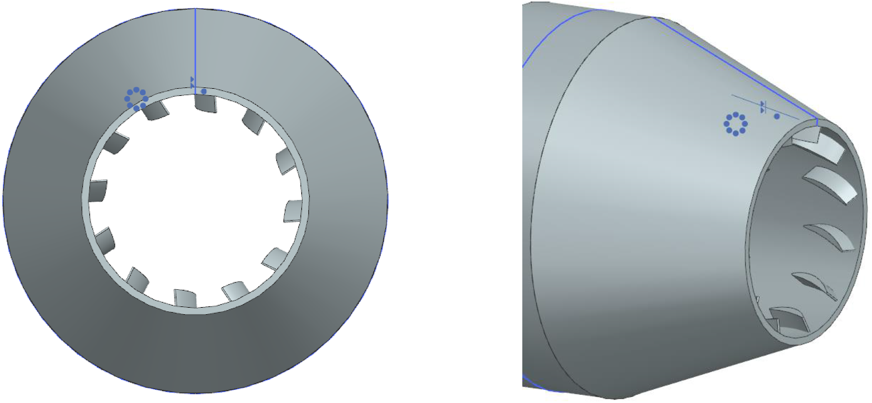
The concept of boundary-layer (thin-layer) swirl inside a supersonic nozzle was first applied to under-expanded supersonic rectangular nozzles by Han et al.,²⁰ who showed that exit-plane swirl excites centrifugal instability in the shear layer, enhances mixing, and incurs a gross thrust penalty of about 5.1% for a plain rectangular nozzle and 4.9% for a notched rectangular nozzle. Rahmani et al.²¹ extended the concept to an axisymmetric CD nozzle in supersonic flow using combined simulations and experiments, reporting up to 3 dB SPL reduction in the farfield across a broad Strouhal number range with <5% gross thrust loss. We investigate an embedded thin-layer swirl concept in low-subsonic jets (M <0.3) using linear spatial stability analysis and high-order LES on a simplified geometry. Low-profile, swirl-generating vanes are placed at the nozzle exit (as shown in Figure 1) to impart angular momentum primarily to the boundary layer. The intended mechanism is to trigger centrifugal instability and establish a radial pressure gradient across the shear layer that promotes entrainment and mixing while minimizing impact on the jet core. The results highlight the potential of thin-layer swirl for mixing and noise control.

Figure 1.

The CAD model of embedded low-profile swirl-generating vanes at nozzle exit.

The motivation of the current work is twofold: (i) Assess whether thin-layer swirl can increase entrainment and reduce farfield noise while producing a modest thrust loss penalty. (ii) Quantify how swirl strength and azimuthal modulation influence near-field instability, downstream evolution, and radiated noise. To address these, we combine high-order large-eddy simulation (LES) with linear spatial stability analysis to analyze the entrainment, acoustics, and thrust loss.

In this paper, we establish the exit-plane structure of the tangential flowfield for a uniform swirl and low-order azimuthal modulations (m = 1,2,3), and we quantify the time-averaged flowfield for a low-speed subsonic jet. A linear spatial stability study of inviscid swirling jets was conducted and the spatial amplification rate are presented at different swirl strength. The growth of normalized mass flow rate along the jet axis is presented by using the radial-velocity method. Farfield noise spectra reveal a net OASPL reduction driven by low–mid-frequency decreases with a modest high-frequency rise.

Spatial stability analysis

The linear spatial stability analysis is used to identify the unstable modes and their spatial growth characteristics. The analysis is performed on a top-hat parallel axial flow with a Rankine vortex swirl profile. The embedded swirl layer starts at radius R₀ and stretches to the nozzle lip at R. Hence, $R - R_{0}$ denotes the radial extent of the embedded swirling shear layer. The flow outside the nozzle is assumed to be irrotational and a potential vortex swirl distribution was used. The fluid is assumed to be inviscid and incompressible, since the swirling jet (or wake) spread mechanism is mainly pressure-driven in the nearfield, and the dynamics of the small disturbances are not dominated by fluid viscosity (Figure 2).

Figure 2.

The base-flow model of a thin-layer embedded swirl in a round jet with co-flowing external stream²⁷.

Therefore, the unperturbed velocity profile of the base flow, $\vec{\bar{V}} = (U, V, W)$ , in the three regions are written as:

U = U_{j 0}, V = 0, W = 0 (0 \leq r \leq R_{0})

(1a)

U = U_{j 0}, V = 0, W = Ω (r - R_{0}) (R_{0} \leq r \leq R)

(1b)

U = U_{\infty}, V = 0, W = (\frac{R}{r}) Ω (R - R_{0}) (r \geq R)

(1c)

where

U

V

and

W

denote the axial, radial and azimuthal velocity components, respectively.

U_{\infty}

is the freestream axial velocity,

U_{j 0}

is the axial velocity at the nozzle exit, and

Ω

is the angular velocity of the solid-body rotation in the thin shear layer. The small perturbations are present as normal modes:

{\hat{u}, i \hat{v}, \hat{w}, p^{'}} \exp [i (α x + m θ - ω t)] = {\hat{u}, i \hat{v}, \hat{w}, p^{'}} \exp {i [α (x - c t) + m θ]}

(2)

Where

\hat{u}, \hat{v}, \hat{w}, \hat{p}

are the amplitudes of the three fluctuating components of velocity and pressure. Axial wave number

α

is defined as

\frac{2 π}{λ}

, where

λ

is the disturbance axial wavelength,

m

is the azimuthal wave number (m = 0: axisymmetric; m = ±1: helical modes), and

ω

is the disturbance angular frequency. The phase speed c is the ratio of

ω / α

. In the spatial instability analysis,

ω

is assumed to be real and

α

is assumed to be complex, i.e.,

α = α_{r} + i α_{i}

, where

α_{r}

is the real axial wave number and

α_{i}

is the spatial amplification rate.

The fluid is assumed to be inviscid and incompressible, and the governing equations are Euler momentum equation and continuity equation in cylindrical coordinates.

\frac{\partial V}{\partial t} + (V \cdot \nabla) V = - \frac{1}{ρ} \nabla P

(3)

\nabla . V = 0

(4)

Where

V

is the velocity vector,

ρ

is the fluid density, and

P

is the fluid static pressure. The instantaneous flowfield is assumed to be the sum of the time-averaged (or the mean) flowfield and the contribution from the flow fluctuations, described by:

V = \bar{V} + V^{'}

(5)

P = \bar{P} + p^{'}

(6)

where

\bar{V}

denotes the time-averaged velocity vector, and

\bar{P}

is the local time-averaged static pressure field.

V^{'}

and

p^{'}

denote the fluctuations in velocity and pressure field, respectively.

The linearized perturbation equations of the momentum and continuity equations for incompressible inviscid fluids in cylindrical coordinates are:

A \hat{u} + \frac{\partial U}{\partial r} \hat{v} + α \hat{p} = 0

(7a)

- A \hat{v} - \frac{2 W}{r} \hat{w} + \frac{d \hat{p}}{d r} = 0

(7b)

(\frac{\partial W}{\partial r} + \frac{W}{r}) \hat{v} + A \hat{w} + \frac{m}{r} \hat{p} = 0

(7c)

α \hat{u} + \frac{\hat{v}}{r} + \frac{d \hat{v}}{d r} + \frac{m}{r} \hat{w} = 0

(7d)

Where

A = α U - ω + m W / r

. The perturbation equations can be reduced to a single linear second-order ordinary differential equation in terms of

\hat{u}

α^{2} [A^{2} - \frac{2 W}{r} (\frac{\partial W}{\partial r} + \frac{W}{r})] \frac{d}{d r} {\frac{A \frac{d (A \hat{u})}{d r} + \frac{2 m A W}{r^{2}} \hat{u}}{α^{2} [A^{2} - \frac{2 W}{r} (\frac{\partial W}{\partial r} + \frac{W}{r})]}} + \frac{A}{r} \frac{d (A \hat{u})}{d r} - \frac{m}{r} (\frac{\partial W}{\partial r} + \frac{W}{r}) \frac{d (A \hat{u})}{d r} + \frac{2 m A W}{r^{3}} \hat{u} - \frac{m^{2} A^{2}}{r^{2}} \hat{u} - α^{2} [A^{2} - \frac{2 W}{r} (\frac{\partial W}{\partial r} + \frac{W}{r})] \hat{u} = 0

(8)

To derive a uniformly consistent solution throughout the three regions, the solutions need to be matched at the two boundaries by imposing dynamic and kinematic boundary condition. By applying the dynamic boundary condition at the matching radius, i.e., $r = R_{0}$ and $r = R$ , we obtain:

{\bar{P}}_{+} (r + δ) + {p_{+}}^{'} (r + δ) = {\bar{P}}_{-} (r + δ) + {p_{-}}^{'} (r + δ)

(9)

Where the subscripts

+

and

-

represent the two sides of the vortex sheet boundary, and

δ

is the radial displacement of the vortex sheet due to disturbance which is assumed to be

δ = d \exp [i (α x + m θ - ω t)]

, where d is the displacement amplitude. By applying the kinematic boundary condition, we obtain the following equation, which represents the substantial derivative of the radial displacement due to disturbance.

\frac{D δ}{D t} = \frac{\partial δ}{\partial t} + (V \cdot \nabla) δ = v^{'}

(10)

The non-dimensional dispersion relation (when $m \neq 0$ ) is obtained:

\frac{K_{m}}{R} (\frac{1}{δ} \frac{w_{2}}{w_{1} w_{3}} - S m (1 - \frac{1}{δ}) + 2 S m) {(U^{*} α^{*} - ω^{*} + S δ m)}^{2} + \frac{\frac{d K_{m}}{d r} w_{3} w_{2}}{δ} = 0

(11)

Where:

w_{1} = \frac{2 \ln (- \frac{w_{3}}{δ}) w_{4}}{m^{2} w_{5}} - \frac{2 S (m - α^{*} + ω^{*})}{m {(α^{*} + S m - ω^{*})}^{2}} - \frac{2 \ln (- \frac{(ω^{*} - α^{*}) (δ - 1)}{δ}) w_{4}}{m^{2} w_{5}} + (\ln (1 - δ)) \frac{(m^{2} - 2)}{m^{2}} - \frac{I_{m} (ω^{*} α^{*} - {α^{*}}^{2}) (δ - 1)}{δ (I_{m} S m + R α^{*} \frac{d I_{m}}{d r} (- 1 + \frac{ω^{*}}{α^{*}} + δ - δ \frac{ω^{*}}{α^{*}}))} \frac{δ}{(δ - 1) α^{*}} + \frac{2 S (ω^{*} α^{*} - {α^{*}}^{2}) (δ - 1) w_{6}}{m w_{5} w_{3}}

w_{2} = (- S^{2} δ^{2} m^{2} + 2 S^{2} δ^{2} + 2 S^{2} δ + 2 S ω^{*} δ m - 2 S α^{*} δ m - {ω^{*}}^{2} + 2 ω^{*} α^{*} - {α^{*}}^{2})

w_{3} = (α^{*} - ω^{*} + S δ m)

w_{4} = (S^{2} m^{2} + 2 S ω^{*} m - 2 S α^{*} m - {ω^{*}}^{2} + 2 ω^{*} α^{*} - {α^{*}}^{2})

w_{5} = {(α^{*} + S m - ω^{*})}^{2}

w_{6} = S m - α^{*} + ω^{*}

For the axisymmetric mode, m = 0, the non-dimensional dispersion relation is simplified as:

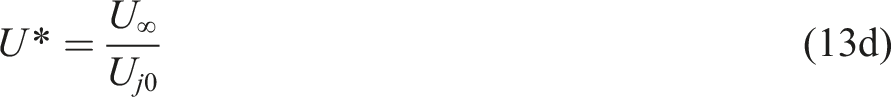
(- 1 + δ) \frac{d I_{m} (\frac{1}{δ} - 1)}{d r} \frac{d K_{m} (\frac{α^{*}}{δ})}{d r} R (δ (4 + δ) S^{2} + ({α^{*}}^{2} {(- 1 + \frac{ω^{*}}{α^{*}})}^{2} - 4 S^{2}) (\ln (R) - \ln (R - δ R))) - {α^{*}}^{2} ({(- 1 + \frac{ω^{*}}{α^{*}})}^{2} I_{m} (\frac{1}{δ} - 1) \frac{d K_{m} (\frac{α^{*}}{δ})}{d r} + (- 1 + δ) \frac{d I_{m} (\frac{1}{δ} - 1)}{d r} K_{m} (\frac{α^{*}}{δ}) {(\frac{ω^{*}}{α^{*}} - U^{*})}^{2}) = 0

(12)

The superscript * denotes non-dimensional parameters, and

δ

is the shear layer thickness.

α^{*} = α (R - R_{0})

(13a)

ω^{*} = ω \frac{(R - R_{0})}{U_{j 0}}

(13b)

S = Ω \frac{(R - R_{0})}{U_{j 0}}

(13c)

U^{*} = \frac{U_{\infty}}{U_{j 0}}

(13d)

δ = \frac{(R - R_{0})}{R}

(13e)

c^{*} = \frac{c}{U_{j 0}} = \frac{ω^{*}}{α^{*}}

(13f)

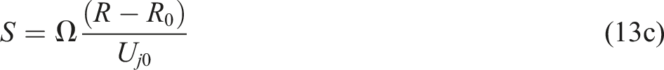
Flow is deemed to be spatially unstable when $α_{i} < 0$ , where the disturbances grow exponentially. A MATLAB program was developed to solve equations (12) and (13a, 13b, 13c, 13d, 13e and 13f) numerically by using “vpasolve” command, and Newton’s method is used with a precision of 32 significant figures.

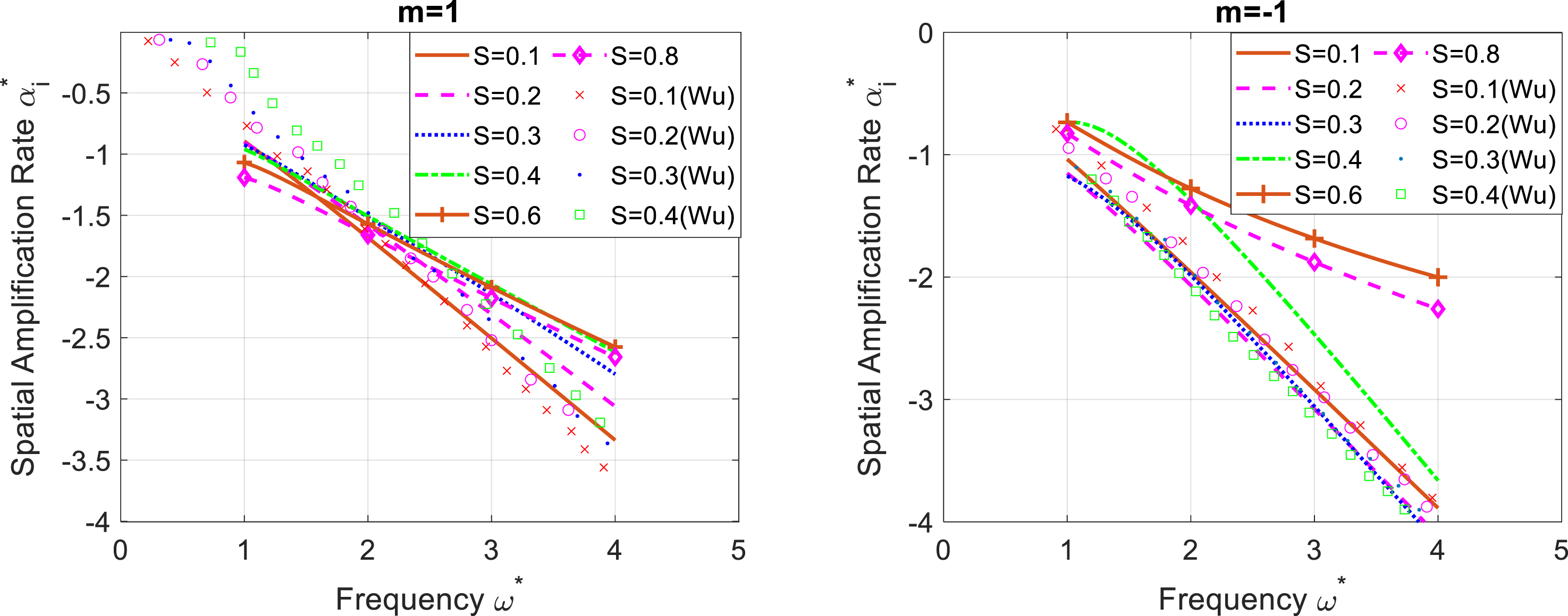
Figure 3 is the spatial amplification rate $α_{i}$ from an inviscid, locally parallel jet with embedded thin-layer swirl, evaluated for the helical modes m = ±1 over swirl parameter S = 0.1-0.8. Across a broad frequency range, the results are compared with inviscid swirling jets from Wu.²² For weak swirl (S = 0.1-0.3) and $ω^{*}$ = 1-4 both the trends and magnitudes of $α_{i}$ closely follow Wu’s data, indicating that the solver captures the essential spatial instability characteristics in this regime. At stronger swirl (S = 0.4), some deviations appear: the current result yields smaller growth for both co-rotating m = +1 branch and counter-rotating m = −1 branch. As discussed earlier, the shifts are consistent with sensitivities to the base flowfield. The influence of the velocity profile increases with swirl intensity. Despite these high-swirl deviations, the overall agreement at low–moderate S supports the validity of the present inviscid Linear Spatial Analysis as a baseline for thin-shear swirling jets.

Figure 3.

Spatial amplification rate $α_{i}$ for inviscid parallel flow with embedded swirl, helical instability wave of m = ±1, swirl parameter S = 0.1-0.8, and comparison with spatial amplification rate for inviscid swirling jets by Wu^22,27.

Figure 4 compares the spatial amplification rate $α_{i}$ for azimuthal modes m = 0, ±1, ±2, ±3 at a fixed swirl level. For weak-to-moderate swirl (S <0.4), the co-rotating branch (m > 0) shows a monotonic increase of | $α_{i} |$ with m, whereas the counter-rotating branch (m < 0) weakens as |m| increases. For a given |m|, the counter-rotating mode is more unstable than its co-rotating counterpart. For weak swirl (S = 0.1), the axisymmetric (m = 0) and helical modes exhibit similar trends of amplification rate which is consistent with Wu. For stronger swirl (S >0.4), the helical modes become frequency dependent: at low frequency ( $ω^{*}$ <2) the counter-rotating modes dominate, with m = −3 amplifies most among the cases examined, whereas at higher frequency ( $ω^{*}$ >2) the trend reverses and the co-rotating modes become more unstable.

Figure 4.

Spatial amplification rate $α_{i}$ of inviscid parallel flow with embedded swirl versus frequency $ω^{*}$ , helical instability wave of m = 0, ±1, ±2, ±3, swirl parameter S = 0.1-0.8, $δ$ = 0.1 and $U^{*}$ = 0.²⁷

Nozzle geometry

The baseline configuration is a round jet with exit diameter D = 0.02,286 m (plain jet). A small swirl vane insert (model m0) is mounted near the exit of the convergent nozzle to generate controlled swirl while keeping the core geometry nearly unchanged. The double-circular-arc airfoil is used in the design of the vanes to generate thin-layer swirl. The thin-layer swirl design uses 12 vanes of 6 mm cord length, the maximum thickness of the vane is 0.762 mm, and is set at 40

°

exit angle, producing swirl number S = 0.09, and the geometry of the baseline nozzle is summarized in Table 1. The swirl number S is defined as the ratio of angular momentum to axial momentum times jet radius R:

S = \frac{\int_{A} r U W d A}{R \int_{A} U^{2} d A} = \frac{\int_{0}^{R} ρ U W r^{2} d r}{R \int_{0}^{R} ρ U^{2} r d r}

(14)

Table 1.

Geometry of the baseline nozzle of 40 $°$ exit swirl angle.

Vane exit angle, deg	Chord length c, mm	Solidity	Number of vanes	Height h, mm	Aspect ratio
40	6	1	12	2.286 (10% D)	0.38

To study the effects of azimuthal swirl modulation on the jet development, three additional nozzle configurations were designed based on model m0, cases m1, m2, and m3. Controlled azimuthal swirl variations in the shear layer are introduced by circumferentially varying the vane angles as a function of the azimuthal angle. It is designed to produce small perturbations (around the 40° mean) and alter the swirl distribution around the circumference near nozzle exit. The variation in the turning angle varies between 0 $°$ and 4.8 $°$ . Cases m = 1, 2, and 3 generate 1-lobe, 2-lobe, and 3-lobe swirl modulation around the nozzle exit, respectively, as shown in Figure 5.

Figure 5.

Exit swirl angle variation with swirl modulation, cases m1, m2, and m3.

Numerical simulation

The Navier-Stokes equations are solved by using large-eddy simulation (LES) in HpMusic solver that based on Flux reconstruction or correction procedure via reconstruction (FR/CPR) method. Spatial discretization employs polynomial degree p = 2. Inviscid fluxes are computed with the Roe approximate Riemann solver and viscous terms are discretized with an interior-penalty (IP) formulation. Subgrid-scale stresses are modeled using the Vreman eddy-viscosity model as implemented in the HpMusic solver.²³ The calibration of the Vreman model was performed using the DNS data of a fully developed turbulent channel flow²⁴ by revising the definition of the filter width:

Δ = \frac{V^{1 / 3}}{\sqrt{p + 1}}

(15)

where V is the volume of the element. Each case is run for 300T_u to ensure enough time for reaching converged state, where T_u is defined as:

T_{u} = D_{e} / U_{j}

(16)

Simulations were conducted for five cases: plain nozzle without vanes and nozzle with thin-layer swirl (model m0, m1, m2, m3). The geometry and the computational domains are shown in Figure 6. The baseline case (plain jet) uses approximately 1.0 $\times 10^{6}$ control volumes. A fully hexahedral mesh is employed for the plain nozzle, whereas a hybrid mesh is used for the swirl-vane model. The domain extends 60 D_e downstream of the exit, with radial extends of 14.5 D_e at the inlet and 29.5 D_e at the outer farfield boundary, where D_e is the nozzle exit diameter. The computational mesh is gradually coarsened near the farfield and exit boundaries to provide damping for possible reflected waves. At the internal nozzle inlet, a subsonic in-flow boundary condition is imposed with a total pressure of 104,191 Pa and total temperature of 290.5 K, which yields a Mach number of 0.2. The upstream and outer radial boundaries are treated as a farfield condition using ambient flow properties (ambient air density $ρ_{\infty} = 1.225 k g / m^{3}$ and pressure $p_{\infty} =$ 101,325 Pa) and a very weak co-flow velocity $U_{\infty} = 0.34 m / s$ , corresponding to approximately 0.1% of the ambient speed of sound. This small co-flow serves to regularize the acoustic radiation at the outer boundary and has negligible influence on the jet development. The downstream boundary at x = 60 $D_{e}$ uses a fixed-pressure subsonic outflow with p = 101,325 Pa, allowing the velocity fluctuations to convect out of the domain. The nozzle and the vane walls are treated using a wall-modeled LES approach, which captures the near-wall turbulence behavior without explicitly resolving the small near wall eddies.

Figure 6.

Flowfield geometry and computational domain in near field of the baseline nozzle.

For wall-modeled LES, the crucial requirement is that the wall model data points should be located within the turbulent boundary layer. Depending on the Reynolds number, the y + can be much higher than 1 since the wall eddies are not resolved. Right near the nozzle exit, the hexahedral mesh is refined to resolve the initial shear layer and the swirling annulus. The x+, y+, and z + are on the order of ∼10. At the nozzle lip, the streamwise and radial grid spacing are $Δ x = Δ r = 0.018 D_{e}$ , and the azimuthal spacing is $Δ r θ = 0.027 D_{e},$ giving 117 cells around the circumference at the nozzle exit. The vane region (swirling annulus block) is discretized using an unstructured isotropic tetrahedral mesh consisting of approximately 3.6 $\times 10^{5}$ tetrahedral cells and a small number of pyramidal elements used to transition to the downstream structured hexahedral mesh. This unstructured block provides the geometric flexibility required to resolve the vane surfaces, while maintaining smooth topological connectivity to the structured region immediately downstream of the nozzle exit. The swirling annulus of thickness is 10% $D_{e}$ and was resolved with eight cells radially. The radial grid spacing of the vane is coarser in the middle and finer near the leading and trailing edges, which is $Δ r =$ 0.0056 $D_{e}$ . Since the flow near the vane changes significantly, the maximum x+, y+ and z+ is on the order of ∼50.

Figure 7 shows a schematic drawing of the conical nozzle. Since the streamlines continue to converge beyond the nozzle geometric exit, the jet forms a virtual throat near the exit. Owing to the streamline curvature, the static pressure at the exit is slightly above the ambient and reaches the ambient at the virtual throat. We therefore treat the virtual throat as the effective jet origin for the free jet and compare axial velocities from that location to ensure consistency with the reference nozzles.

Figure 7.

Schematic drawing of a conical nozzle and its exit flow characteristics.²⁷

A P-refinement study was performed to assess solution independence with respect to polynomial order. Figure 8(a) shows the nondimensional centerline velocity $U^{*} / U_{j}$ versus x/D with the measurements of Quinn,²⁵ and Gilchrist & Naughton.²⁶ HpMusic solver supports polynomial orders p = 0-5 (first to sixth order of accuracy). Results obtained with p = 2 and p = 3 are essentially indistinguishable across the domain, whereas lower orders show small deviations near the potential-core region. Based on this, p = 2 is adopted for all simulations as it provides sufficient accuracy at reduced computational cost.²⁷

Figure 8.

Normalized axial and tangential velocity profiles.²⁷

Figure 8(b) compares the exit plane tangential velocity profiles $V_{θ} (r)$ for the swirling-vane configuration with the reference experimental data from Taghavi, Farokhi and Rice.^28–30 In the present design, the vanes introduce swirl primarily in an outer annulus: $V_{θ} \approx 0$ for r/D <0.3, followed by a sharp rise approaching the nozzle lip. By contrast, the bulk-swirl reference jets exhibit a gradual increase in $V_{θ}$ from the centerline to the outer radius. This exit condition confirms that the current nozzle generates a thin-layer swirl localized near the edge with minimal disturbance to the core flow. Concentrating swirl in the shear layer focuses mixing near the lip and, in principle, limits penalties to core momentum, and thus potential thrust loss.

Farfield sound was reconstructed using a Ffowcs Williams–Hawkings (FWH) formulation on cone-like control surface coaxial with the jet as shown in Figure 9. At the geometric exit plane, the surface radius is 4.8 D from the nozzle lip and then expands downstream to enclose the hydrodynamic source region. FFT size N = 2048, and Hann window was used of duration 0.0333 in solver time units with 50% overlap. The reference pressure $p_{r e f} = 20 μ P a$ , and SPL is:

S P L = 10 \log_{10} (\frac{P}{P_{r e f}})

(17)

Figure 9.

FWH control surface for the round jet.

Results and discussion

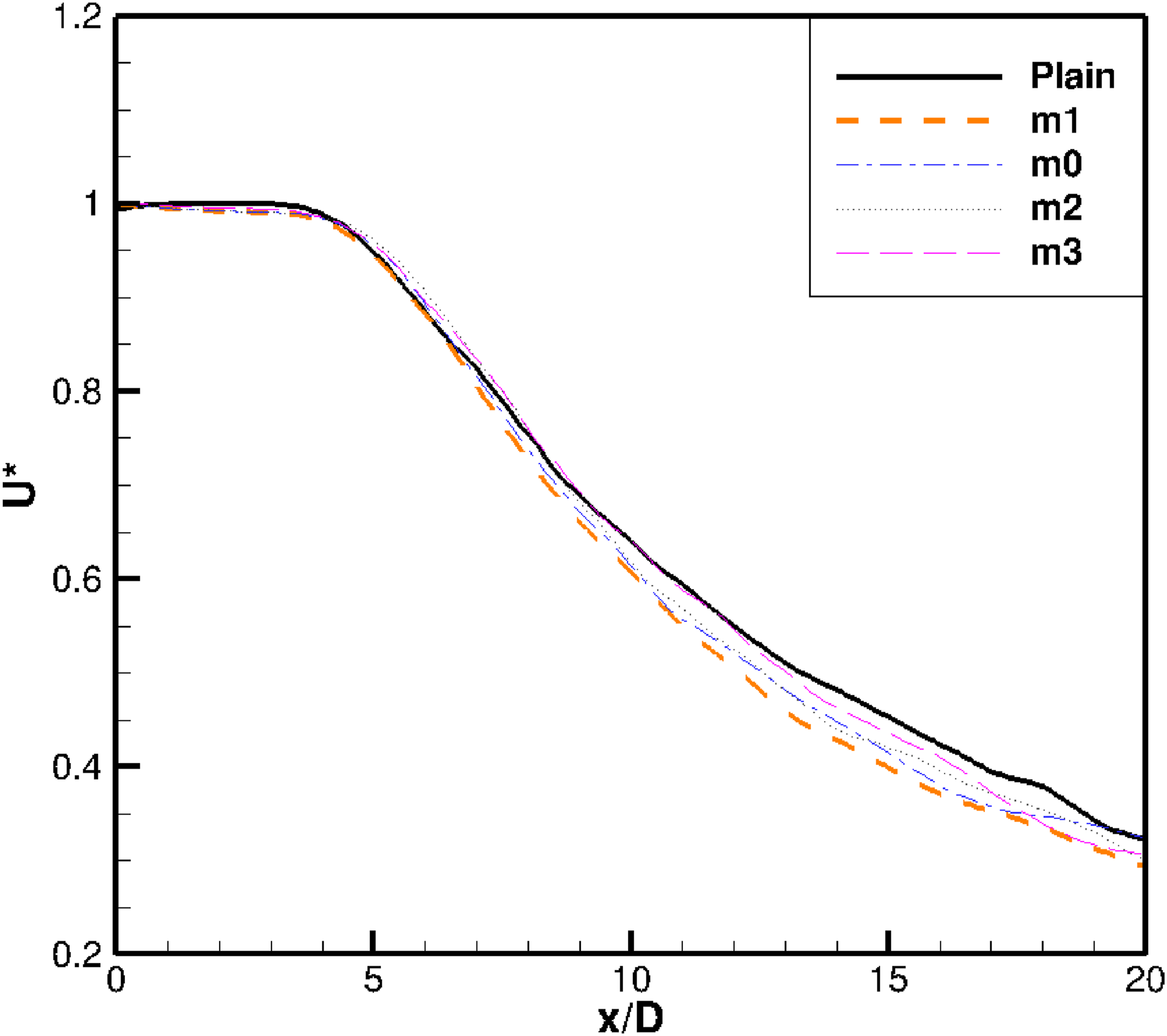
Figure 10 shows the normalized axial velocity ( $U^{*} = U / U_{0})$ along the jet centerline for plain and thin-layer swirling jets. All cases exhibit a finite potential core followed by a monotonic decay consistent with self-similar round-jet behavior. The length of the potential core is approximately 4D for the plain jet and 5D for the swirl cases. Beyond x/D = 6, the decay is approximately linear and the swirl cases show a slightly faster decay in this region, indicating enhanced mixing.

Figure 10.

Normalized centerline axial velocity $(U^{*} = U / U_{0})$ versus x/D for plain and thin-layer swirl cases.

The time-averaged axial velocity contour is plotted in Figure 11, which shows the high-speed potential core and the radial growth of the shear layer. Compared to the plain jet, the swirl configuration exhibits subtle lip-region features that was contributed by the vane wake flow and a slightly earlier onset of shear-layer thickening. Together with the centerline trends, the mean velocity field confirm that the thin-layer swirl primarily acts in the outer annulus near nozzle exit, with an early spreading without strongly affecting the core.

Figure 11.

Mean axial-velocity contours for plain and thin-layer round swirl jets.

Figure 12 presents time-averaged contours of the tangential velocity at the geometric nozzle exit plane for four swirl-vane configurations (cases m0-m3). The swirl is confined to a thin outer annulus for all configurations ( $0.35 \leq r / D \leq 0.55$ ) and the core region remains nearly swirl-free, which is consistent with the thin-layer concept. Maximum value occurs immediately downstream of the vane trailing edges and forms a ring area of high |V|. The unmodulated swirl case (m0) shows an azimuthally uniform ring of V, whereas the azimuthal modulation cases show non-uniform characteristics, as expected.

Figure 12.

Time-averaged tangential velocity V at the nozzle exit plane for cases m0 to m3.

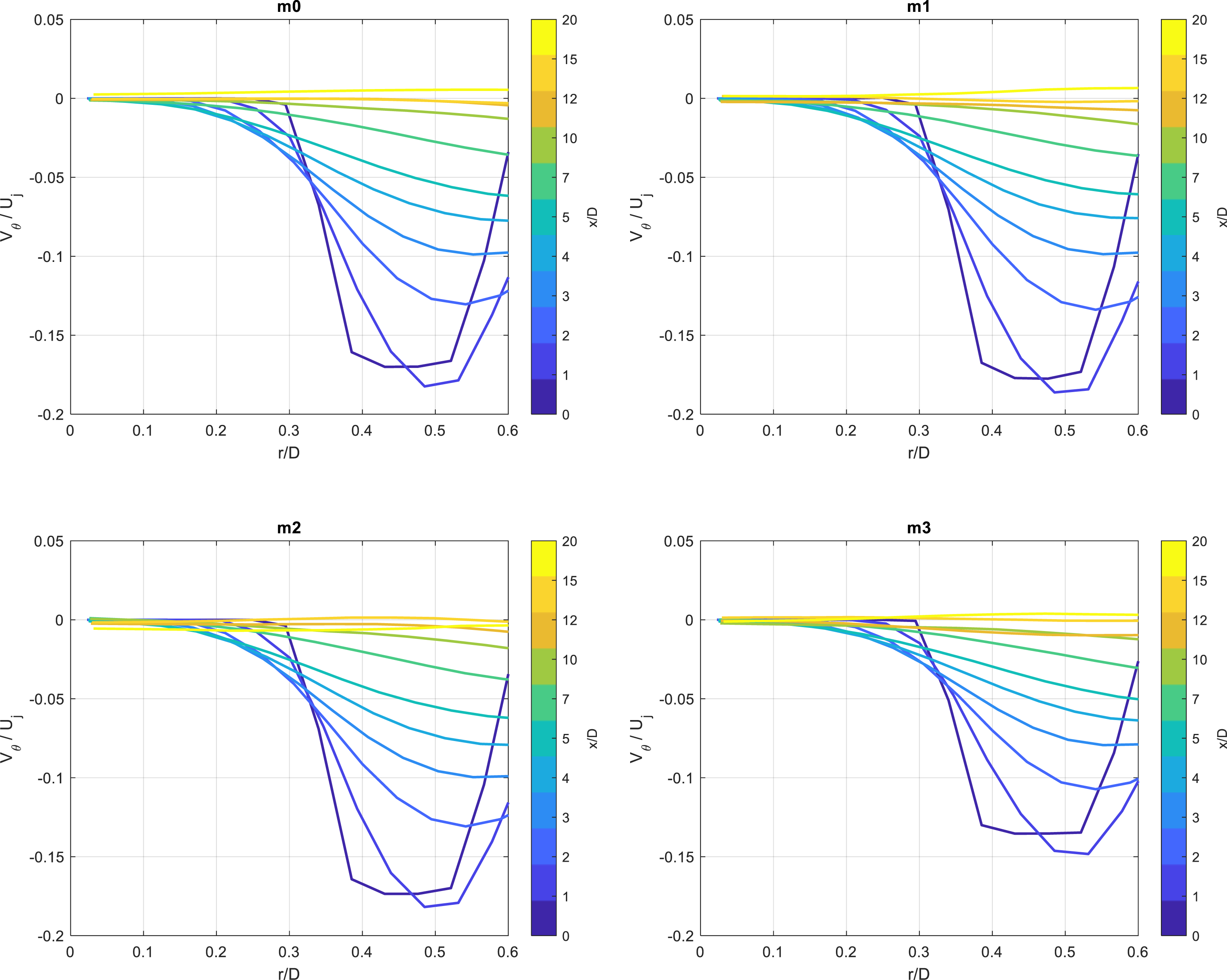
The swirl number S is defined as the ratio of angular momentum to axial momentum times jet radius R, and the swirl number S at the nozzle exit is 0.09. Figure 13 shows the azimuthal velocity profiles $V_{θ} / U_{j}$ at several stations downstream (x/D = 0-20) for the swirling vane configurations (case m0 – m3). At the exit (x/D = 0), the tangential velocity is approximately zero for r/D <0.3 and it shows a sharp increase near the lip which indicates the swirl is confined to an outer radius. The jet continues to contract after the nozzle lip and forms a virtual throat near x/D = 1. The swirling jet develops downstream into a narrower cross-section, the axial flux of angular momentum is conserved without external torque. Therefore, the azimuthal velocity increases with the reduced effective radius which cause the peak tangential velocity near x/D = 1. With increasing x/D, the magnitude of the swirl decays. When x/D approaching 10, the swirl profile is nearly flat. At the virtual throat, where the peak magnitude of swirl is observed, it shows that the case m0 and m2 has slightly higher value compared to m1 and m3, while the downstream decay rate appears similar across designs. Overall, the swirl profiles demonstrate that the swirl vane configurations deliver the intended thin-layer swirl that concentrated near the lip without effecting the core, and further the azimuthal momentum is redistributed through mixing.

Figure 13.

Normalized tangential velocity profiles $V_{θ} / U_{j}$ versus r/D at x/D = 0,1,2,3,4,5,7,10,12,15,20.

The mass flow rate $\dot{m} (x)$ was calculated by the radial-velocity method from Coghe.³¹ At each axial station x/D, the ring-averaged fields in cylindrical coordinates were computed from LES results. An outer integration radius is chosen where the jet approaches the ambient flow ( $\frac{u}{U_{c}} < 0.05$ ). The mass flow rate is then calculated according to:

\dot{m} (x) = 2 π ρ Δ x \sum r_{i} V_{i}

(18)

where

Δ x

is the spacing between the axial locations, and

r_{i}

is selected at the minimum radial distance where

r V = c o n s t

is used in continuity equation. Figure 14(a) shows the mass flow rate normalized by the exit value,

\dot{m} (x) / \dot{m} (0)

and compared with reference data of Coghe of S = 0 and 0.37. The swirl-vane cases display a slightly larger mass flow rate than the plain jet in the near field where x/D <5. All cases exhibit a nearly linear increase for x/D >5. The five configurations stay within ±5% of each other over the entire range. The corresponding (dimensional) entrainment rate,

d \dot{m} / d x

is shown in Figure 14(b). All cases show a rapid increase over near the nozzle exit and reach a maximum value near x/D

\approx

10. The thin-layer swirl jet has a peak value of 0.27

k g s^{- 1} m^{- 1}

, while the plane jet peak is slightly lower with 0.24

k g s^{- 1} m^{- 1}

. This indicates a modest enhancement of entrainment rate due to thin-layer swirl.

Figure 14.

Normalized mass flow rate $\dot{m} (x) / \dot{m} (0)$ and entrainment rate for plain and swirl-vane cases (Coghe 2012 for S = 0 and S = 0.37).

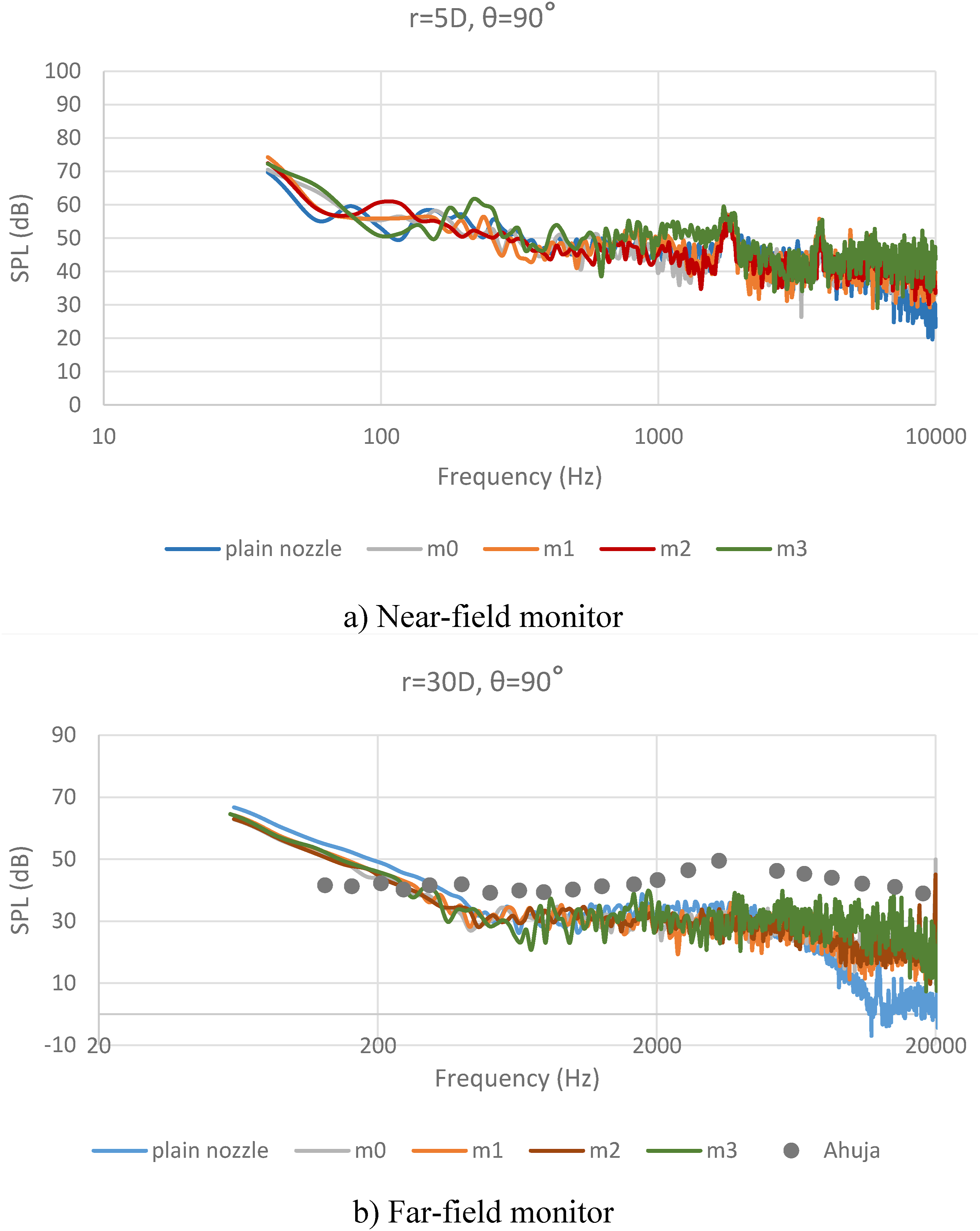
Figure 15(a) shows SPL spectra of five cases at an observation point in the near field with radial distance of 5D and 90 $°$ away from the center of the nozzle exit. All jets follow the expected broadband decay with frequency. In the low–mid frequency range, the five configurations show similar spectra and plain nozzle has slightly lower SPL. In the middle frequency range, case m0, m1, and m2 shows slight noise reduction compared to the plain jet, while some level increase is observed in the high frequency range. At the farfield observation point where r = 30D, the swirl cases (m0–m3) exhibit a low-mid frequency noise reduction compared to the plain jet, while an increase is observed at high frequency. The simulation results are compared with the experimental data from Ahuja,³² and it shows similar slope and trend in the mixing-noise range. Overall, the data indicate that thin-layer swirling jet produces a modest noise attenuation over a broad frequency range. The acoustic validation presented in this study is primarily focused on the comparison of the effects of azimuthal swirl modulation rather than the absolute SPL magnitude. The reference data in Ahuja (1973)³² are obtained from experimental measurements, whereas the present results are based on LES and FWH-based acoustic prediction. Therefore, exact agreement in absolute SPL levels is not expected. The consistency in spectral slope and overall distribution confirms that the simulated flow reproduces essential features. The increase in high-frequency noise observed in all swirling cases is attributed to the enhanced small-scale turbulence generated by the embedded azimuthal velocity gradients. The introduction of swirl promotes the formation of finer turbulent structures, which contribute to the high-frequency acoustic spectrum. In addition, the presence of azimuthal shear introduces additional instability modes that do not exist in the non-swirling jet. From a practical perspective, this result highlights a design trade-off: while thin-layer swirl can enhance mixing and modify large-scale structures that influence low-frequency noise, excessive swirl may shift acoustic energy toward higher frequencies. These findings emphasize the need for optimized swirl strength in noise-control applications to balance mixing enhancement and acoustic performance.

Figure 15.

SPL at near- and far-field location at angle of 90 $°$ with r = 5D and 30D.

The overall sound pressure level (OASPL) at the farfield location where r = 30D is presented in Table 2. It shows a consistent reduction for the thin-layer swirl jet compared to the plain nozzle at both sideline and 60

°

angle. At θ = 90

°

, the plain jet measures 74.0 dB; the vane cases range 70.2–71.9 dB, corresponding to

Δ

OASPL = −2.1 to −3.8 dB, with the highest reduction of −3.8 dB from case m0. At θ = 60

°

, the plain jet is 76.8 dB and the thin-layer swirling jet produces 72.7–73.8 dB, corresponding to

Δ

OASPL = −3.0 to −4.1, with the highest reduction of −4.1 dB from the case m0.

Table 2.

Far-field OASPL at r = 30D for θ = 90 $°$ and 60 $°$ .

Case	OASPL at θ = 90 $°$ (dB)	$Δ$ OASPL vs plain jet (dB)	OASPL at θ = 60 deg $°$ (dB)	$Δ$ OASPL vs plain jet (dB)
Plain	74	–	76.8	–
m0	70.2	−3.8	72.7	−4.1
m1	71.3	−2.7	73.4	−3.4
m2	70.3	−3.7	73	−3.8
m3	71.9	−2.1	73.8	−3.0

The thrust force was obtained at the exit plane from the time-averaged LES results with:

F = \int_{A} [ρ V_{x}^{2} + (p - p_{\infty})] d A

(19)

Where A is the exit area,

V_{x}

is the mean axial velocity,

ρ

is density, and

p_{\infty}

is the ambient pressure. Figure 16 summarizes the thrust penalty relative to the plain nozzle. All swirl vane configurations incur a penalty about 7-9% for case m0-m2 and 11% for case m3. The penalty arises from two mechanisms: (a) momentum redirection from axial to direction; and (b) the swirl vane drags. For additional details on numerical simulation, see Zhao et al.²⁷

Figure 16.

Comparison of the thrust penalty between the plain jet and swirl vane cases. Bars: Thrust difference (N), Dashed line: Percentage loss (%).

The observed thrust penalty results from a combination of axial-to-azimuthal momentum redirection and the profile drag associated with the vane geometry. To separate the “inevitable” penalty due to axial–azimuthal momentum redirection from additional geometric losses, an idealized thin-layer model can be considered. The momentum thrust will be changed with swirling vanes of 40 $°$ exit angle and 10% D height. Assume the original jet velocity (no swirl) is $U$ in the axial direction. With the swirl vanes, part of the flow is turned by 40 $°$ . By assuming the effective exit area of the vaned nozzle remains unchanged due to small vane height and sharp trailing edge, the axial velocity component, in the vaned zone, becomes: $U_{x} \approx U c o s θ$ , and the azimuthal velocity component becomes $U_{θ} \approx U s i n θ$ . Original axial momentum (per unit area) is $ρ U^{2}$ , while the new axial momentum is $ρ {(U c o s θ)}^{2} = ρ U^{2} \cos^{2} θ$ . Therefore, the fraction of axial momentum lost in the pure turning case is ∼ $(1 - \cos^{2} θ)$ . The swirl vanes affect the outer annulus from $\frac{r}{R} = 0.9$ to 1. The annulus area fraction is thus $\frac{A_{s w i r l}}{A_{t o t a l}} = 0.19$ . In the ideal case, 19% of the outer rim of the jet flow is turned by 40 $°$ , which means 81% of the flow is still unaffected by swirl. Therefore, the resulting thrust penalty (in percent) due to flow redirection is estimated as:

Δ F \approx 1 - [1 - \frac{A_{s w i r l}}{A_{t o t a l}} (1 - \cos^{2} θ)] \approx 7.8 %

(20)

This indicates that about 7-8% baseline thrust penalty may be attributed to the flow redirection, i.e., the vane geometry with the aggressive exit flow angle of 40 $°$ (in our case study). The remaining loss of thrust is attributed to the vane profile drag. This implies that a non-negligible portion of the reported 7–11% momentum thrust penalty is due to flow redirection. However, the vane shape, i.e., the mean camber line (MCL), thickness distribution, the vane solidity, the vane aspect ratio, and the vane leading and trailing edge shapes contribute ∼ 3-4% to the thrust penalty. Therefore, future research shall consider a reduction in the vane exit swirl angle as well as the vane shape optimization.

Most of the thrust loss arises from the intended axial-to-azimuthal momentum redirection, while the additional penalty, i.e., beyond ∼7%, is attributed to the vane profile drag. Swirl modulation cases, m1-m3, are found to be less effective in jet noise mitigation as compared to the uniform swirl case, m0. The mechanism may be due to an azimuthally periodic reduced-strength vorticity that swirl modulation creates. The pockets of smaller swirl, contain weaker centrifugal instability that seems to dominate the swirling jet development. Although the jet spreading, characterized by enhanced entrainment rate, affects the reduction in jet noise, the designers should be mindful of thrust loss. Guided by this principle, the thin-layer swirl is confined to the nozzle rim, in the present study. Within this constrained design space, the jet entrainment rate is modestly increased, by 8-17% in the farfield, and by ∼ 21% in the near field (x/D = 0-2), as compared to the plain convergent nozzle. The penalty for thrust loss, i.e., 7-11%, is deemed too excessive. Therefore, the strategy to achieve acceptable noise mitigation (of ∼3 dB) while incurring <5% thrust loss shall include the following design parameters:

(a) The thin-layer swirl fraction extent at the nozzle rim (in the present study 10%)

(b) Exit angle of the swirl vane (in the present study 40 $°$ )

(d) Swirl vane cascade parameters such as solidity and aspect ratio

Conclusion

The thin-layer swirl is introduced by inserting (low aspect ratio) swirl vanes near the lip of a convergent nozzle for mixing enhancement and noise reduction. The instability of the small disturbances was examined by the spatial linear stability analysis. The time-averaged flow field and noise spectra for the low-speed subsonic plain jet and swirl-vane cases were computed by LES. Theoretical analysis of small-amplitude instability waves shows a clear dependence on swirl strength. For weak-to-moderate swirl, the spatial amplification rate increases for the positive helical mode and decreases for the negative helical mode |m|. The negative modes (m < 0), i.e., counter-spinning disturbances, are more unstable. At higher swirl levels, the behavior becomes frequency dependent: the negative helical modes remain dominant at low frequencies, whereas the trend reverses and the positive modes become more unstable at higher frequencies.

A family of thin-layer swirl vane nozzles and azimuthal modulation of the exit swirl were designed with a swirl number of S = 0.09. The simulations show that this modulation reshapes the exit tangential velocity profile, and the case m0 exhibits the highest mixing level. This behavior is consistent with the linear spatial stability results. The stability analysis employed in this study is based on inviscid, incompressible, locally parallel flow assumptions and idealized base-flow profiles. It is not expected to provide quantitatively exact predictions for the fully three-dimensional, viscous, weakly compressible turbulent jet resolved in the LES. In particular, the inviscid and locally parallel assumptions tend to simplify flow structures relative to the evolving shear layer in viscous LES simulations. At the present operating condition (M ≈ 0.2), compressibility effects are small, but non-negligible viscous and non-parallel effects. Therefore, the stability analysis is used to identify dominant instability mechanisms, assess relative changes in amplification behavior with thin-layer swirl, and provide physical insight into the trends, rather than for direct quantitative matching of frequencies or growth rates.

The azimuthal motion is confined to an outer radius and peak swirl values occur near the virtual throat at x/D $\approx$ 1. This follows the conservation of angular momentum flux through the contraction after the nozzle exit. Tangential velocity decays as jet develops downstream. The mass flow rate grows nearly linearly for x/D >5 and the entrainment function rise rapidly in the near field and reaches peak values around x/D = 10. The swirl-vane cases show a modest near and farfield entrainment enhancement as compared to the plain jet.

The swirl configurations yield more than 3 dB OASPL reduction at the farfield location of r = 30D at 90 $°$ and 60 $°$ , with case m0 shows strongest effect. Compared to the plain jet, the SPL decrease in the low–mid band, while a modest rise appears at higher frequencies. This pattern is consistent with introducing swirl to the mixing process in the shear layer: From an application standpoint, thin-layer swirl offers a net noise benefit with some level of high-frequency noise increase. It suggests that the future optimization of vane shape, solidity and aspect ratio has the potential to inhibit noise radiation while maintaining <5% thrust penalty. The current swirl vanes, which are not optimized for thrust loss mitigation, incur about 7-11% thrust penalty. We anticipate future design optimizations to reduce thrust loss to an acceptable level of <5%.

Supplemental Material

Supplemental Material - The role of embedded swirl in shear layer on turbulent jet mixing and noise

Supplemental Material for The role of embedded swirl in shear layer on turbulent jet mixing and noise by Lu Zhao, Ray Taghavi, Zhi J. Wang, Saeed Farokhi in International Journal of Aeroacoustics.

Footnotes

ORCID iD

Lu Zhao

Funding

The authors received no financial support for the research, authorship, and/or publication of this article.

Declaration of conflicting interests

The authors declared no potential conflicts of interest with respect to the research, authorship, and/or publication of this article.

Supplemental Material

Supplemental material for this article is available online.

References

Martens

Spyropoulos

. Practical jet noise reduction for tactical aircraft. In: Proceedings of ASME Turbo Expo 2010: Power for Land, Sea and Air. American Society of Mechanical Engineers (ASME), 2010.

Liu

Zhao

Guan

, et al. Development and progress in aeroacoustic noise reduction on turbofan aeroengines. Prog Aero Sci 2022; 130: 100796.

Gorji-Bandpy

Azimi

. Technologies for jet noise reduction in turbofan engines. Aviation 2012; 16(1): 25–32.

Dahl

McDaniel

. The performance of jet noise suppression devices for industrial applications. J Vib Acoust 1985; 107(3): 303–309.

Schwartz

. Jet noise suppression by swirling the jet flow. In: AIAA Aeroacoustics Conference. American Institute of Aeronautics and Astronautics (AIAA), 1973.

Ramsay

Miller

. Noise of swirling exhaust jets. AIAA J 1977; 15(5): 642–646.

Papamoschou

. Fan flow deflection in simulated turbofan exhaust. AIAA J 2006; 44(12): 3088–3097.

Balakrishnan

Srinivasan

. Influence of swirl number on jet noise reduction using flat vane swirlers. Aero Sci Technol 2018; 73: 256–268.

Papamoschou

. New method for jet noise reduction in turbofan engines. AIAA J 2004; 42(11): 2245–2253.

10.

Suzuki

. A review of diagnostic studies on jet-noise sources and generation mechanisms of subsonically convecting jets. Fluid Dyn Res 2010; 42(1): 014001.

11.

Karabasov

. Understanding jet noise. Philos Trans A Math Phys Eng Sci 2010; 368(1924): 3593–3608.

12.

Lighthill

. On sound generated aerodynamically I. General theory. Proceedings of the Royal Society of London. Series A. Mathematical and Physical Sciences 1952; 211(1107): 564–587.

13.

Lighthill

. Jet noise. AIAA J 1963; 1(7): 1507–1517.

14.

Rayleigh

, On the instability of jets. Proc Lond Math Soc 1878; s1-10: 4–13.

15.

Guitton

Kerherve

Jordan

, et al. The sound production mechanism associated with coherent structures in subsonic jets. In: 14th AIAA/CEAS Aeroacoustics Conference (29th AIAA Aeroacoustics Conference), Vancouver, 2008.

16.

Wan

Zhou

Sun

. A study on large coherent structures and noise emission in a turbulent round jet. Sci China Phys Mech Astron 2014; 57(8): 1552–1562.

17.

Michalke

. The instability of free shear layers. Prog Aero Sci 1972; 12: 213–216.

18.

Chan

. Spatial waves in turbulent jets. Phys Fluids 1974; 17(1): 46–53.

19.

. Spatial instability of a swirling flow. Appl Math Mech 1984; 5(2): 1221–1229.

20.

Han

Taghavi

Farokhi

. Passive control of supersonic rectangular jets through boundary layer swirl. Int J Turbo Jet Engines 2013; 30(2): 199–216.

21.

Rahmani

Alhawwary

Wang

, et al. Noise mitigation of a supersonic jet using shear layer swirl. In: AIAA Scitech 2020 Forum, Orlando, FL, USA, 2020.

22.

Farokhi

Taghavi

. Spatial instability of a swirling jet - theory and experiment. AIAA J 1992; 30(6): 1545–1552.

23.

Wang

Jia

, et al. Towards industrial large eddy simulation using the FR/CPR method. Computers & Fluids 2017; 156: 579–589.

24.

Duan

Wang

. Calibrating sub-grid scale models for high-order wall-modeled large eddy simulation. Adv Aerodyn 2024; 6(1): 5.

25.

Quinn

. Measurements in the near flow field of an isosceles triangular turbulent free jet. Exp Fluids 2005; 39: 111–126.

26.

Gilchrist

Naughton

. Experimental study of incompressible jets with different initial swirl distributions: mean results. AIAA J 2005; 43(4): 741–751.

27.

Zhao

Taghavi

Farokhi

, et al. The effect of thin-layer swirl on turbulent jet mixing and noise. In: AIAA Aviation Forum and Ascend. American Institute of Aeronautics and Astronautics (AIAA), 2025, p. 2025.

28.

Taghavi

Rice

Farokhi

. Controlled excitation of a cold turbulent swirling free jet. J Vib Acoust 1988; 110(2): 234–237.

29.

Farokhi

Taghavi

Rice

. Effect of initial swirl distribution on the evolution of a turbulent jet. AIAA J 1989; 27(6): 700–706.

30.

Farokhi

Taghavi

Rice

. Modern developments in shear flow control with swirl. AIAA J 1992; 30(6): 1482–1483.

31.

Recalcati

Cozzi

Coghe

. Measurement of entrainment rate in the initial region of swirling jets. Proceedings of the XXXV Meeting of the Italian Section of the. Combustion Institute, 2012.

32.

Ahuja

Bushell

. An experimental study of subsonic jet noise and comparison with theory. J Sound Vib 1973; 30(3): 317.

Supplementary Material

Please find the following supplemental material available below.

For Open Access articles published under a Creative Commons License, all supplemental material carries the same license as the article it is associated with.

For non-Open Access articles published, all supplemental material carries a non-exclusive license, and permission requests for re-use of supplemental material or any part of supplemental material shall be sent directly to the copyright owner as specified in the copyright notice associated with the article.

0.00 MB

0.30 MB