
Abstract
Coastlines are changing, wildfires are raging, cities are getting hotter, and spatial designers are charged with the task of designing to mitigate these unknowns. This research examines computational digital workflows to understand and alleviate the impacts of climate change on urban landscapes. The methodology includes two separate simulation and visualization workflows. The first workflow uses an animated particle fluid simulator in combination with geographic information systems data, Photoshop software, and three-dimensional modeling and animation software to simulate erosion and sedimentation patterns, coastal inundation, and sea level rise. The second workflow integrates building information modeling data, computational fluid dynamics simulators, and parameters from EnergyPlus and Landsat to produce typologies and strategies for mitigating urban heat island effects. The effectiveness of these workflows is demonstrated by inserting design prototypes into modeled environments to visualize their success or failure. The result of these efforts is a suite of workflows which have the potential to vastly improve the efficacy with which architects and landscape architects use existing data to address the urgency of climate change.
Keywords
Introduction
Climate change predictions create challenges for landscape architects, who typically do not use scientific data to predictively model long-range environmental flux as a design analysis tool. Despite this, landscape architects are well equipped to design for change and uncertainty, and to provide alternatives which may repair or deflect the damage caused by climate-change-related occurrences. In response to these challenges, we look at methods for simulating and visualizing coastal storms and urban heat effects related to climate change. In addition, we explore creating dynamic models which improve the outcomes of these visualizations, essentially using the simulations to test design alternatives and understand their effectiveness. We discuss the development of these computational models showing storms and urban heat islands, as well as the design strategies which we tested and whether they worked. We share the software workflows and scientific data sources used in these studies and will discuss the benefits of implementing these workflows as landscape architecture design and planning tools.
Current landscape architecture digital tools
As climate change becomes an increasingly common aspect of planning and design of urban spaces, landscape architects face challenges of great ecological complexity. Landscape architecture software workflows, already lagging due to slow adoption of Building Information Modeling (BIM), are now further pressured by the demand to use sophisticated software workflows in addressing complex climate change scenarios. 1 These pressures require adaptation of traditional design processes in order to create aspirational designs which can continually cool ever-hotter urban areas as well as tolerate extreme weather events such as coastal storms. 2 This raises the question of what digital techniques landscape architects must assemble in order to accomplish these tasks. Without a single piece of software that can address the full complexity of designing for the landscape, we propose the assembly of several existing digital tools to import scientific climate and environmental data and create simulated three-dimensional (3D) environments for testing design solutions.
Current software workflows for visualizing impacts of climate change do exist, and the urgency of climate change requires that we attempt to model these unknowns as best we can. Landscape architects still use computer-aided design (CAD) software on a daily basis, usually AutoCAD 3 for design development and documentation. They also use geographic information systems (GIS) software to document existing physical and demographic conditions. The common use of GIS software in landscape architecture has broadened the CAD workflow to include geospatial aspects, arguably the strongest “intelligent” tools used by landscape architects, and their interoperability with CAD systems is strong and established. 4 Furthermore, landscape architects also make use of parametric design tools for creating responsive algorithmic design, for instance, the Rhino 5 tool Grasshopper, which is effective at inputting dynamic data and rapidly outputting different spatial forms. For instance, Grasshopper can be used to perform daylighting analysis, commonly used for interior architectural temperature analysis, but also used for exterior conditions. 6 Grasshopper can also be used to generate morphology influenced by repetitive patterning, such as the creation of crystalline and glass-like shapes which respond to numerous parametric inputs, a tactic which we will describe later in this article as a way of creating cooling channels of urban air flow. 7
Environmental solar energy simulations are usually created using standardized weather files which are based on current data and do not take future climate predictions into account. However, climate-change-adapted weather data simulation is possible and has been attempted for several years, with many established methods. One approach is to use available end-user software tools, such as CCWorldWeatherGen 8 and WeatherShift™, 9 to generate future projection weather data that can be used for executing building and environmental performance simulation. However, these tools do not operate similarly and therefore may produce widely varying results. In addition, in the case of WeatherShift™, the software only modifies the most significant meteorological parameters, an aspect that is of major importance in situations when less significant meteorological variables need to be included.10,11 Another approach is to “morph” existing EnergyPlus™ 12 data with UK Met Office Hadley Center general circulation model (GCM) predictions for a “medium–high” emissions scenario (A2). This approach makes use of the existing CCWorldWeatherGen software, placing certain limits on it to eliminate unrealistic results. Although there are some small issues with this workflow, most notably the tendency to underestimate the impacts of climate change, it is considered to be a practical approach to deriving weather files suitable for climate-change impact assessment in the built environment.10,11 A third approach is to synthesize weather data sets out of several climate scenarios, based on 1-year weather data which can be generalized for 30-year periods. This approach produces scientifically valid energy performance assessments while keeping the number of simulations much lower than other methods. 13
Some computational design researchers have begun to address the area of information-driven landscape modeling, developing algorithms that emulate and visualize the behavior of natural systems. The Nature of Code 14 provides a framework for software simulation of natural forces in spatial environments, including gravity, friction, and velocity. Testing the Waters, 15 a project by Peg Office of Landscape Architecture, explores wetland suitability strategies that are directly guided by energy and elevation parameters, modeled using GIS, computational flow dynamics, and parametric software. Work in digitally simulating the flow of rivers has produced valuable ideas regarding the use of robotics to manage sedimentation. 16 Hydrology researchers have long been using computational models to visualize potential loss of coastal cliffs using GIS software, using a virtual reality workflow to communicate these potentials to lay audiences. One example is the Soft Cliff and Platform Erosion (SCAPE) model, 17 which uses GIS and a computational algorithm to visualize future cliff erosion scenarios based on erosion, wind, and sea level rise. The development of Ladybug Tools 18 for Grasshopper has allowed designers to optimize their designs using true environmental data which can be seamlessly input into the 3D model to generate more realistic feedback. 19 The development of these open-source tools has advanced to the point where integration of computational fluid dynamics (CFD) now permits the modeling of air flows within the Grasshopper environment. This is a particularly important development for landscape architects, who rely on accurate modeling of exterior environmental conditions. 20
Methods
The first project we discuss involves digitally simulating coastal conditions using 3D modeling of erosion scenarios and animated visualization of future coastal storm events. The second project involves digitally simulating urban heat island effects using a 3D model, through visualization of surface temperatures based on surface material as well as visualization of sun, shade, and air flow. Although the case studies use two different sites, these two projects can effectively be considered as two arms of an overarching workflow to evaluate and iterate resilient landscape designs. Both can be viewed as frameworks for conducting applied research leading to practice, with methodologies that can be adapted by practitioners to develop and test resilient designs. The tools that are used in these workflows are mostly those used by professional landscape architects, and the stages of analysis and design that are represented mirror the phases of design in practice.
In both cases, we first analyzed current and future conditions of storm inundation and urban heat islands, simulating scenarios where the existing landscape is left to be impacted by coastal change and hotter temperatures. Once these baseline hypothetical conditions were visually realized, we proceeded to test design interventions which were intended to offset the most harmful impacts.
The methods for simulating coastal conditions can be split into three discrete parts:
Simulating erosion with historic erosion rates imposed onto Lidar terrain data using ESRI ArcMap, 21 Adobe Photoshop, 22 the Geographic Imager Photoshop plugin, 23 and Rhino.
Simulating sea level rise using anticipated future rates of sea level rise, using Rhino.
Simulating coastal storms based on National Oceanic and Atmospheric Administration (NOAA) 24 data, using Autodesk Maya. 25
This workflow is shown in Figure 1.
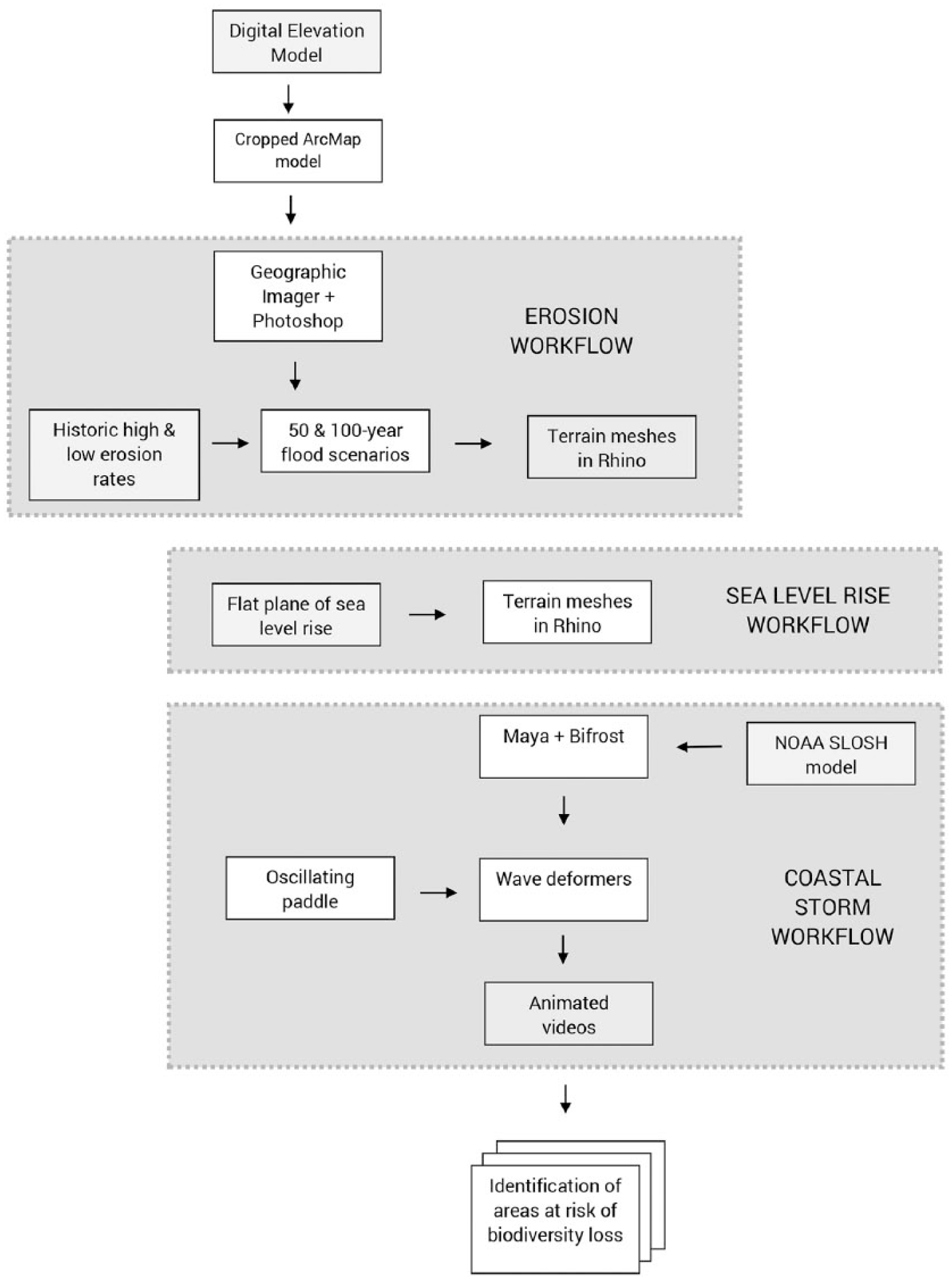
Diagram of erosion, sea level rise, and storm surge digital workflow.
The methods for simulating urban heat island effects can be split into four discrete parts:
Simulating regional heat patterns using Rhino, Grasshopper, Ladybug Tools Dragonfly utility, and the Geographic Imager Photoshop plugin.
Simulating hardscape albedo based on EnergyPlus™ Weather (EPW) material thermal performance data, using Rhino, Grasshopper, and the Ladybug Tools Honeybee utility.
Simulating sun and shade patterns based on historic weather data, using Rhino, Grasshopper, and Ladybug Tools.
Air flow analysis based on historic weather data, using Rhino, Grasshopper, the Ladybug Tools Honeybee utility, and OpenFOAM. 26
This workflow is shown in Figure 2.

Diagram showing hardscape, sun and shade, and air flow analysis workflow.
Case studies
Both case study sites share common traits of being located on the Atlantic coast, in densely populated areas which are subjected to frequent major storm events. For the coastal modeling workflow, we chose Misquamicut Beach in Westerly, Rhode Island, for its relative coastal density for a small town, as well as its function as a partial barrier island. For the urban heat island workflow, we chose the Boston, Massachusetts, neighborhood of Roxbury, for its high level of urban density and lack of open space. These two case study sites are less than 100 miles apart and represent two extremes: one is a major metropolitan center with over 1 million residents and high tourism rates; the other is a small coastal community of less than 25,000 residents and is a popular vacation spot.
Cast study 1: simulating erosion, sea level rise, and storm surge
The main goal of this workflow was to computationally simulate and visualize future conditions of a site undergoing erosion caused by sea level rise, create an animated model of a major coastal storm within these future conditions, and develop a responsive landscape architecture design proposal. In order to meet this goal, we needed to create a digital model that more accurately reflected the interrelated impacts which drive erosion: waves, tides, and changes in sea level rise. 17 One impediment was that the existing tools used to model and predict sea level rise are not dynamic ecological models, and as such are not informed by the adaptive responsiveness of coastal ecologies, ecologies which can often reform and adapt to encroaching water. 27 We aimed to overcome this obstacle using a range of geospatial, image editing, 3D modeling, and animation tools, which enabled us to model the impacts of sea level rise, storm inundation, and erosion as a dynamic, evolving set of relationships.
Out of necessity, we made intentional assumptions. Although it is known that erosion rates change frequently, we were unable to predict how these rates would change in the future. Because of these unknowns, we opted to used fixed values, setting a low erosion rate of 0.2 m/year and a high erosion rate of 0.5 m/year. One important note is that these rates are greater than the average recorded rate in that area since 1939, 28 but are in sync with the rates of sea level rise used in similar digital simulations of coastal erosion in other coastal erosion studies. 29 A second assumption we made was that the case study site was composed of a single site material, eliminating distinctions between hardscape and permeable surfaces. This was necessary to establish areas of control where we could be certain no material differences were contributing to irregularity in the simulations. The importance of modeling differentiated in situ site materials, such as variations in rock strength, permeability, and drag, will be an important component to include in future development of this workflow.
We began the erosion process with a digital elevation model (DEM) from the United States Geological Survey’s (USGS) National Map Viewer. 30 We imported the DEM into in ArcMap GIS software. Once the DEM had been acquired, we needed to computationally erode the coastline at these set rates. We discovered that although the DEM could easily be exported to a 3D modeling software program, the 3D modeling tools did not allow us to methodically reshape the coastline with any geospatial accuracy. Resorting to the accuracy and reliability of two-dimensional (2D) image editing, we opted to work directly with the DEM image file and erode the coastline in the raster image that was used to generate the 3D model. To accomplish this 2D erosion, we used the Geographic Imager plugin, which allowed the spatial properties of the image to be automatically updated and maintained during raster image editing. This allowed us to clone stamp the coastline pixel data further inland at geospatially accurate distances between the sample and paint locations (Figure 3).
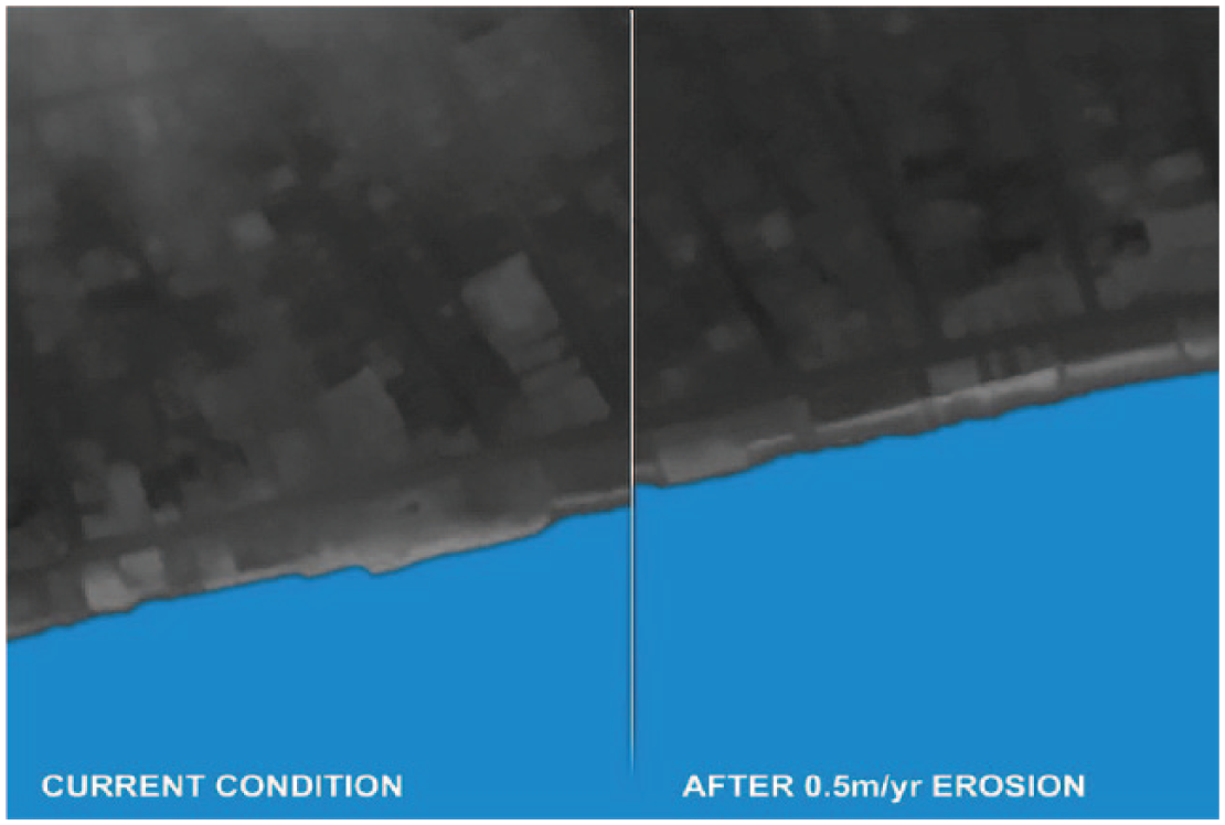
Digital elevation model showing current and eroded conditions.
After creating several modified DEMs representing various erosion scenarios, we exported the DEMs from Geographic Imager and back into ArcMap, where they appeared as a series of layers on top of the original DEM. The modified DEMs were exported as American Standard Code for Information Interchange (ASCII) point data and imported into Rhino as a terrain mesh. We created a flat plane representing a simplified measurement of sea level height above current mean tide, intersecting the planes with the eroded terrain meshes. Sea level heights are projected to increase between 0.8 m and 1.8 m by 2100. We have used these approximations to create three scenarios, with 2 ft of sea level rise being the most conservative risk scenario, 4 ft of sea level rise being an intermediate risk scenario, and 6 ft of sea level rise being the most extreme risk scenario. 31 These visualizations show that ocean inundation combined with shoreline erosion could lead to the breaching of coastal barrier islands and resulting saltwater inundation into freshwater ponds (Figure 4).
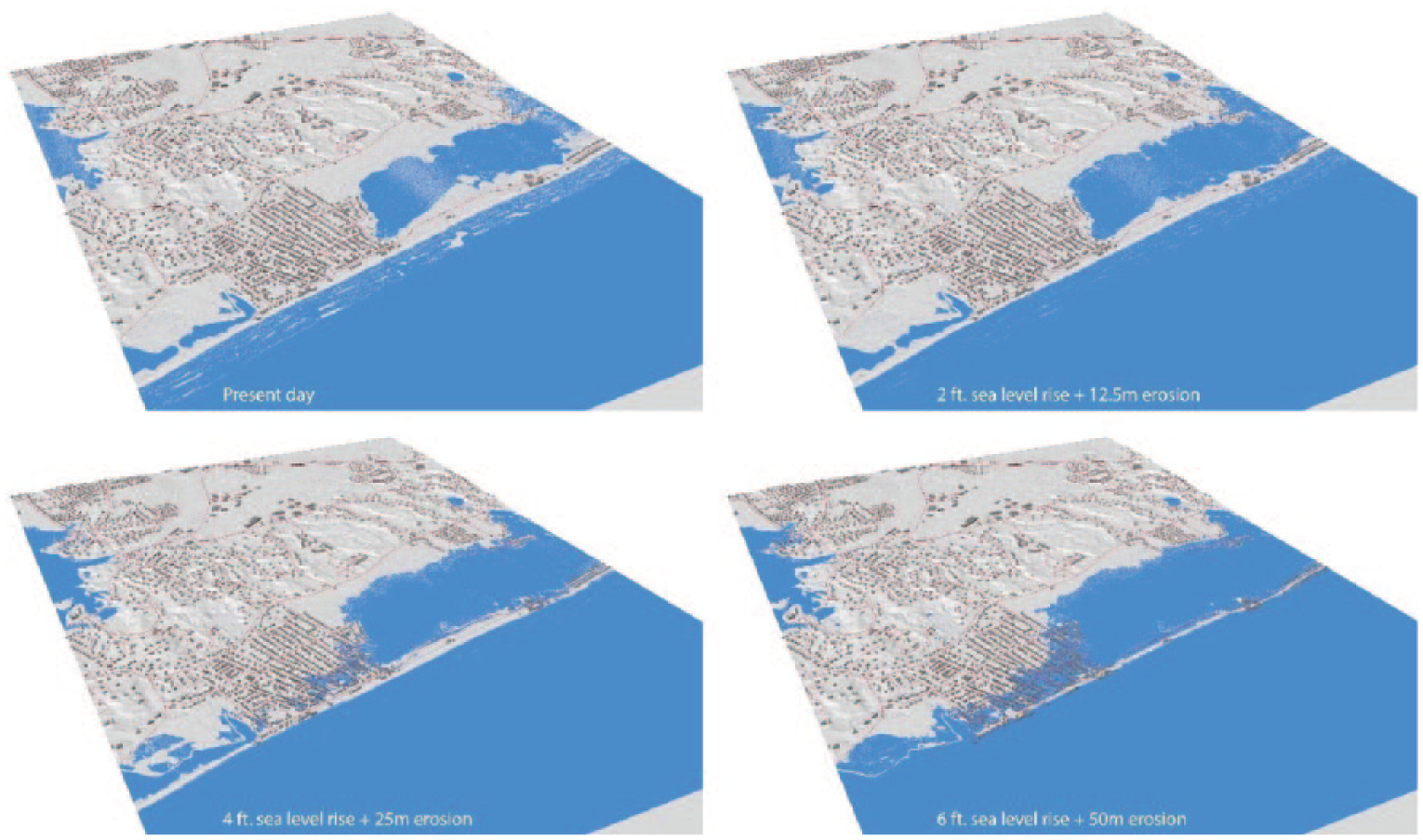
Visualizations showing sea level rise rates coupled with increasing erosion.
Static imagery has some limitations when used to represent dynamic landscape elements. This is especially true when simulating dramatic natural events such as heavy wind and water. To create a more realistic model, our next task was to create an animated simulation of coastal waves. We first identified the potential maximum height of a storm surge in this specific area of the Rhode Island coastline, referencing the Sea, Lake, and Overland Surges from Hurricanes (SLOSH) 32 model from NOAA’s Hurricane Modeling System to provide storm surge ranges for the site’s general vicinity. SLOSH is a computerized model which estimates and visually displays storm surge heights for historical, hypothetical, or predicted hurricanes. These estimates make use of data on atmospheric pressure, size, forward speed, and track data, which are used to create a model of the wind field which generates the storm surge. The SLOSH model is especially useful because it responds to the physical features of a delineated area such as shoreline and inland hydrology, depth, and infrastructure. We used a SLOSH modeling approach called the probabilistic approach, which incorporates statistics of past forecast performances to generate an ensemble of SLOSH runs. 33
Once we had identified the maximum possible storm surge height, we turned our attention to modeling the storm surge water body in motion. Several software tools exist which can animate fluid particles in 3D space. In evaluating the available software, two options emerged, which were useful because they could model fluid particles in 3D space with a high degree of technical accuracy and visual legibility. The first option, RealFlow, 34 offers rigid and soft body dynamics solvers, making it ideal for large-scale simulations such as floods or oceans with breaking waves, as well as small-to-medium ocean surfaces. 35 The second option, Bifrost, a tool within Maya, is a procedural framework that uses a fluid implicit particle solver to create simulated liquid effects. Bifrost also includes an Ocean Simulation System, which can create realistic ocean surfaces with waves, ripples, and wakes. Ultimately, we selected Bifrost because of its seamless integration within the Maya 3D modeling environment, allowing the smoothest exchange of 3D models with other CAD software. Bifrost’s credibility as a hydrological simulation tool comes from its usage of the Navier–Stokes solver to generate fluid particle motion, written here in pressure–velocity variables
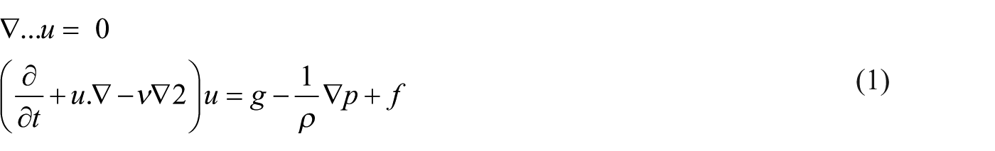
where
The Navier–Stokes equations are commonly used to describe the motion of viscous fluid substances, and their usage for animation and rendering of complex water surfaces allows preservation of much of the realistic behavior of water while also allowing a sufficient degree of control necessary for animation and rendering environments. 36
The first step in modeling the storm surge water body was to import the existing current-day terrain model from Rhino. Because of the computational power required to produce the animations, we divided the site into smaller sections and focused on a single topographic slice. Using a Bifrost simulation at the average height of 11 ft above sea level—that of a category 1 storm surge—we intersected this moving liquid plane with the eroded terrain mesh. To generate further turbulence, we added a cross wave and programmed in periodic fluctuations in the height of the waves. This further amplified the wave action and the distance that the storm surge could travel ashore.
After running initial animations showing a coastal storm surge, our next goal was to apply the wave behavior to an eroded coastline, simulating a future scenario that could occur due to sea level rise. To accomplish this, we imported the edited terrain models and ran animations replacing the existing terrain model with ones showing erosion, factoring in higher wave elevations due to sea level rise. We observed that the tiny remnant of the coastal barrier island is easily breached by storm surge, removing any remaining protection to the heavily populated inland area (Figure 5). Moreover, this complete loss of the barrier island, and the influx of coastal waters, dramatically changes the composition of the adjacent ecosystem.
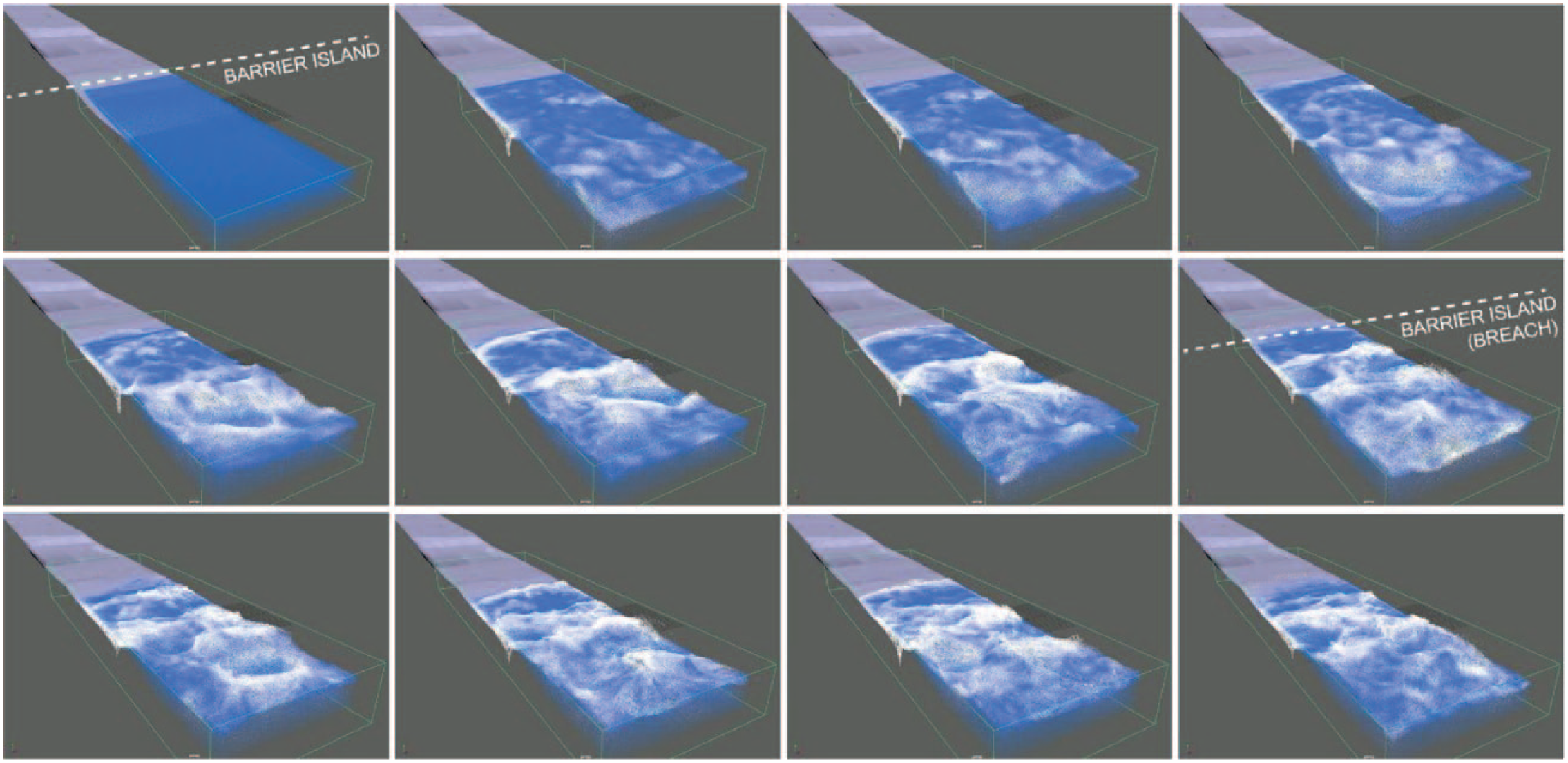
Animation stills showing a category 1 hurricane breaching the eroded barrier island.
Using geospatial data showing ecological zones along the study area, we mapped specific ecological areas onto our simulations. These indicate that the advanced level of shoreline retreat could significantly reduce or eliminate areas of inland swamp, as well as brackish and freshwater marshes. With these losses in mind, we set out to develop a design strategy which would preserve these reduced ecologies through gradual inland relocation. This is an uncommon tactic, as most sea level rise design interventions aim to mitigate damage in situ using barriers to keep water out or inlets to allow water to circulate around built form. In contrast, the design strategy emerging from our research prioritizes the full relocation of major ecological areas, while aiming to have a minimal impact on existing built form. Within the study area, our research indicates that the largest inland water body facing total loss is Winnepaug Pond, a swamp and salt marsh fed by Weekapaug Beachway. Our models show that sea level rise and erosion will eventually convert this water body to coastal beach, a change made even more dramatic due to loss of barrier islands (Figure 6). With this in mind, we ask the radical question: could a landscape design possibly recreate this lost ecology in a nearby inland area?
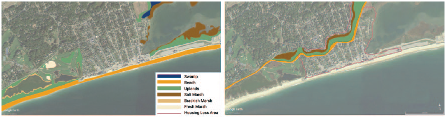
Current and future conditions showing biodiversity loss.
We identified a suitable area to relocate this water body. Our site selection was based on finding an area that was relatively undisturbed by development, large enough in area to accommodate the water volume of Winnepaug Pond, and lower in elevation than the surrounding areas. These criteria led us to select an area of inland mixed forest and swamp which connects to the Newton Swamp Management Area. Although significant further analysis would be necessary to determine real-life site suitability, as an initial proof of concept, this level of analysis is sufficient to model a spatial design strategy.
We located a series of depressed land areas which could gradually be inundated, with connecting channels between each basin. The first identified basin was Doctor Lewis Pond, which is only a few hundred feet from the closest area of predicted inundation from sea level rise, and is separated from the inundation area by a single road. We re-graded the edge of the pond to connect to the edges of Winnepaug Pond, proposing a bridge over the connective inlet (Figure 7). Winnepaug Pond is predicted to become the eventual shoreline edge, and as such this new grading effectively connects the inland basin of Doctor Lewis Pond to the Atlantic Coast. This re-grading allows the flow of coastal water into a larger inland basin, passing underneath a bridge and impacting two structures and a small portion of a road.
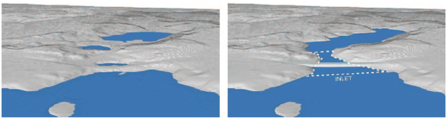
Existing conditions showing inland basin (left) and proposed re-grading to allow ocean water to flow in (right).
We ran this model through our previous Bifrost particle simulator to visualize the possible force of a coastal storm on this reshaped landscape as it flowed through the newly shaped channel into the inland basin. The resulting animation indicates that although the narrow inlet causes extreme turbulence of the moving water, the water does flow primarily into the basin and does not redirect upward to residential areas. One benefit of this level of turbulence at the inlet is that the slowing of this water will reduce inland erosion. Yet, a critical drawback is that it could likely erode the inlet shoreline—already quite steep due to re-grading—causing harmful levels of erosion. This is a drawback that will need to be explored further, perhaps testing methods of slowing down the water through smaller estuaries or widening the inlet (Figure 8).
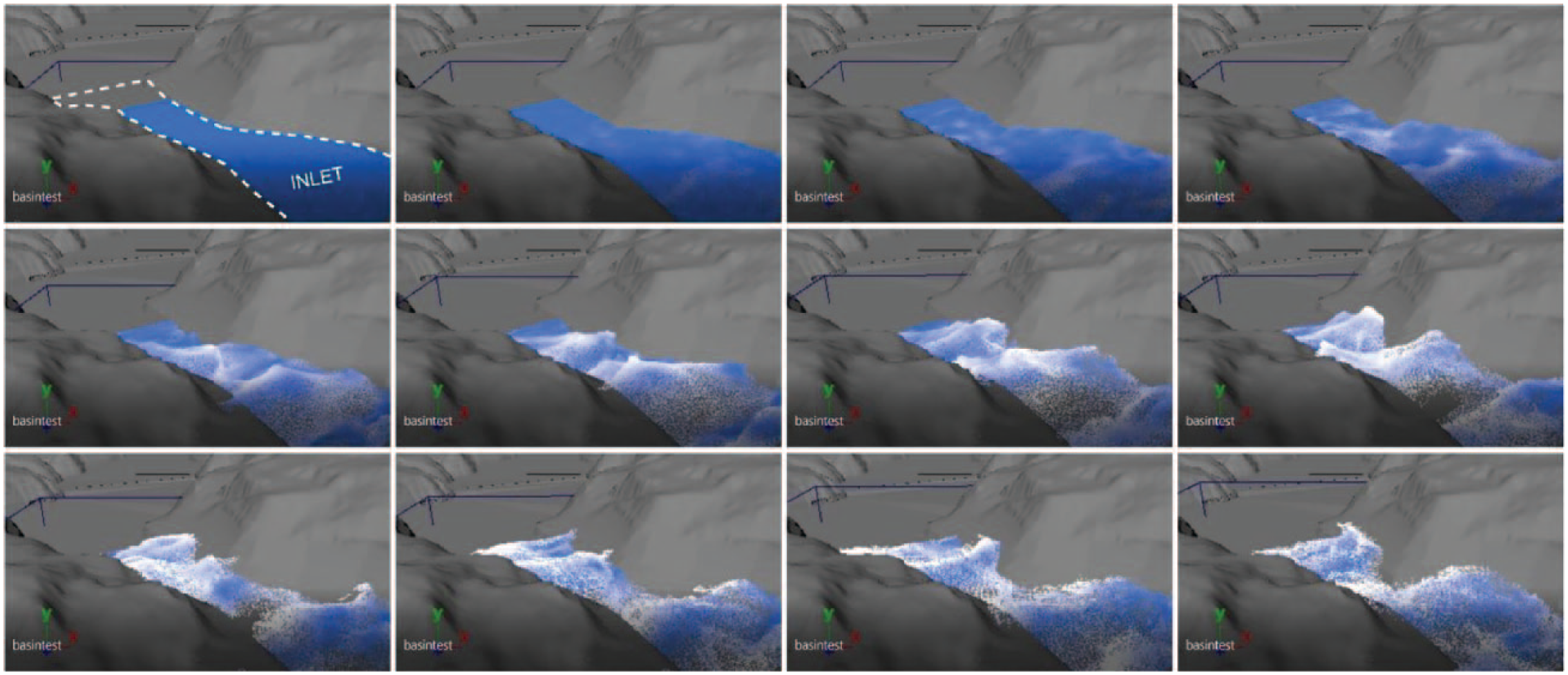
Modeling of a category 1 hurricane flowing into the re-graded inlet.
Case study 2: simulating urban heat island effects
Urban heat islands are metropolitan areas that are significantly warmer than surrounding rural areas due to human activity. The main contributing factors to urban heat islands are the presence of hardscape and concrete facades and ground materials, often comprised of darker colors which absorb and hold sunlight and increase the immediate surface temperature. This absorbed heat is then released in the cooler hours of the evening atmosphere, increasing the overall ambient temperature. The widespread use of air conditioners in densely urbanized areas are also important contributing factors, releasing heat into the atmosphere and contributing to the formation of ozone and smog. Urban temperatures can be up to 5°F–17°F warmer than surrounding suburban and rural areas, amplifying energy demand for building air conditioning, and in turn leading to greater CO2 emissions into Earth’s atmosphere. 37
With this urgency in mind, we set out to create tools and typologies to assist landscape architects, urban designers, and urban planners in mitigating urban heat island effects and reducing human reliance on artificial cooling systems during the hottest months of the year. In order to understand current conditions of urban heat island effects at a large scale, we first performed a surface temperature analysis of the entire City of Boston, MA. We used Dragonfly (a component of Ladybug Tools) to download recent data and infrared images from the USGS website and import this information to our Rhino model. To visualize, identify, and colorize the infrared image with surface temperature data, we used Ladybug to link the aerial image with aerial Landsat 38 data, where the basic infrared details were interpreted by Ladybug and Dragonfly and represented as a gradient colored by temperature range. The resulting visualization allowed us to evaluate the impact of urban heat island effects throughout the City of Boston and to identify a smaller case study area. A comparison of three neighborhoods shows varying surface temperature impacts informed by building shadow and surface material. We ultimately decided to study the Roxbury neighborhood, which included high surface temperatures as well as a higher building density than some other neighborhoods with similarly high surface temperatures (Figure 9).
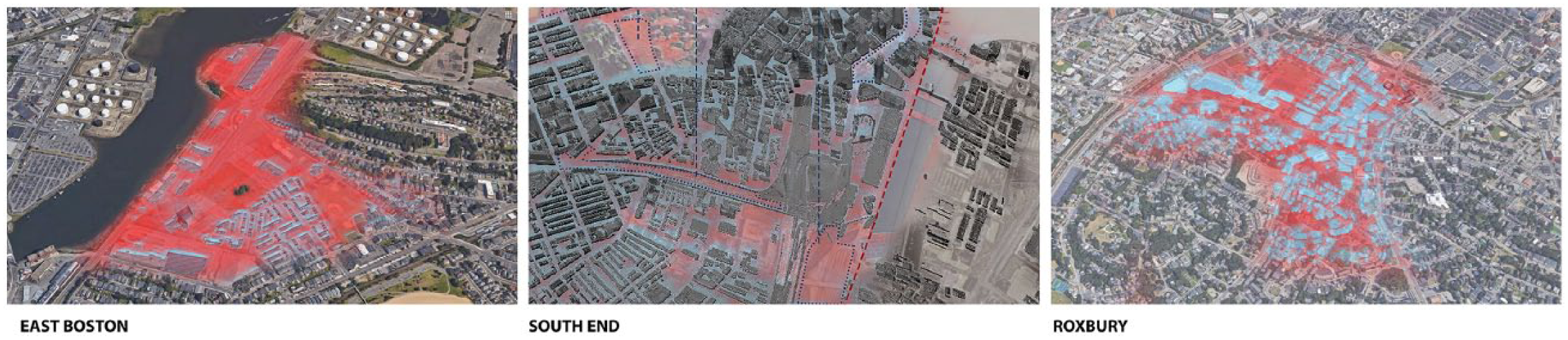
Surface temperature analysis comparison showing three neighborhoods in Boston.
Once we visualized the existing surface temperature, we proceeded with a sun and shade study. This study did not visualize the specific path of shadows cast by buildings into open space, but instead averaged the mean surface temperature which resulted from sun and shade in open areas. Each analysis was done over the course of a single month, geolocating the Rhino model to the correct geographic coordinates and orientation. Using Ladybug to identify the sun path over these set specific periods of time based on EPW data, we were able to access and apply weather data from several monitoring stations. This workflow enabled us to identify the areas of shade and sun exposure that existed across the study area within Roxbury.
These analyses showed us the major areas where surface temperature would be the hottest over the course of summer months. We identified these areas as locations where design intervention could occur to cool the surface temperature. To test design interventions which could most effectively improve these conditions, we chose two common strategies for cooling outdoor air temperature: small-scale improvements to hardscape materials and more widespread improvements to outdoor air flow. We then proceeded to use two digital workflows to test these strategies.
The first workflow of visualizing temperature differences in small-scale hardscape materials relied on computationally analyzing the impact of albedo and surface temperature. Albedo can be defined as the ability of a material to reflect solar energy. To visualize these surface temperatures based on the characteristics of their corresponding surface materials, we used the Grasshopper plugin Honeybee, a component of the Ladybug toolkit. The reliability of these tools are based on their underlying calculation of albedo, which is written here as
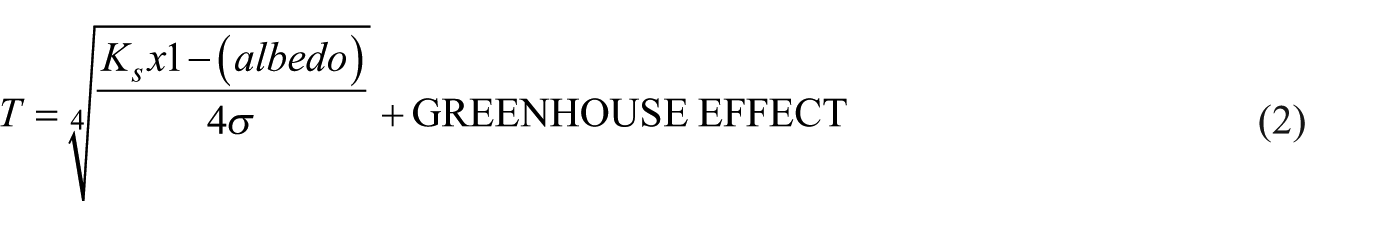
where Ks is solar insolation (“solar constant”) = 1361 Watts per square meter, σ is Stefan–Boltzmann constant = 5.670373 × 10⁻⁸ Watts/m2 K4, (m = meter, K = Kelvin), and GREENHOUSE EFFECT is 33°C.
This formula enables Honeybee to include a small number of material presets, which are embedded with data for albedo, thermal capacity, conductivity, and heat absorption. The albedo values for some of these materials are as follows:
Asphalt 0.05–0.15;
Brick 0.2–0.4;
Cement 0.7–0.8 (N);
0.2–0.3 (O);
Crushed stone 0.2–0.3;
Stone 0.2–0.4;
Wood 0.4;
Grass 0.25;
Water 0.03–0.1.
The next step was to associate ground surface textures with specific material properties, selecting and applying Honeybee presets to Rhino materials. In addition, natural elements such as trees, grass, and soil were geometrically identified to allow the Honeybee algorithm to differentiate hardscape and softscape materials. The resulting visualizations demonstrate the differences in surface temperature of the ground based on the material that was applied, indicating that soil, dry, and semi-dry sand have the highest albedo and therefore the lowest surface temperature in hot conditions (Figure 10).
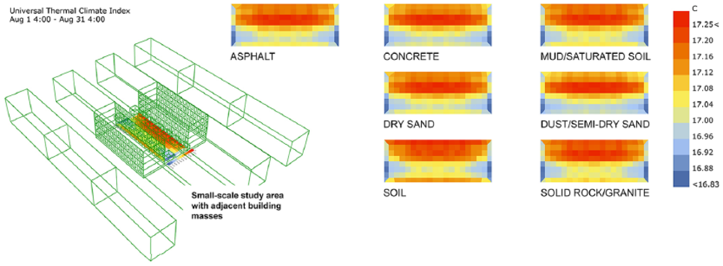
Simulation showing various materials applied to the ground plane and their resulting surface temperature.
Computationally modeling urban air flow relied on differentiating between the density, shape, and formation of buildings and the energy and seasonal direction of air flow. To understand the seasonal air flow direction, we used Ladybug to input EnergyPlus™ data to create a wind rose analysis. It is important to note that the simulations were based on current EPW data and therefore do not account for the effects of climate change on the EPW values we used. We chose this approach to avoid introducing speculative data into a new workflow which was still in a development and evaluation stage. The inclusion of well-documented methods of generating predictive EPW-based climate data will be an essential piece of our future workflows.
Once we understood the general wind direction over the course of 12 months, we selected the average hottest month of August to use as a baseline wind flow pattern for testing design strategies. Butterfly, another component of the Ladybug toolkit, relies on OpenFOAM, an open-source CFD software C++ toolbox for the development of customized numerical solvers. The CFD framework is based on the same Navier–Stokes solver as was used to create the storm surges in Bifrost and was a critical part of successfully modeling urban air flow. 20 To create this simulation, we used the Butterfly Grasshopper definition to situate the building geometries within a wind tunnel and then used the parameters within the definition to direct a series of vectors which passed across the model by way of a mesh grid. The visualization indicates the direction and speed of the vectors; as vectors were forced to change direction, slow down, or even stall, the visualization would colorize them as yellow or red. As the vectors were able to continue their path with minimal speed decrease or change in direction, they were colorized as blue. After the first simulation was complete, we adjusted the values within the Grasshopper definition, which include proposed region, wind speeds, and test period windows of time, and re-ran the simulations. The definition also provided an option to visualize air pressure, which is significant because higher air pressures lead to decreases in outdoor human comfort. The visualization shows significant portions of the study area with high surface temperature and air pressure. In the study area’s existing condition, we observed that air flow was most negatively impacted where smaller buildings were densely arranged with contrasting orientations, and we observed that air pressure was most negatively impacted where “pinch points” occurred—small areas of open space between multiple large building masses (Figure 11).
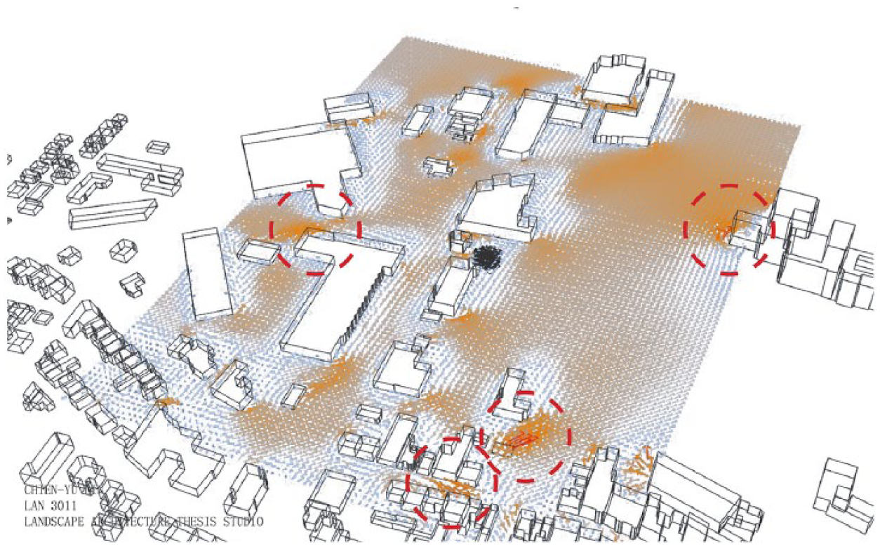
Detail of air flow simulation, showing “pinch points” between large building masses.
Once the base conditions of urban heat island effects were visualized, these same processes were used to redesign the study neighborhood as an urban design at the master plan scale. Recent research has indicated that the arrangement of a city’s streets and buildings plays a central role in how hot or cool it gets, with findings that show that a traditional urban grid, called a “crystalline” urban form, experiences more extreme heat buildup than an irregular “glass-like” formation. 39 Therefore, we decided to follow the “glass-like” formation in an attempt and redesign the neighborhood with a focus on building and street layout, coupled with simple material adjustments that would raise the overall albedo. The underlying principles of this redesign involved arranging the buildings to be as parallel to the summer wind direction as possible, with paths and roads crossing through the urban grid to channel this summer wind through open spaces.
A major advantage of using Grasshopper has been the integration of parametric tools into the visual simulation engine provided by Ladybug Tools, which played a critical role in our design decision-making. This allowed us to create variations of one environmental factor such as wind speed and visualize its impact on other environmental factors such as wind direction and air pressure (Figure 12).
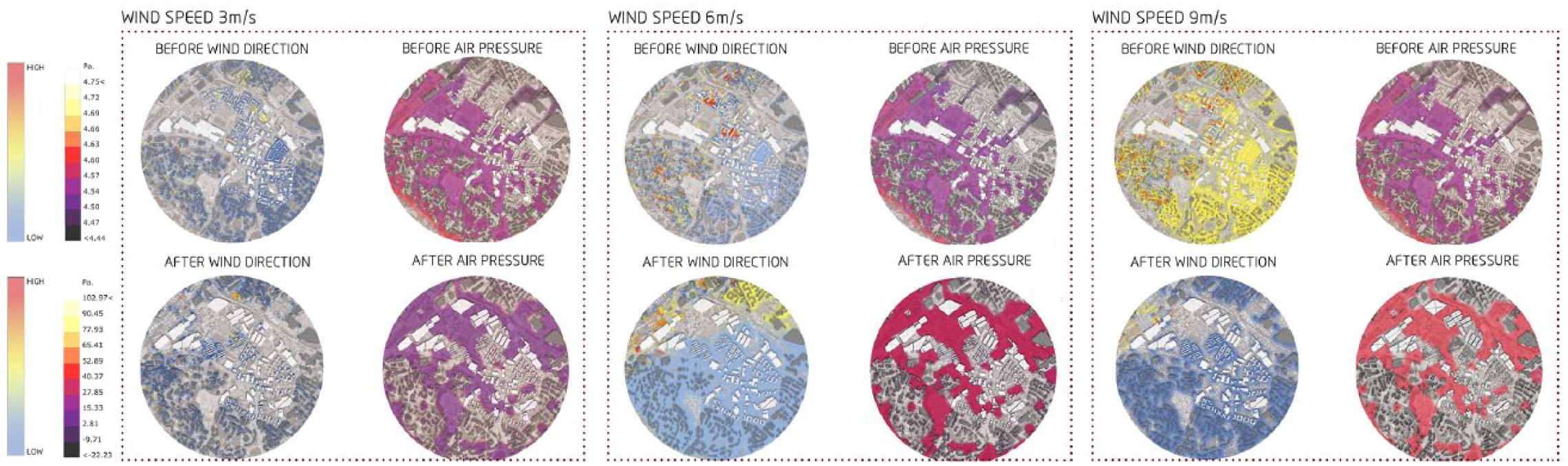
Parametric simulation of variable wind speed at 3, 6, and 9 m/s, combined with design variations and visualizing resulting effect on wind direction and air pressure.
Inserting different building and landscape formations and parametrically changing the environmental values allowed us to take advantage of the parametric capabilities of Grasshopper to confidently arrive at the most impactful design solution. Comparing the original visual simulations with simulations using the new “glass-like” urban design shows substantial improvement in the areas of surface temperature, air pressure, and air flow (Figure 13).
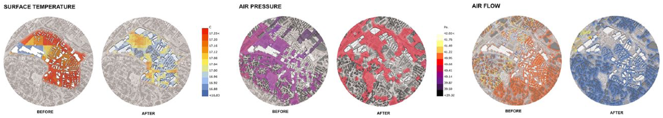
Simulations of existing conditions (left) and proposed building arrangement (right) with new hardscape materials.
Findings
The erosion simulations in this research show the increasing loss of biodiversity over time. This loss of biodiversity is clearly visible and difficult to refute in the face of the simulations we have generated. The prototype design we tested shows that coastal waters can flow inland without serious loss of property or infrastructure. This methodology helped us create quick representative models of coastal change and process that improved our understanding of the coastal systems’ complexities and irregularities, as well as the potential for landscape architecture to interrupt serious coastal damage from sea level rise and erosion. Through engaging in this process of digital modeling, the dynamism of the coastline became more observable and legible. From a biodiversity perspective, the output of these visualizations shows a future reality that has the potential to heavily disturb coastal ecology.
With regard to the erosion process, we found that there was potential to add error when retreating a coastline within Geographic Imager and Photoshop. Much of the erosion process was completed by hand, and although it was measured and methodical, we did need to make spot decisions, such as how a dune’s shape would change or remain constant. We feel comfortable with this level of personal responsibility, considering that the potential changes in future conditions of the human landscape, as well as a variety of unknowns with regard to environmental conditions, will make it difficult if not impossible to accurately model a single outcome. Rather, this research shows a range of possible conditions in order to provide a better framework for landscape architecture practice in responding to coastal change. One of the most fixed conditions is the generalized topography of the area, the major low and high elevation points. Those elevation points are the drivers for basin site selection and earthwork in this study, and therefore, we feel confident that our modeled conceptual design intervention is reasonably grounded.
The heat island simulations confirmed that alterations to surface material, building orientation and size, and scale of open spaces can dramatically improve ambient cooling of urban areas. We were surprised by the degree to which the visualizations demonstrated improved conditions and believe that they set up a strong argument for the application of these design principles in any major urban design project. Some of the simulations of surface materials proved surprising, such as the realization that wet soil is less effective at reflecting solar radiation than dry sand. Although this is logical due to material color and humidity, it is an important consideration that has emerged from this research. Especially when designing for wet conditions such as sea level rise, the use of any natural materials could seem like an entirely positive design move. The albedo simulation challenges this assumption, suggesting that some natural materials are superior to others in this regard. Another surprising finding was the “pinch points” discovery of air pressure, and its relationship to larger buildings and smaller areas of open space. Without these visualizations, we question whether reduction of air flow “pinch points” would be a primary driver of design. By visualizing these effects, we situate them at the forefront of the design process, and this initiates new thinking about spatial relationships. This may be the greatest value of these simulations: that their visual nature forces a reckoning with their principles and a greater recognition of their importance in designing for resilience.
Finally, we found that the process of engaging so many pieces of software, and the trial and error involved, could be potentially prohibitive for a deadline-driven design practice. The value of these findings might be outweighed by the cost to discover them. Through the creation of these models and simulations, we confirmed that the complexities of the natural systems we were simulating resulted in a need to assemble multiple pieces of software. These simulations required inputs from geospatial mapping, 2D image editing, 3D modeling, parametric design tools, external environmental data, and 4D animation in order to tackle a challenging, multi-scalar design dilemma. Two key concepts can be taken from this. First, applied research of this complexity might be best performed outside of any specific client project, where false starts are acceptable and to be expected. Second, there is a distinct need for a broader wraparound digital simulation solution which can accomplish more stages of these visualizations without connecting numerous pieces of software together. All told, we used five different pieces of software and three plugins to generate these discoveries. For these workflows to take hold and become normalized within professional practice, this number will need to be condensed, calling for the development of new software tools that can handle multiple pieces of these workflows under one roof.
Discussion
These two approaches address opposite ends of the climate change mitigation spectrum. One represents a long-term acceptance of sea level rise and presents a design response which works with this eventuality. The other project represents an attitude that current site-scale temperature issues can be mitigated and presents a design response which seeks to modify these issues in the short term. In the first project, the wicked problem of sea level rise has a sense of inevitability: it is on its way and is unlikely to be directly mitigated. By creating an inlet for coastal waters to reform an inland salt marsh, we argue for a responsive approach that accepts and does not fight the likelihood that coastal barrier islands will be breached within the next century. The primary goal of this design intervention was to prioritize the regeneration of coastal ecologies while reasonably preserving property and infrastructure. In contrast, the second project prioritizes human comfort through cooling. It acknowledges that site-scale landscape mitigation of heat islands can profoundly impact the ambient surface temperature in an urban area. This project suggests that designers do not need to be restricted to responsive designs when it comes to issues of outdoor thermal conditions. These issues can be directly addressed and improved through site design, with results that can be immediately perceived by humans and result in less reliance on artificial cooling systems. In turn, this can serve to reduce the overall human carbon footprint, ultimately contributing to improved long-term climate prospects. Although the current trajectory of climate change will require design adaptations which accept certain realities of sea level rise, proactive designs which reduce urban heat island effects may ultimately alter this trajectory.
Some of the preliminary efforts that went into producing these models can be reused, but they are unlikely to become automated processes. We feel that the greatest potential for automation could occur where there are reusable workflows. For example, with the coastal storm modeling in Maya, any coastal terrain mesh in the main impact area of nor’easter storms can be used with the same Bifrost simulation. This impact area includes all coastal areas between North Carolina and Massachusetts, suggesting that there is a pathway for testing this workflow on multiple sites and gathering information about its performance in differing scenarios.
The methods we used to evaluate current and future existing site conditions led directly to the generation of design solutions. In the case of the coastal storm modeling workflow, we were able to use the animated wave simulation to identify areas of ecological risk and then subsequently were able to re-run the wave simulation on an adapted terrain mesh. By subjecting the adapted terrain to the exact conditions which showed areas of risk, we were able to see specific areas where the design intervention improved or eliminated future these areas of risk. In the case of the urban heat island workflow, we were able to make specific adjustments to each of the environmental simulation parameters to identify the most problematic areas within the existing condition. As with the coastal storm workflow, we were subsequently able to re-run the urban heat island simulations with the new urban master plan. By subjecting the new master plan to the exact conditions which visualized problem areas in the existing conditions model, we were able definitively see that the problem areas had been improved. Just as importantly, we were able to ensure that no new problem areas had been created in the new master plan.
This research raises questions about the dual roles of big picture intervention and smaller, micro-scale designs, and the assumptions designers can make about what can be prevented and what is inevitable. The use of these tools for public decision-making and advocacy should be carefully considered. Greater levels of realism are suggested to encourage broader user engagement and result in a more direct communication of climate change effects but may also leave room for misinterpretation. 40 Before these types of visualizations are presented to the general public, environmental scientists should be introduced to this work and involved in further refinements. The necessary question will arise: why aren’t these scientists involved in the project from the beginning? Ultimately, this is the ideal type of interdisciplinary collaboration that will best position both designers and scientists to alter the course of climate change. However, in the near term, it may well be that scientists can provide the best feedback when they are provided an initial set of simulations with which to understand the project realities and potential design interventions. This initial presentation of graphic simulations could provide a preliminary medium for dialogue, serving as the instigator of greater engagement between designers and scientists.
Conclusion
We hope that these projects can contribute new digital workflows for architects, landscape architects, and urban designers to create resiliency in our built environment. Although computation allows designers to manage complexity and work with complex data sets, the human design eye and mind is the real tool that can interpret simulations and make decisions based on the information they provide. As we contribute more time to developing these workflows, documenting the steps we take and the discoveries they yield, we hope that they become standard practice in design environments. This methodology builds off others that are being introduced into the design profession, and owes much to the authors and anonymous contributors to these digital tools, many of which are free and open source. We hope that others will adapt the approaches we have presented and build on them to strengthen their scientific foundations and their range of visual feedback. It is imperative that all designers strive for resiliency in their work, acknowledging that every built project has an agency and can contribute to the resiliency of our built environment. These tools can inspire a designer to harness that agency.
Footnotes
Declaration of conflicting interests
The author(s) declared no potential conflicts of interest with respect to the research, authorship, and/or publication of this article.
Funding
The author(s) received no financial support for the research, authorship, and/or publication of this article.